6 Ecogeographical variables
This section names and provides description (R code with its explanation in procedure) of each of the 538 EGVs created.
Refer to the flowchart below (Fig. 6.1) for a better understanding of how these varable relate. The names used in the figure correspond to EGV layer names and follow naming convention: [group] _ [specific name] _ [scale], where:
group is a broader collection of EGVs describing the same phenomena or ecosystem, derived from the same source, etc.;
specific name briefly describes the landscape class and/or metrics used in the creation of the layer;
scale is one of: cell, 500, 1250, 3000, 10000 m around the centre of the EGV-cell. The resolution of each EGV is 1 ha; larger scales are summarised to this resolution.
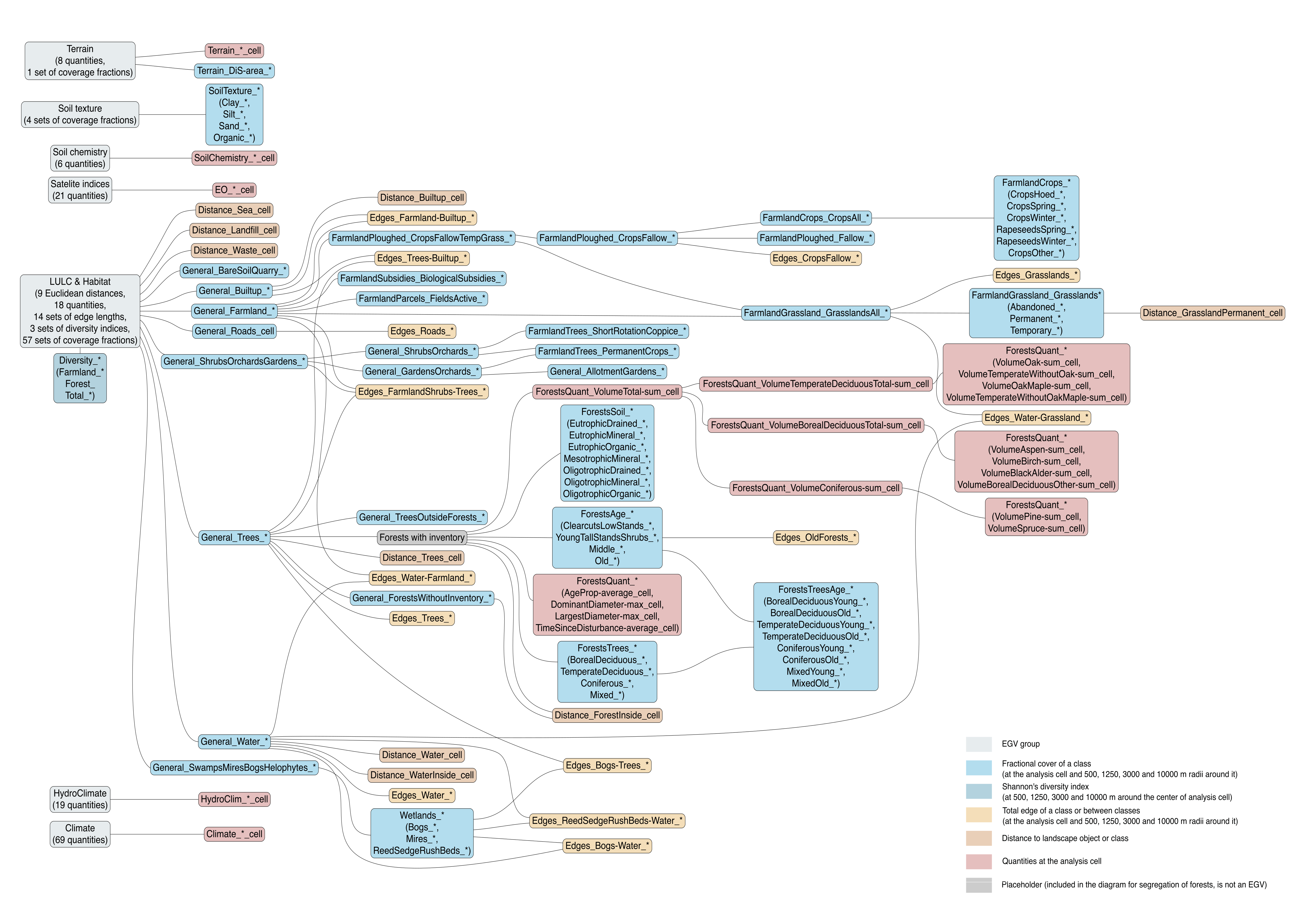
Figure 6.1: Relationships of the created ecogeographical variables.
For cover fraction and edge variables, we first calculated values at the EGV-cell
resolution and then used {exactextract} to summarise values from larger
scales. This package uses pixel area weights to calculate weighted summary
statistics, making the aggregation error negligible, particularly
at larger scales, but reduces computation time thousands up to even hundreds of
thousands times compared to input resolution (10 m). To further speed up the
procedures, we used “sparse” mode in the workflow egvtools::radius_function(), thus
summarising zonal statistics every 300 m for 3000 m radius buffers and every
1000 m for 10000 m buffers, obtaining near linear reduction in time relative to
the number of zones (ninefold and 100 fold further computation time reduction),
while loosing less than 0.001 % of variability overall.
We used a slightly different approach with diversity metrics. First, we calculated
Shanon’s diversity index at 25 ha raster grid cells, as there is nearly no
variability of landscape classes at 1 ha grid cells. Next, we calculated
arithmetic mean as zonal statictics value (using the “sparse” mode with the workflow
egvtools::radius_function()), but we did not create this EGV at the analysis
cells scale.
6.1 Climate_CHELSAv2.1-bio1_cell
filename: Climate_CHELSAv2.1-bio1_cell.tif
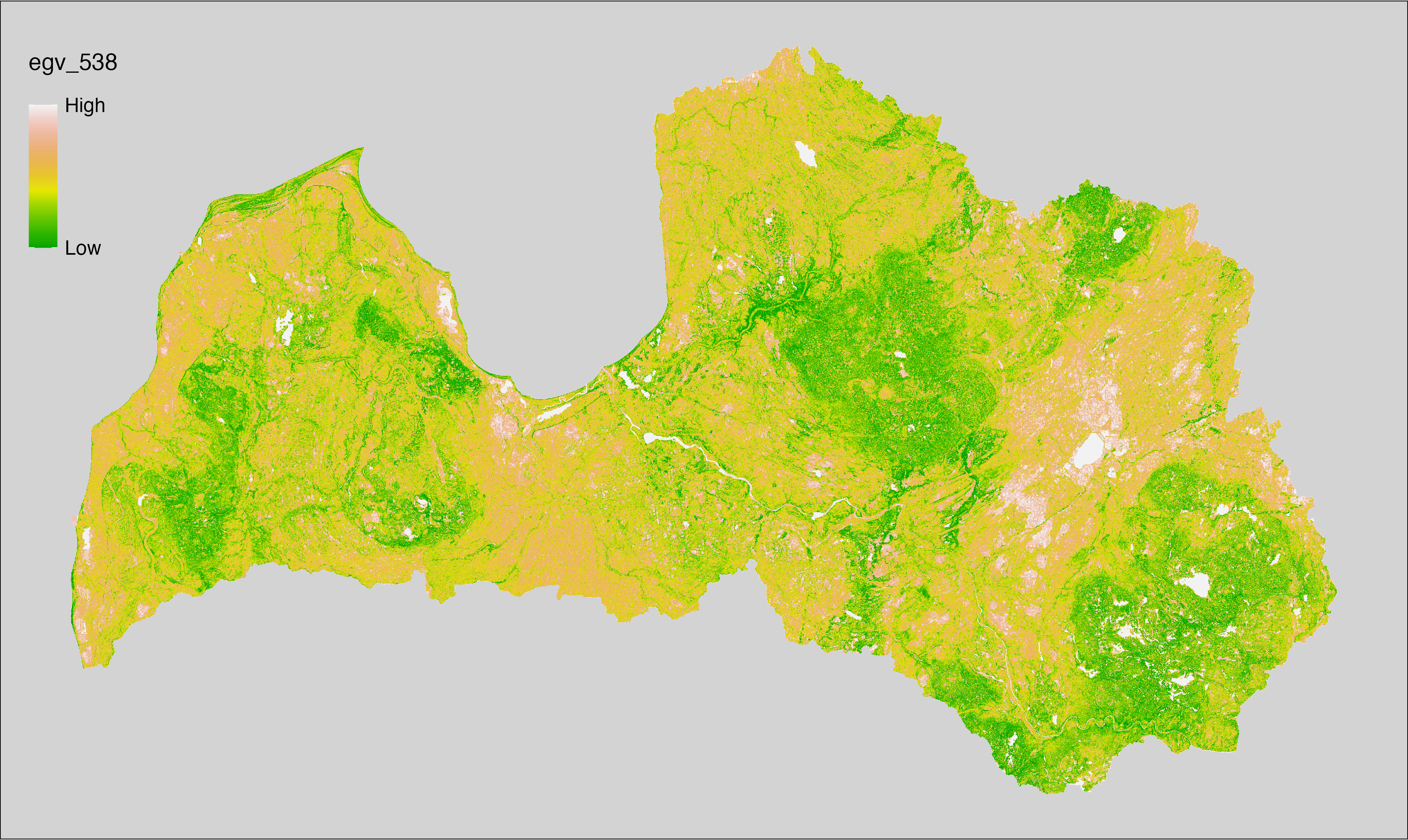
layername: egv_001
English name: Mean annual daily mean air temperature (°C) (CHELSA v2.1) within the analysis cell (1 ha)
Latvian name: Gada vidējā ik dienas vidējā gaisa temperatūra (°C) (CHELSA v2.1) analīzes šūnā (1 ha)
Procedure: Directly follows CHELSA v2.1. EGV is prepared using
the workflow egvtools::downscale2egv() with inverse distance weighted (power =
2) gap filling and soft smoothing (power = 0.5) over 5 km radius around each cell.
Finally, the layer is standardised by subtracting the arithmetic mean and
dividing by the root mean squared error.
Code
# libs ----
if(!require(egvtools)) {remotes::install_github("aavotins/egvtools"); require(egvtools)}
# job ----
localname="Climate_CHELSAv2.1-bio1_cell.tif"
layername="egv_001"
reading="./Geodata/2024/CHELSA/Climate_CHELSAv2.1-bio1_cell.tif"
df <- downscale2egv(
template_path = "./Templates/TemplateRasters/LV100m_10km.tif",
grid_path = "./Templates/TemplateGrids/tikls1km_sauzeme.parquet",
rawfile_path = reading,
out_path = "./RasterGrids_100m/2024/RAW/",
file_name = localname,
layer_name = layername,
fill_gaps = TRUE,
smooth = TRUE,
smooth_radius_km = 5,
plot_result = TRUE)
print(df)
# standardisation ----
if(!require(terra)) {install.packages("terra"); require(terra)}
if(!require(tidyverse)) {install.packages("tidyverse"); require(tidyverse)}
nosaukums="Climate_CHELSAv2.1-bio1_cell.tif"
ielasisanas_cels=paste0("./RasterGrids_100m/2024/RAW/",nosaukums)
saglabasanas_cels=paste0("./RasterGrids_100m/2024/Scaled/",nosaukums)
slanis=rast(ielasisanas_cels)
videjais=global(slanis,fun="mean",na.rm=TRUE)
centrets=slanis-videjais[,1]
standartnovirze=terra::global(centrets,fun="rms",na.rm=TRUE)
merogots=centrets/standartnovirze[,1]
writeRaster(merogots,
filename=saglabasanas_cels,
overwrite=TRUE)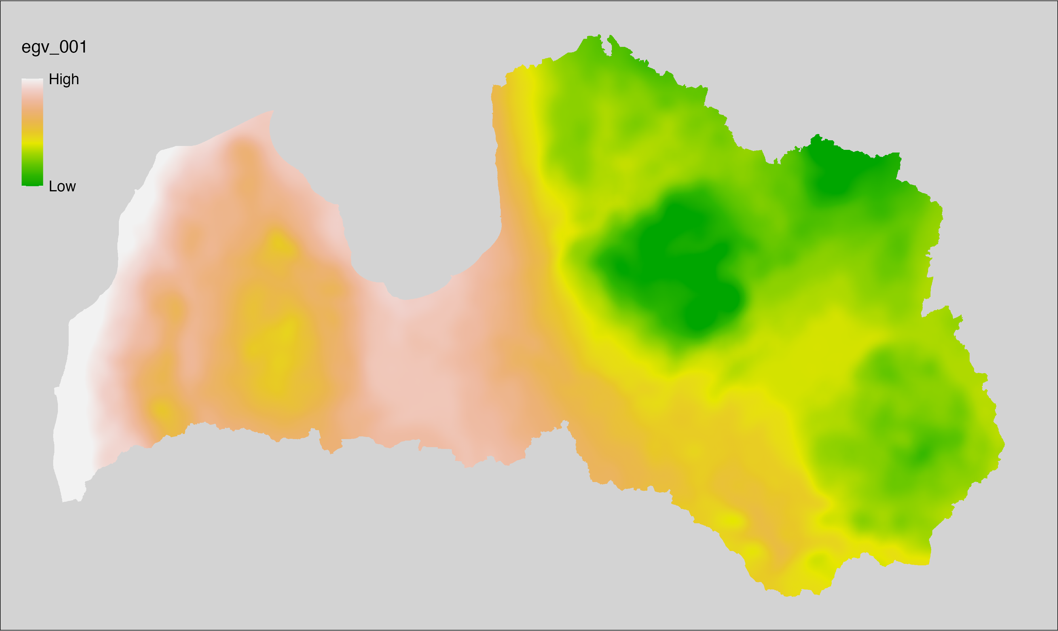
6.2 Climate_CHELSAv2.1-bio10_cell
filename: Climate_CHELSAv2.1-bio10_cell.tif
layername: egv_002
English name: Mean daily mean air temperatures (°C) of the warmest quarter (CHELSA v2.1) within the analysis cell (1 ha)
Latvian name: Gada siltākā ceturkšņa vidējā ik dienas vidējā gaisa temperatūra (°C) (CHELSA v2.1) analīzes šūnā (1 ha)
Procedure: Directly follows CHELSA v2.1. EGV is prepared using
the workflow egvtools::downscale2egv() with inverse distance weighted (power =
2) gap filling and soft smoothing (power = 0.5) over 5 km radius around each cell.
Finally, the layer is standardised by subtracting the arithmetic mean and
dividing by the root mean squared error.
Code
# libs ----
if(!require(egvtools)) {remotes::install_github("aavotins/egvtools"); require(egvtools)}
# job ----
localname="Climate_CHELSAv2.1-bio10_cell.tif"
layername="egv_002"
reading="./Geodata/2024/CHELSA/Climate_CHELSAv2.1-bio10_cell.tif"
df <- downscale2egv(
template_path = "./Templates/TemplateRasters/LV100m_10km.tif",
grid_path = "./Templates/TemplateGrids/tikls1km_sauzeme.parquet",
rawfile_path = reading,
out_path = "./RasterGrids_100m/2024/RAW/",
file_name = localname,
layer_name = layername,
fill_gaps = TRUE,
smooth = TRUE,
smooth_radius_km = 5,
plot_result = TRUE)
print(df)
# standardisation ----
if(!require(terra)) {install.packages("terra"); require(terra)}
if(!require(tidyverse)) {install.packages("tidyverse"); require(tidyverse)}
nosaukums="Climate_CHELSAv2.1-bio10_cell.tif"
ielasisanas_cels=paste0("./RasterGrids_100m/2024/RAW/",nosaukums)
saglabasanas_cels=paste0("./RasterGrids_100m/2024/Scaled/",nosaukums)
slanis=rast(ielasisanas_cels)
videjais=global(slanis,fun="mean",na.rm=TRUE)
centrets=slanis-videjais[,1]
standartnovirze=terra::global(centrets,fun="rms",na.rm=TRUE)
merogots=centrets/standartnovirze[,1]
writeRaster(merogots,
filename=saglabasanas_cels,
overwrite=TRUE)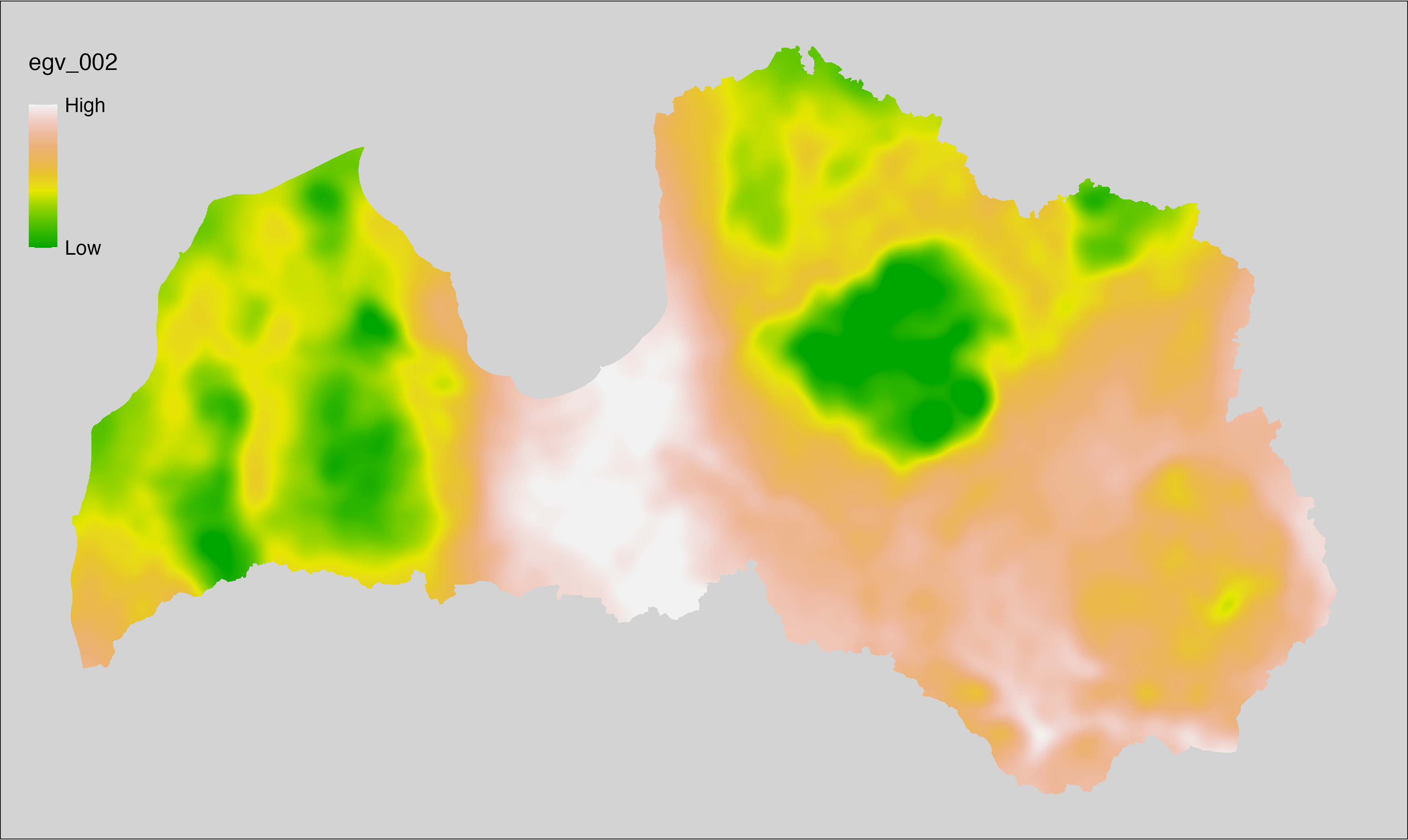
6.3 Climate_CHELSAv2.1-bio11_cell
filename: Climate_CHELSAv2.1-bio11_cell.tif
layername: egv_003
English name: Mean daily mean air temperatures (°C) of the coldest quarter (CHELSA v2.1) within the analysis cell (1 ha)
Latvian name: Gada aukstākā ceturkšņa vidējā ik dienas vidējā gaisa temperatūra (°C) (CHELSA v2.1) analīzes šūnā (1 ha)
Procedure: Directly follows CHELSA v2.1. EGV is prepared using
the workflow egvtools::downscale2egv() with inverse distance weighted (power =
2) gap filling and soft smoothing (power = 0.5) over 5 km radius around each cell.
Finally, the layer is standardised by subtracting the arithmetic mean and
dividing by the root mean squared error.
Code
# libs ----
if(!require(egvtools)) {remotes::install_github("aavotins/egvtools"); require(egvtools)}
# job ----
localname="Climate_CHELSAv2.1-bio11_cell.tif"
layername="egv_003"
reading="./Geodata/2024/CHELSA/Climate_CHELSAv2.1-bio11_cell.tif"
df <- downscale2egv(
template_path = "./Templates/TemplateRasters/LV100m_10km.tif",
grid_path = "./Templates/TemplateGrids/tikls1km_sauzeme.parquet",
rawfile_path = reading,
out_path = "./RasterGrids_100m/2024/RAW/",
file_name = localname,
layer_name = layername,
fill_gaps = TRUE,
smooth = TRUE,
smooth_radius_km = 5,
plot_result = TRUE)
print(df)
# standardisation ----
if(!require(terra)) {install.packages("terra"); require(terra)}
if(!require(tidyverse)) {install.packages("tidyverse"); require(tidyverse)}
nosaukums="Climate_CHELSAv2.1-bio11_cell.tif"
ielasisanas_cels=paste0("./RasterGrids_100m/2024/RAW/",nosaukums)
saglabasanas_cels=paste0("./RasterGrids_100m/2024/Scaled/",nosaukums)
slanis=rast(ielasisanas_cels)
videjais=global(slanis,fun="mean",na.rm=TRUE)
centrets=slanis-videjais[,1]
standartnovirze=terra::global(centrets,fun="rms",na.rm=TRUE)
merogots=centrets/standartnovirze[,1]
writeRaster(merogots,
filename=saglabasanas_cels,
overwrite=TRUE)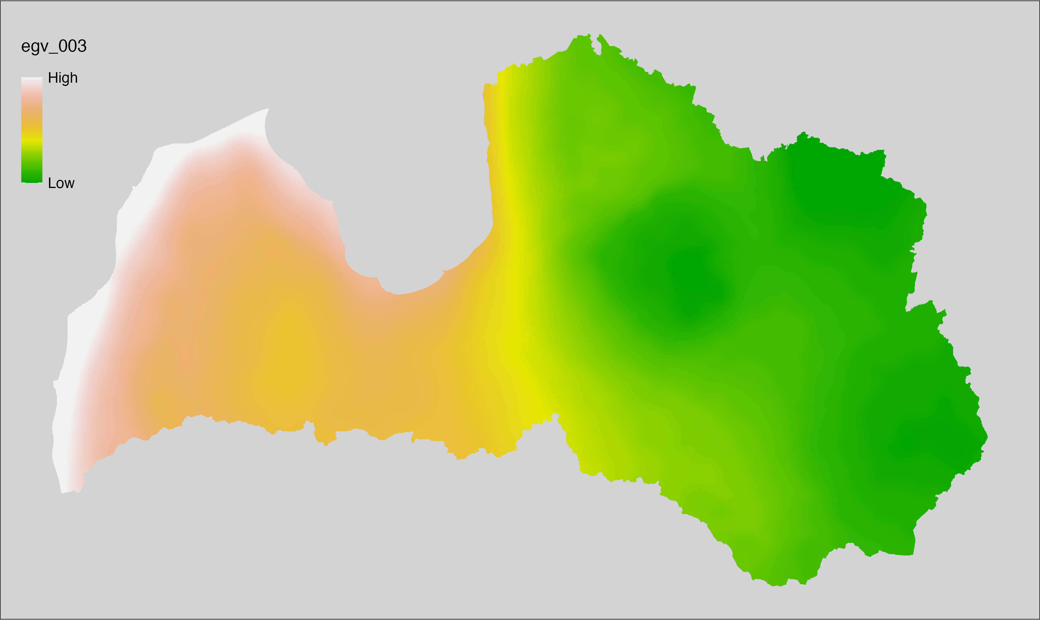
6.4 Climate_CHELSAv2.1-bio12_cell
filename: Climate_CHELSAv2.1-bio12_cell.tif
layername: egv_004
English name: Annual precipitation amount (kg m⁻² year⁻¹) (CHELSA v2.1) within the analysis cell (1 ha)
Latvian name: Nokrišņu daudzums (kg m⁻² gadā) gadā (CHELSA v2.1) analīzes šūnā (1 ha)
Procedure: Directly follows CHELSA v2.1. EGV is prepared using
the workflow egvtools::downscale2egv() with inverse distance weighted (power =
2) gap filling and soft smoothing (power = 0.5) over 5 km radius around each cell.
Finally, the layer is standardised by subtracting the arithmetic mean and
dividing by the root mean squared error.
Code
# libs ----
if(!require(egvtools)) {remotes::install_github("aavotins/egvtools"); require(egvtools)}
# job ----
localname="Climate_CHELSAv2.1-bio12_cell.tif"
layername="egv_004"
reading="./Geodata/2024/CHELSA/Climate_CHELSAv2.1-bio12_cell.tif"
df <- downscale2egv(
template_path = "./Templates/TemplateRasters/LV100m_10km.tif",
grid_path = "./Templates/TemplateGrids/tikls1km_sauzeme.parquet",
rawfile_path = reading,
out_path = "./RasterGrids_100m/2024/RAW/",
file_name = localname,
layer_name = layername,
fill_gaps = TRUE,
smooth = TRUE,
smooth_radius_km = 5,
plot_result = TRUE)
print(df)
# standardisation ----
if(!require(terra)) {install.packages("terra"); require(terra)}
if(!require(tidyverse)) {install.packages("tidyverse"); require(tidyverse)}
nosaukums="Climate_CHELSAv2.1-bio12_cell.tif"
ielasisanas_cels=paste0("./RasterGrids_100m/2024/RAW/",nosaukums)
saglabasanas_cels=paste0("./RasterGrids_100m/2024/Scaled/",nosaukums)
slanis=rast(ielasisanas_cels)
videjais=global(slanis,fun="mean",na.rm=TRUE)
centrets=slanis-videjais[,1]
standartnovirze=terra::global(centrets,fun="rms",na.rm=TRUE)
merogots=centrets/standartnovirze[,1]
writeRaster(merogots,
filename=saglabasanas_cels,
overwrite=TRUE)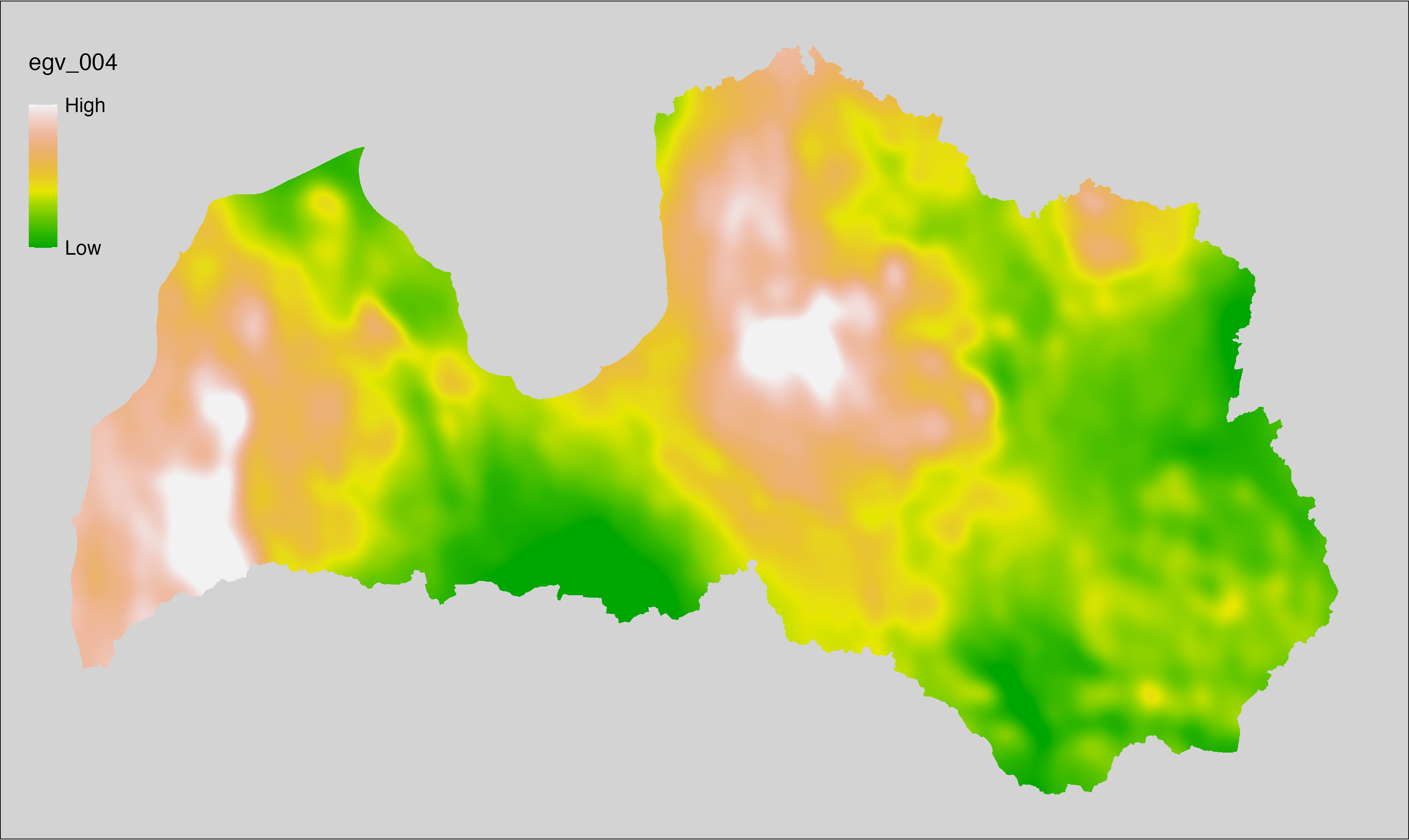
6.5 Climate_CHELSAv2.1-bio13_cell
filename: Climate_CHELSAv2.1-bio13_cell.tif
layername: egv_005
English name: Precipitation amount (kg m⁻² month⁻¹) of the wettest month (CHELSA v2.1) within the analysis cell (1 ha)
Latvian name: Slapjākā mēneša nokrišņu daudzums (kg m⁻² mēnesī) (CHELSA v2.1) analīzes šūnā (1 ha)
Procedure: Directly follows CHELSA v2.1. EGV is prepared using
the workflow egvtools::downscale2egv() with inverse distance weighted (power =
2) gap filling and soft smoothing (power = 0.5) over 5 km radius around each cell.
Finally, the layer is standardised by subtracting the arithmetic mean and
dividing by the root mean squared error.
Code
# libs ----
if(!require(egvtools)) {remotes::install_github("aavotins/egvtools"); require(egvtools)}
# job ----
localname="Climate_CHELSAv2.1-bio13_cell.tif"
layername="egv_005"
reading="./Geodata/2024/CHELSA/Climate_CHELSAv2.1-bio13_cell.tif"
df <- downscale2egv(
template_path = "./Templates/TemplateRasters/LV100m_10km.tif",
grid_path = "./Templates/TemplateGrids/tikls1km_sauzeme.parquet",
rawfile_path = reading,
out_path = "./RasterGrids_100m/2024/RAW/",
file_name = localname,
layer_name = layername,
fill_gaps = TRUE,
smooth = TRUE,
smooth_radius_km = 5,
plot_result = TRUE)
print(df)
# standardisation ----
if(!require(terra)) {install.packages("terra"); require(terra)}
if(!require(tidyverse)) {install.packages("tidyverse"); require(tidyverse)}
nosaukums="Climate_CHELSAv2.1-bio13_cell.tif"
ielasisanas_cels=paste0("./RasterGrids_100m/2024/RAW/",nosaukums)
saglabasanas_cels=paste0("./RasterGrids_100m/2024/Scaled/",nosaukums)
slanis=rast(ielasisanas_cels)
videjais=global(slanis,fun="mean",na.rm=TRUE)
centrets=slanis-videjais[,1]
standartnovirze=terra::global(centrets,fun="rms",na.rm=TRUE)
merogots=centrets/standartnovirze[,1]
writeRaster(merogots,
filename=saglabasanas_cels,
overwrite=TRUE)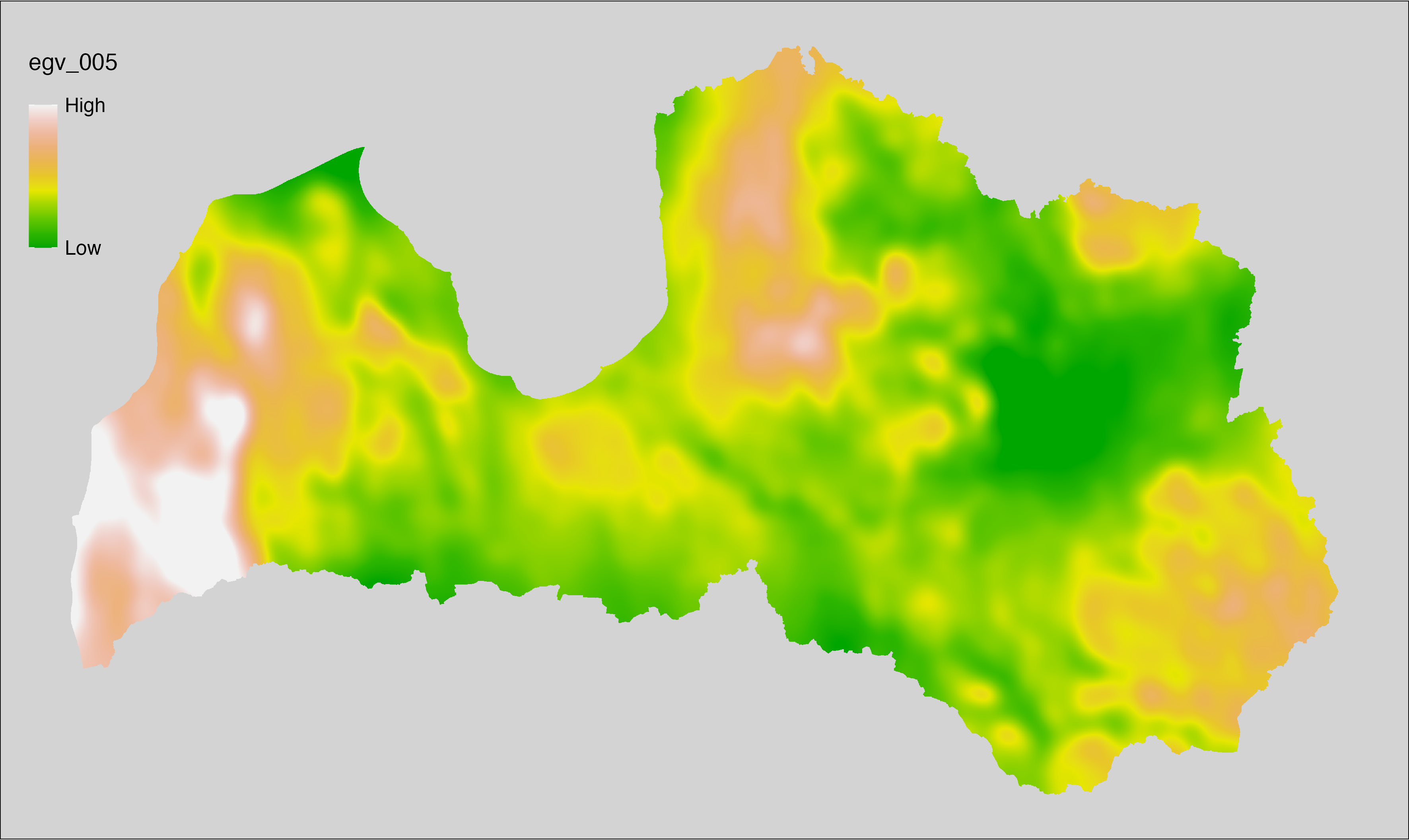
6.6 Climate_CHELSAv2.1-bio14_cell
filename: Climate_CHELSAv2.1-bio14_cell.tif
layername: egv_006
English name: Precipitation amount (kg m⁻² month⁻¹) of the driest month (CHELSA v2.1) within the analysis cell (1 ha)
Latvian name: Sausākā mēneša nokrišņu daudzums (kg m⁻² mēnesī) (CHELSA v2.1) analīzes šūnā (1 ha)
Procedure: Directly follows CHELSA v2.1. EGV is prepared using
the workflow egvtools::downscale2egv() with inverse distance weighted (power =
2) gap filling and soft smoothing (power = 0.5) over 5 km radius around each cell.
Finally, the layer is standardised by subtracting the arithmetic mean and
dividing by the root mean squared error.
Code
# libs ----
if(!require(egvtools)) {remotes::install_github("aavotins/egvtools"); require(egvtools)}
# job ----
localname="Climate_CHELSAv2.1-bio14_cell.tif"
layername="egv_006"
reading="./Geodata/2024/CHELSA/Climate_CHELSAv2.1-bio14_cell.tif"
df <- downscale2egv(
template_path = "./Templates/TemplateRasters/LV100m_10km.tif",
grid_path = "./Templates/TemplateGrids/tikls1km_sauzeme.parquet",
rawfile_path = reading,
out_path = "./RasterGrids_100m/2024/RAW/",
file_name = localname,
layer_name = layername,
fill_gaps = TRUE,
smooth = TRUE,
smooth_radius_km = 5,
plot_result = TRUE)
print(df)
# standardisation ----
if(!require(terra)) {install.packages("terra"); require(terra)}
if(!require(tidyverse)) {install.packages("tidyverse"); require(tidyverse)}
nosaukums="Climate_CHELSAv2.1-bio14_cell.tif"
ielasisanas_cels=paste0("./RasterGrids_100m/2024/RAW/",nosaukums)
saglabasanas_cels=paste0("./RasterGrids_100m/2024/Scaled/",nosaukums)
slanis=rast(ielasisanas_cels)
videjais=global(slanis,fun="mean",na.rm=TRUE)
centrets=slanis-videjais[,1]
standartnovirze=terra::global(centrets,fun="rms",na.rm=TRUE)
merogots=centrets/standartnovirze[,1]
writeRaster(merogots,
filename=saglabasanas_cels,
overwrite=TRUE)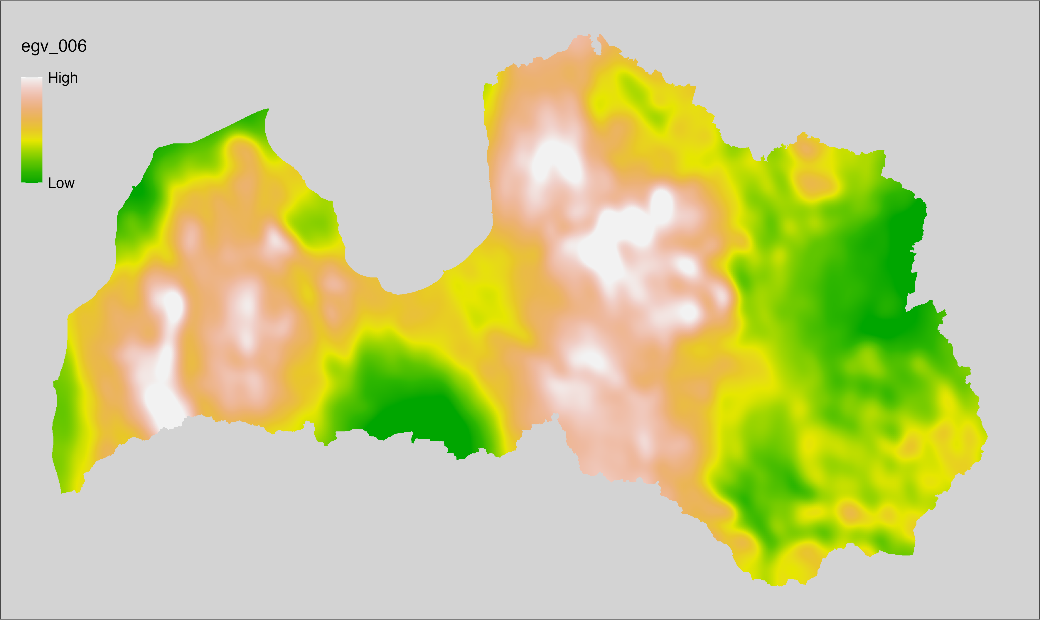
6.7 Climate_CHELSAv2.1-bio15_cell
filename: Climate_CHELSAv2.1-bio15_cell.tif
layername: egv_007
English name: Precipitation seasonality (kg m⁻²) (CHELSA v2.1) within the analysis cell (1 ha)
Latvian name: Nokrišņu sezonalitāte (kg m⁻²) (CHELSA v2.1) analīzes šūnā (1 ha)
Procedure: Directly follows CHELSA v2.1. EGV is prepared using
the workflow egvtools::downscale2egv() with inverse distance weighted (power =
2) gap filling and soft smoothing (power = 0.5) over 5 km radius around each cell.
Finally, the layer is standardised by subtracting the arithmetic mean and
dividing by the root mean squared error.
Code
# libs ----
if(!require(egvtools)) {remotes::install_github("aavotins/egvtools"); require(egvtools)}
# job ----
localname="Climate_CHELSAv2.1-bio15_cell.tif"
layername="egv_007"
reading="./Geodata/2024/CHELSA/Climate_CHELSAv2.1-bio15_cell.tif"
df <- downscale2egv(
template_path = "./Templates/TemplateRasters/LV100m_10km.tif",
grid_path = "./Templates/TemplateGrids/tikls1km_sauzeme.parquet",
rawfile_path = reading,
out_path = "./RasterGrids_100m/2024/RAW/",
file_name = localname,
layer_name = layername,
fill_gaps = TRUE,
smooth = TRUE,
smooth_radius_km = 5,
plot_result = TRUE)
print(df)
# standardisation ----
if(!require(terra)) {install.packages("terra"); require(terra)}
if(!require(tidyverse)) {install.packages("tidyverse"); require(tidyverse)}
nosaukums="Climate_CHELSAv2.1-bio15_cell.tif"
ielasisanas_cels=paste0("./RasterGrids_100m/2024/RAW/",nosaukums)
saglabasanas_cels=paste0("./RasterGrids_100m/2024/Scaled/",nosaukums)
slanis=rast(ielasisanas_cels)
videjais=global(slanis,fun="mean",na.rm=TRUE)
centrets=slanis-videjais[,1]
standartnovirze=terra::global(centrets,fun="rms",na.rm=TRUE)
merogots=centrets/standartnovirze[,1]
writeRaster(merogots,
filename=saglabasanas_cels,
overwrite=TRUE)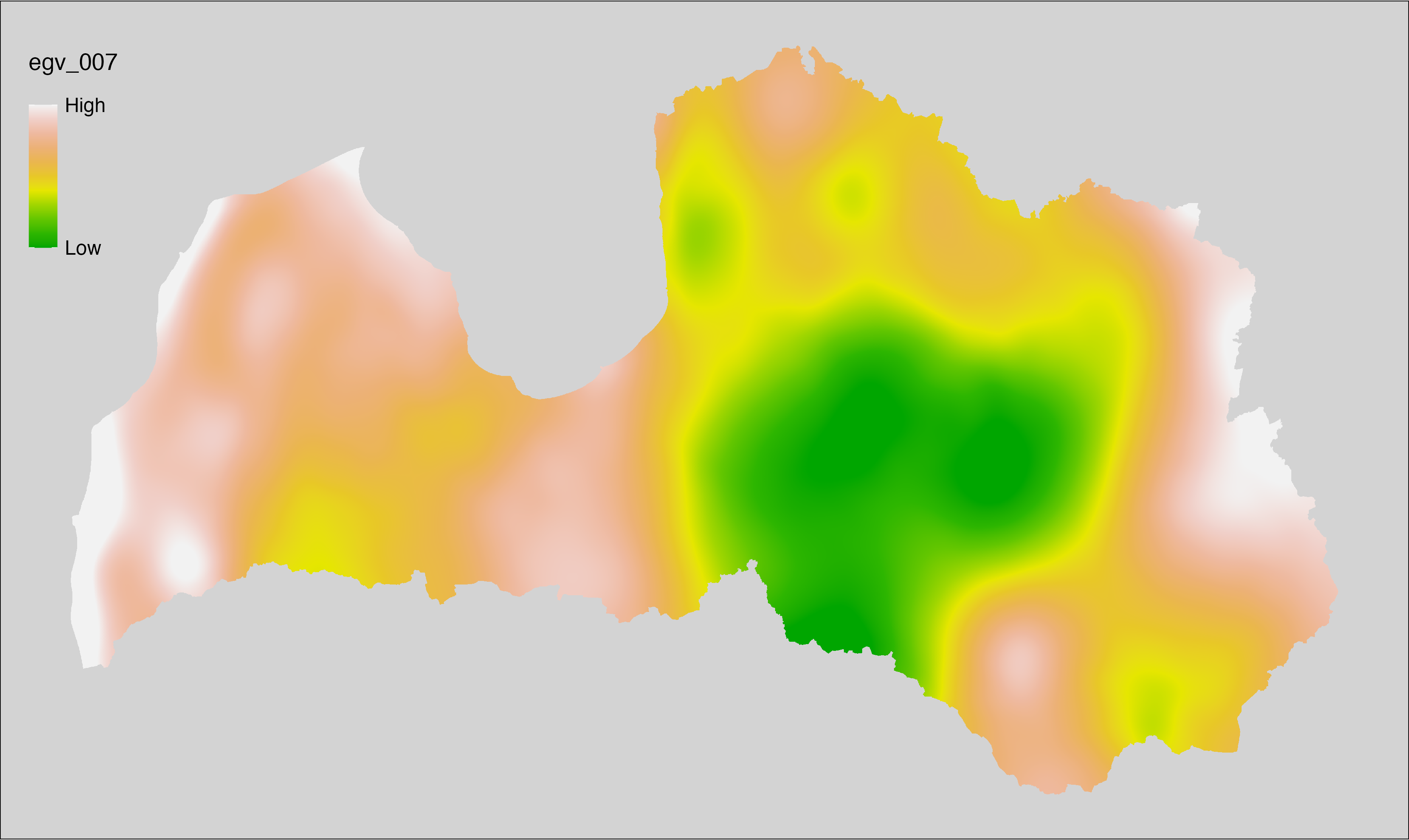
6.8 Climate_CHELSAv2.1-bio16_cell
filename: Climate_CHELSAv2.1-bio16_cell.tif
layername: egv_008
English name: Mean monthly precipitation amount (kg m⁻² month⁻¹) of the wettest quarter (CHELSA v2.1) within the analysis cell (1 ha)
Latvian name: Slapjākā ceturkšņa vidējais nokrišņu daudzums mēnesī (kg m⁻² mēnesī) (CHELSA v2.1) analīzes šūnā (1 ha)
Procedure: Directly follows CHELSA v2.1. EGV is prepared using
the workflow egvtools::downscale2egv() with inverse distance weighted (power =
2) gap filling and soft smoothing (power = 0.5) over 5 km radius around each cell.
Finally, the layer is standardised by subtracting the arithmetic mean and
dividing by the root mean squared error.
Code
# libs ----
if(!require(egvtools)) {remotes::install_github("aavotins/egvtools"); require(egvtools)}
# job ----
localname="Climate_CHELSAv2.1-bio16_cell.tif"
layername="egv_008"
reading="./Geodata/2024/CHELSA/Climate_CHELSAv2.1-bio16_cell.tif"
df <- downscale2egv(
template_path = "./Templates/TemplateRasters/LV100m_10km.tif",
grid_path = "./Templates/TemplateGrids/tikls1km_sauzeme.parquet",
rawfile_path = reading,
out_path = "./RasterGrids_100m/2024/RAW/",
file_name = localname,
layer_name = layername,
fill_gaps = TRUE,
smooth = TRUE,
smooth_radius_km = 5,
plot_result = TRUE)
print(df)
# standardisation ----
if(!require(terra)) {install.packages("terra"); require(terra)}
if(!require(tidyverse)) {install.packages("tidyverse"); require(tidyverse)}
nosaukums="Climate_CHELSAv2.1-bio16_cell.tif"
ielasisanas_cels=paste0("./RasterGrids_100m/2024/RAW/",nosaukums)
saglabasanas_cels=paste0("./RasterGrids_100m/2024/Scaled/",nosaukums)
slanis=rast(ielasisanas_cels)
videjais=global(slanis,fun="mean",na.rm=TRUE)
centrets=slanis-videjais[,1]
standartnovirze=terra::global(centrets,fun="rms",na.rm=TRUE)
merogots=centrets/standartnovirze[,1]
writeRaster(merogots,
filename=saglabasanas_cels,
overwrite=TRUE)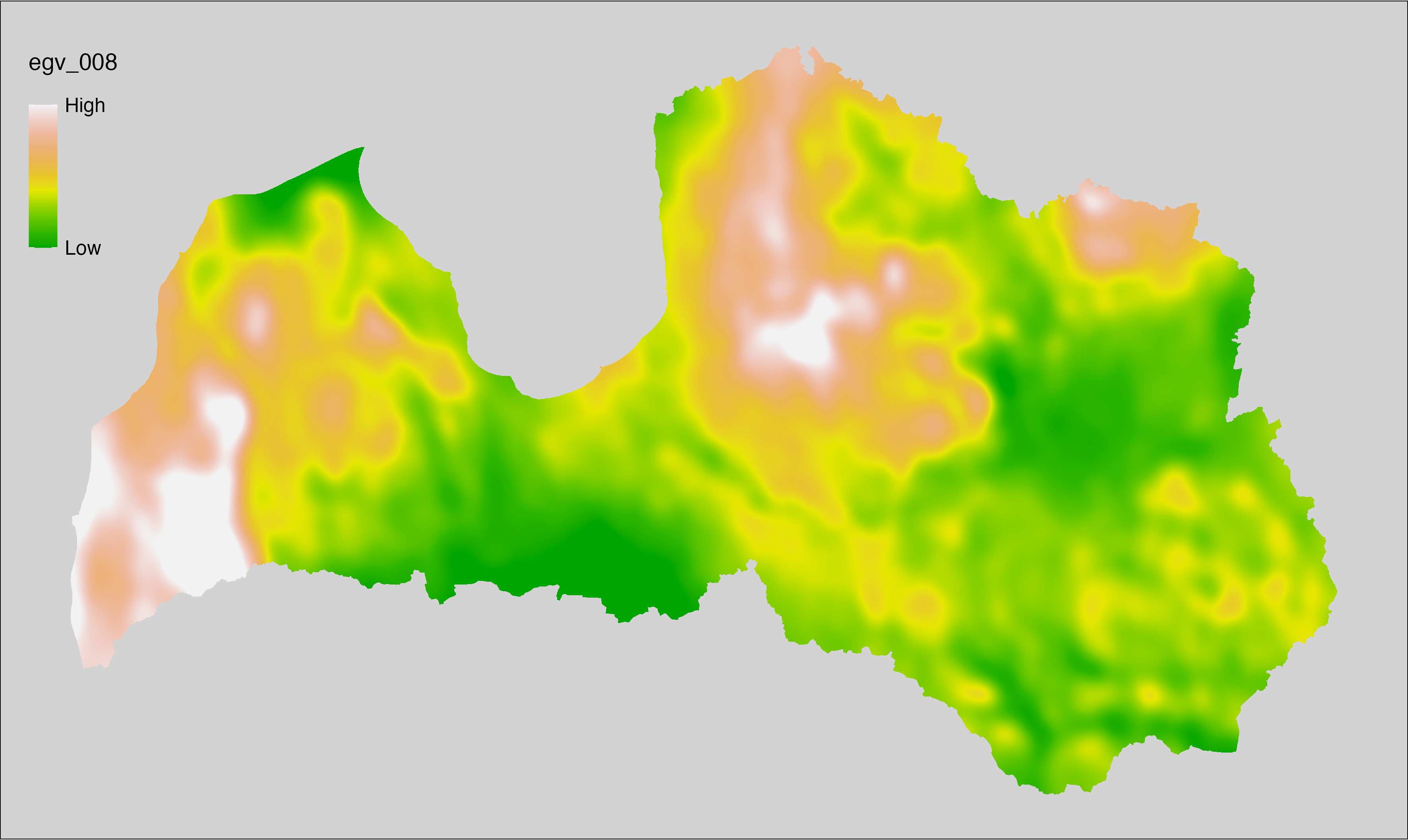
6.9 Climate_CHELSAv2.1-bio17_cell
filename: Climate_CHELSAv2.1-bio17_cell.tif
layername: egv_009
English name: Mean monthly precipitation amount (kg m⁻² month⁻¹) of the driest quarter (CHELSA v2.1) within the analysis cell (1 ha)
Latvian name: Sausākā ceturkšņa vidējais nokrišņu daudzums mēnesī (kg m⁻² mēnesī) (CHELSA v2.1) analīzes šūnā (1 ha)
Procedure: Directly follows CHELSA v2.1. EGV is prepared using
the workflow egvtools::downscale2egv() with inverse distance weighted (power =
2) gap filling and soft smoothing (power = 0.5) over 5 km radius around each cell.
Finally, the layer is standardised by subtracting the arithmetic mean and
dividing by the root mean squared error.
Code
# libs ----
if(!require(egvtools)) {remotes::install_github("aavotins/egvtools"); require(egvtools)}
# job ----
localname="Climate_CHELSAv2.1-bio17_cell.tif"
layername="egv_009"
reading="./Geodata/2024/CHELSA/Climate_CHELSAv2.1-bio17_cell.tif"
df <- downscale2egv(
template_path = "./Templates/TemplateRasters/LV100m_10km.tif",
grid_path = "./Templates/TemplateGrids/tikls1km_sauzeme.parquet",
rawfile_path = reading,
out_path = "./RasterGrids_100m/2024/RAW/",
file_name = localname,
layer_name = layername,
fill_gaps = TRUE,
smooth = TRUE,
smooth_radius_km = 5,
plot_result = TRUE)
print(df)
# standardisation ----
if(!require(terra)) {install.packages("terra"); require(terra)}
if(!require(tidyverse)) {install.packages("tidyverse"); require(tidyverse)}
nosaukums="Climate_CHELSAv2.1-bio17_cell.tif"
ielasisanas_cels=paste0("./RasterGrids_100m/2024/RAW/",nosaukums)
saglabasanas_cels=paste0("./RasterGrids_100m/2024/Scaled/",nosaukums)
slanis=rast(ielasisanas_cels)
videjais=global(slanis,fun="mean",na.rm=TRUE)
centrets=slanis-videjais[,1]
standartnovirze=terra::global(centrets,fun="rms",na.rm=TRUE)
merogots=centrets/standartnovirze[,1]
writeRaster(merogots,
filename=saglabasanas_cels,
overwrite=TRUE)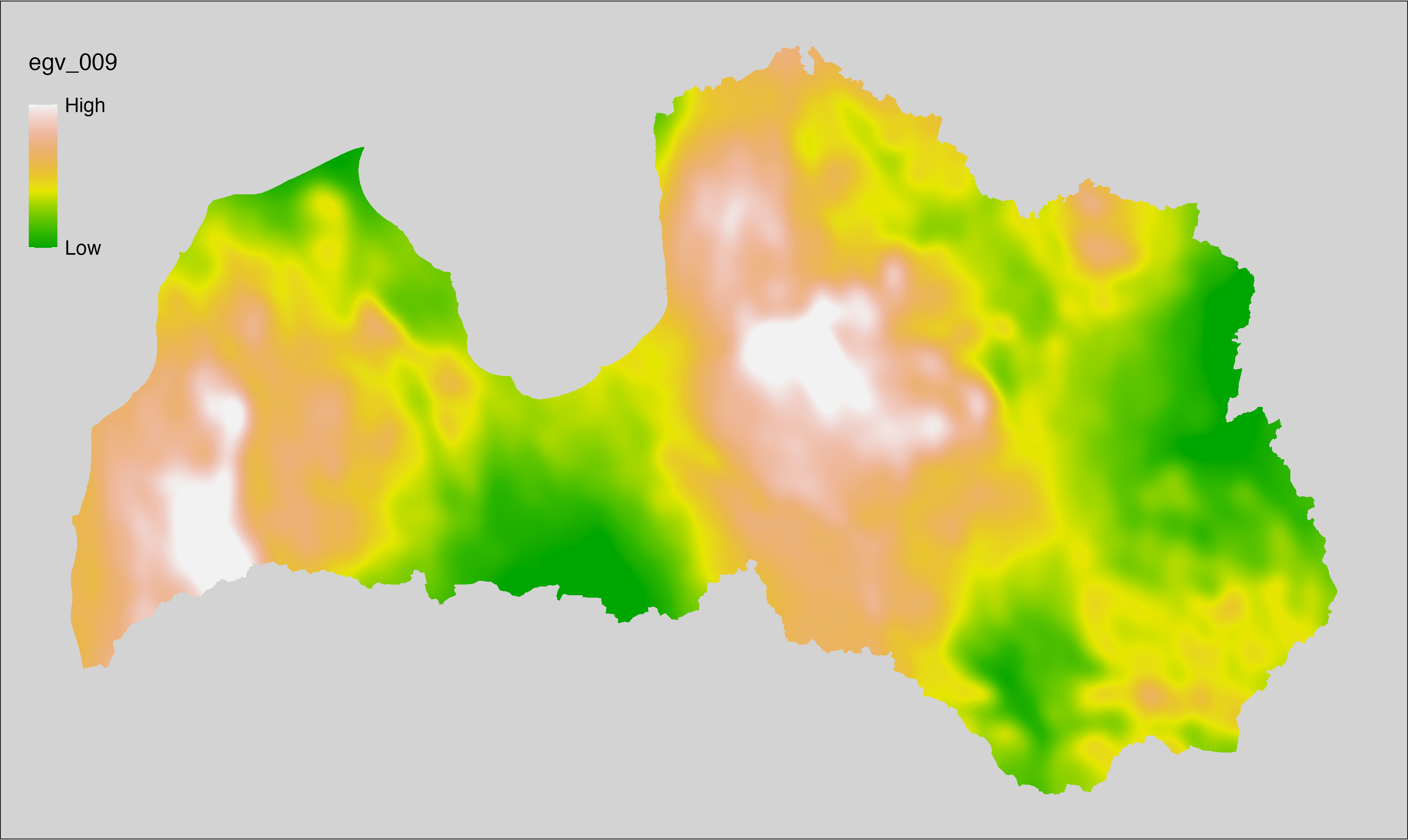
6.10 Climate_CHELSAv2.1-bio18_cell
filename: Climate_CHELSAv2.1-bio18_cell.tif
layername: egv_010
English name: Mean monthly precipitation amount (kg m⁻² month⁻¹) of the warmest quarter (CHELSA v2.1) within the analysis cell (1 ha)
Latvian name: Siltākā ceturkšņa vidējais nokrišņu daudzums mēnesī (kg m⁻² mēnesī) (CHELSA v2.1) analīzes šūnā (1 ha)
Procedure: Directly follows CHELSA v2.1. EGV is prepared using
the workflow egvtools::downscale2egv() with inverse distance weighted (power =
2) gap filling and soft smoothing (power = 0.5) over 5 km radius around each cell.
Finally, the layer is standardised by subtracting the arithmetic mean and
dividing by the root mean squared error.
Code
# libs ----
if(!require(egvtools)) {remotes::install_github("aavotins/egvtools"); require(egvtools)}
# job ----
localname="Climate_CHELSAv2.1-bio18_cell.tif"
layername="egv_010"
reading="./Geodata/2024/CHELSA/Climate_CHELSAv2.1-bio18_cell.tif"
df <- downscale2egv(
template_path = "./Templates/TemplateRasters/LV100m_10km.tif",
grid_path = "./Templates/TemplateGrids/tikls1km_sauzeme.parquet",
rawfile_path = reading,
out_path = "./RasterGrids_100m/2024/RAW/",
file_name = localname,
layer_name = layername,
fill_gaps = TRUE,
smooth = TRUE,
smooth_radius_km = 5,
plot_result = TRUE)
print(df)
# standardisation ----
if(!require(terra)) {install.packages("terra"); require(terra)}
if(!require(tidyverse)) {install.packages("tidyverse"); require(tidyverse)}
nosaukums="Climate_CHELSAv2.1-bio18_cell.tif"
ielasisanas_cels=paste0("./RasterGrids_100m/2024/RAW/",nosaukums)
saglabasanas_cels=paste0("./RasterGrids_100m/2024/Scaled/",nosaukums)
slanis=rast(ielasisanas_cels)
videjais=global(slanis,fun="mean",na.rm=TRUE)
centrets=slanis-videjais[,1]
standartnovirze=terra::global(centrets,fun="rms",na.rm=TRUE)
merogots=centrets/standartnovirze[,1]
writeRaster(merogots,
filename=saglabasanas_cels,
overwrite=TRUE)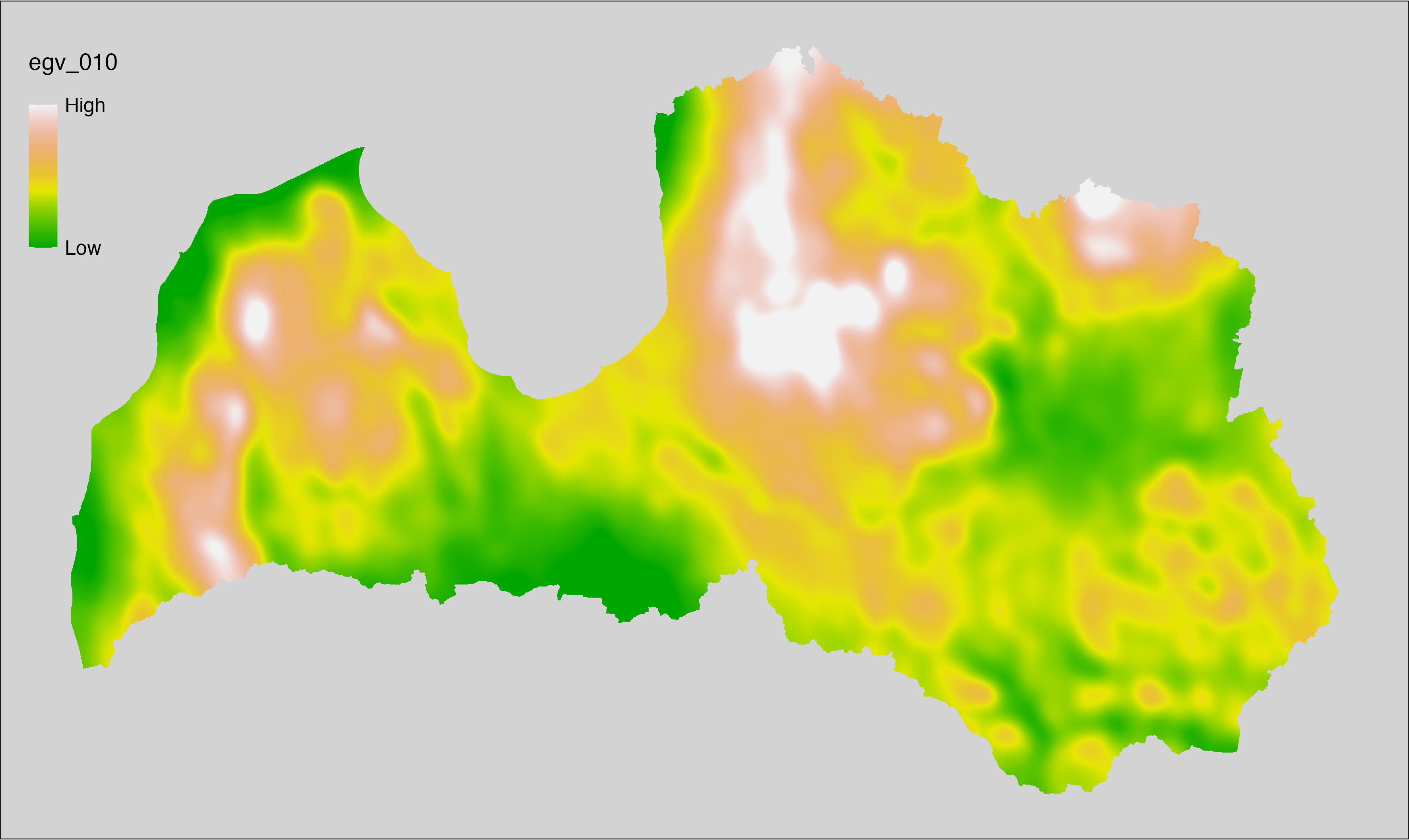
6.11 Climate_CHELSAv2.1-bio19_cell
filename: Climate_CHELSAv2.1-bio19_cell.tif
layername: egv_011
English name: Mean monthly precipitation amount (kg m⁻² month⁻¹) of the coldest quarter (CHELSA v2.1) within the analysis cell (1 ha)
Latvian name: Aukstākā ceturkšņa vidējais nokrišņu daudzums mēnesī (kg m⁻² mēnesī) (CHELSA v2.1) analīzes šūnā (1 ha)
Procedure: Directly follows CHELSA v2.1. EGV is prepared using
the workflow egvtools::downscale2egv() with inverse distance weighted (power =
2) gap filling and soft smoothing (power = 0.5) over 5 km radius around each cell.
Finally, the layer is standardised by subtracting the arithmetic mean and
dividing by the root mean squared error.
Code
# libs ----
if(!require(egvtools)) {remotes::install_github("aavotins/egvtools"); require(egvtools)}
# job ----
localname="Climate_CHELSAv2.1-bio19_cell.tif"
layername="egv_011"
reading="./Geodata/2024/CHELSA/Climate_CHELSAv2.1-bio19_cell.tif"
df <- downscale2egv(
template_path = "./Templates/TemplateRasters/LV100m_10km.tif",
grid_path = "./Templates/TemplateGrids/tikls1km_sauzeme.parquet",
rawfile_path = reading,
out_path = "./RasterGrids_100m/2024/RAW/",
file_name = localname,
layer_name = layername,
fill_gaps = TRUE,
smooth = TRUE,
smooth_radius_km = 5,
plot_result = TRUE)
print(df)
# standardisation ----
if(!require(terra)) {install.packages("terra"); require(terra)}
if(!require(tidyverse)) {install.packages("tidyverse"); require(tidyverse)}
nosaukums="Climate_CHELSAv2.1-bio19_cell.tif"
ielasisanas_cels=paste0("./RasterGrids_100m/2024/RAW/",nosaukums)
saglabasanas_cels=paste0("./RasterGrids_100m/2024/Scaled/",nosaukums)
slanis=rast(ielasisanas_cels)
videjais=global(slanis,fun="mean",na.rm=TRUE)
centrets=slanis-videjais[,1]
standartnovirze=terra::global(centrets,fun="rms",na.rm=TRUE)
merogots=centrets/standartnovirze[,1]
writeRaster(merogots,
filename=saglabasanas_cels,
overwrite=TRUE)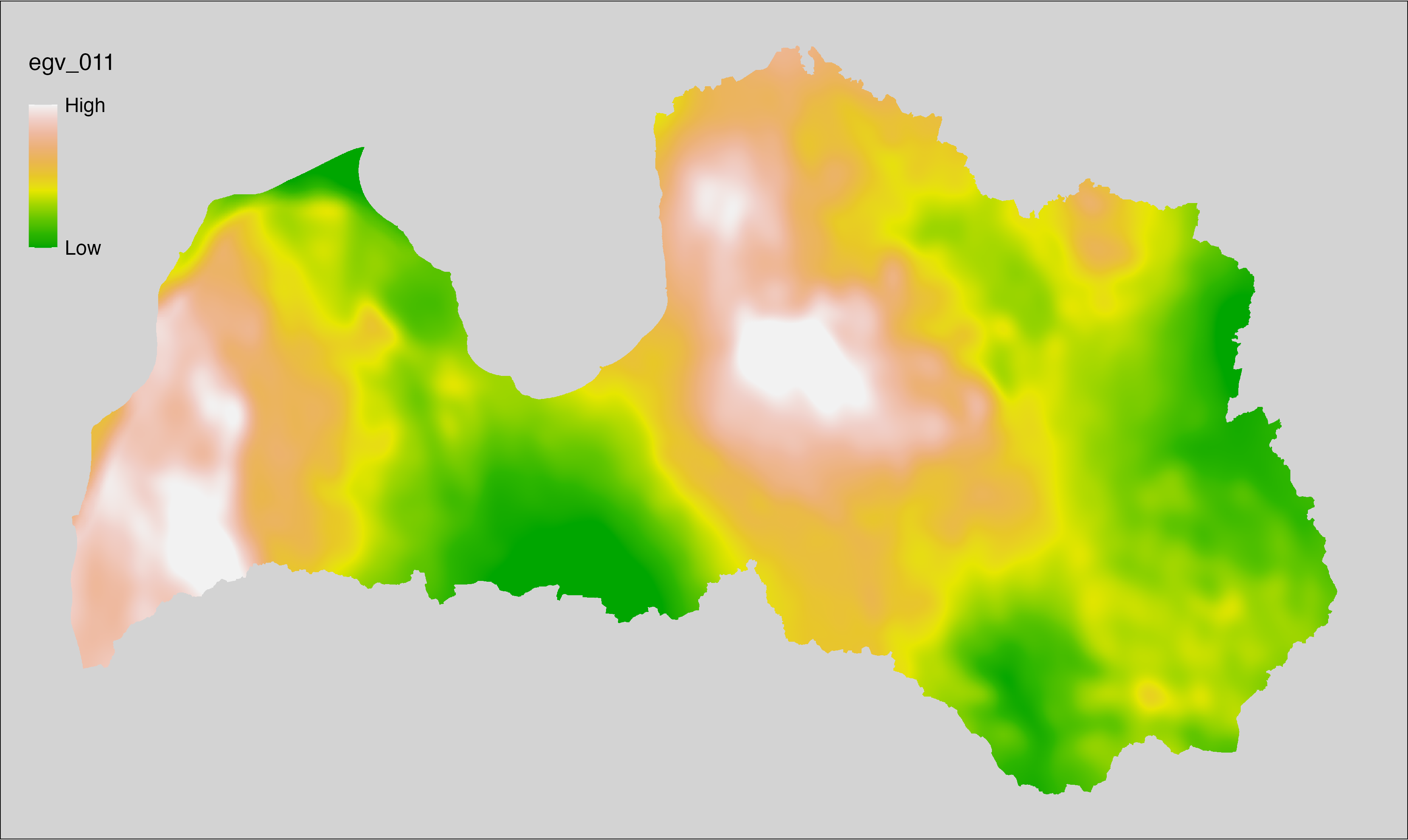
6.12 Climate_CHELSAv2.1-bio2_cell
filename: Climate_CHELSAv2.1-bio2_cell.tif
layername: egv_012
English name: Mean diurnal air temperature range (°C) (CHELSA v2.1) within the analysis cell (1 ha)
Latvian name: Vidējā diennakts gaisa temperatūru amplitūda (°C) (CHELSA v2.1) analīzes šūnā (1 ha)
Procedure: Directly follows CHELSA v2.1. EGV is prepared using
the workflow egvtools::downscale2egv() with inverse distance weighted (power =
2) gap filling and soft smoothing (power = 0.5) over 5 km radius around each cell.
Finally, the layer is standardised by subtracting the arithmetic mean and
dividing by the root mean squared error.
Code
# libs ----
if(!require(egvtools)) {remotes::install_github("aavotins/egvtools"); require(egvtools)}
# job ----
localname="Climate_CHELSAv2.1-bio2_cell.tif"
layername="egv_012"
reading="./Geodata/2024/CHELSA/Climate_CHELSAv2.1-bio2_cell.tif"
df <- downscale2egv(
template_path = "./Templates/TemplateRasters/LV100m_10km.tif",
grid_path = "./Templates/TemplateGrids/tikls1km_sauzeme.parquet",
rawfile_path = reading,
out_path = "./RasterGrids_100m/2024/RAW/",
file_name = localname,
layer_name = layername,
fill_gaps = TRUE,
smooth = TRUE,
smooth_radius_km = 5,
plot_result = TRUE)
print(df)
# standardisation ----
if(!require(terra)) {install.packages("terra"); require(terra)}
if(!require(tidyverse)) {install.packages("tidyverse"); require(tidyverse)}
nosaukums="Climate_CHELSAv2.1-bio2_cell.tif"
ielasisanas_cels=paste0("./RasterGrids_100m/2024/RAW/",nosaukums)
saglabasanas_cels=paste0("./RasterGrids_100m/2024/Scaled/",nosaukums)
slanis=rast(ielasisanas_cels)
videjais=global(slanis,fun="mean",na.rm=TRUE)
centrets=slanis-videjais[,1]
standartnovirze=terra::global(centrets,fun="rms",na.rm=TRUE)
merogots=centrets/standartnovirze[,1]
writeRaster(merogots,
filename=saglabasanas_cels,
overwrite=TRUE)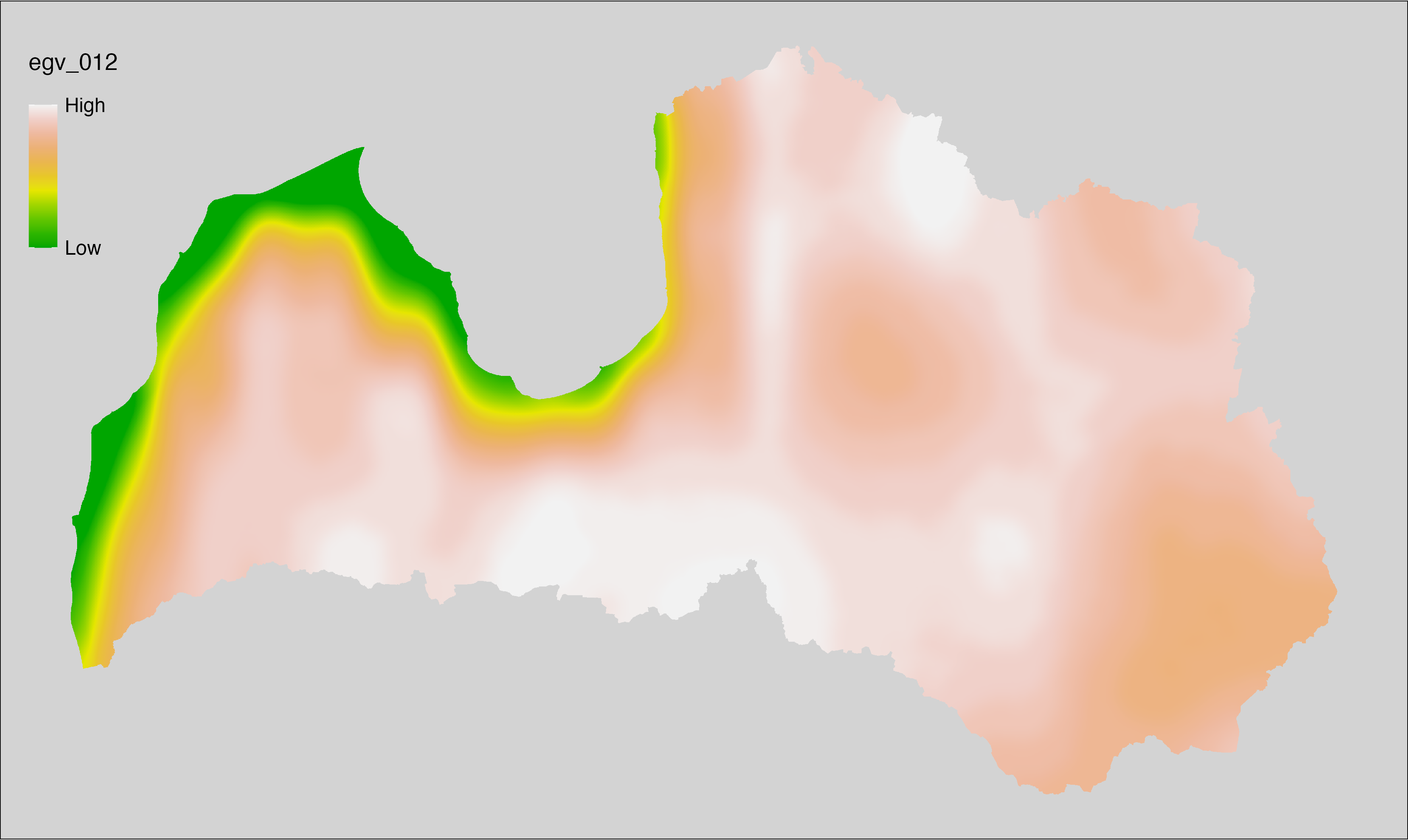
6.13 Climate_CHELSAv2.1-bio3_cell
filename: Climate_CHELSAv2.1-bio3_cell.tif
layername: egv_013
English name: Isothermality (ratio of diurnal variation to annual variation in air temperatures) (°C) (CHELSA v2.1) within the analysis cell (1 ha)
Latvian name: Izotermalitāte (attiecība starp diennakts un gada gaisa temperatūras svārstībām) (°C) (CHELSA v2.1) analīzes šūnā (1 ha)
Procedure: Directly follows CHELSA v2.1. EGV is prepared using
the workflow egvtools::downscale2egv() with inverse distance weighted (power =
2) gap filling and soft smoothing (power = 0.5) over 5 km radius around each cell.
Finally, the layer is standardised by subtracting the arithmetic mean and
dividing by the root mean squared error.
Code
# libs ----
if(!require(egvtools)) {remotes::install_github("aavotins/egvtools"); require(egvtools)}
# job ----
localname="Climate_CHELSAv2.1-bio3_cell.tif"
layername="egv_013"
reading="./Geodata/2024/CHELSA/Climate_CHELSAv2.1-bio3_cell.tif"
df <- downscale2egv(
template_path = "./Templates/TemplateRasters/LV100m_10km.tif",
grid_path = "./Templates/TemplateGrids/tikls1km_sauzeme.parquet",
rawfile_path = reading,
out_path = "./RasterGrids_100m/2024/RAW/",
file_name = localname,
layer_name = layername,
fill_gaps = TRUE,
smooth = TRUE,
smooth_radius_km = 5,
plot_result = TRUE)
print(df)
# standardisation ----
if(!require(terra)) {install.packages("terra"); require(terra)}
if(!require(tidyverse)) {install.packages("tidyverse"); require(tidyverse)}
nosaukums="Climate_CHELSAv2.1-bio3_cell.tif"
ielasisanas_cels=paste0("./RasterGrids_100m/2024/RAW/",nosaukums)
saglabasanas_cels=paste0("./RasterGrids_100m/2024/Scaled/",nosaukums)
slanis=rast(ielasisanas_cels)
videjais=global(slanis,fun="mean",na.rm=TRUE)
centrets=slanis-videjais[,1]
standartnovirze=terra::global(centrets,fun="rms",na.rm=TRUE)
merogots=centrets/standartnovirze[,1]
writeRaster(merogots,
filename=saglabasanas_cels,
overwrite=TRUE)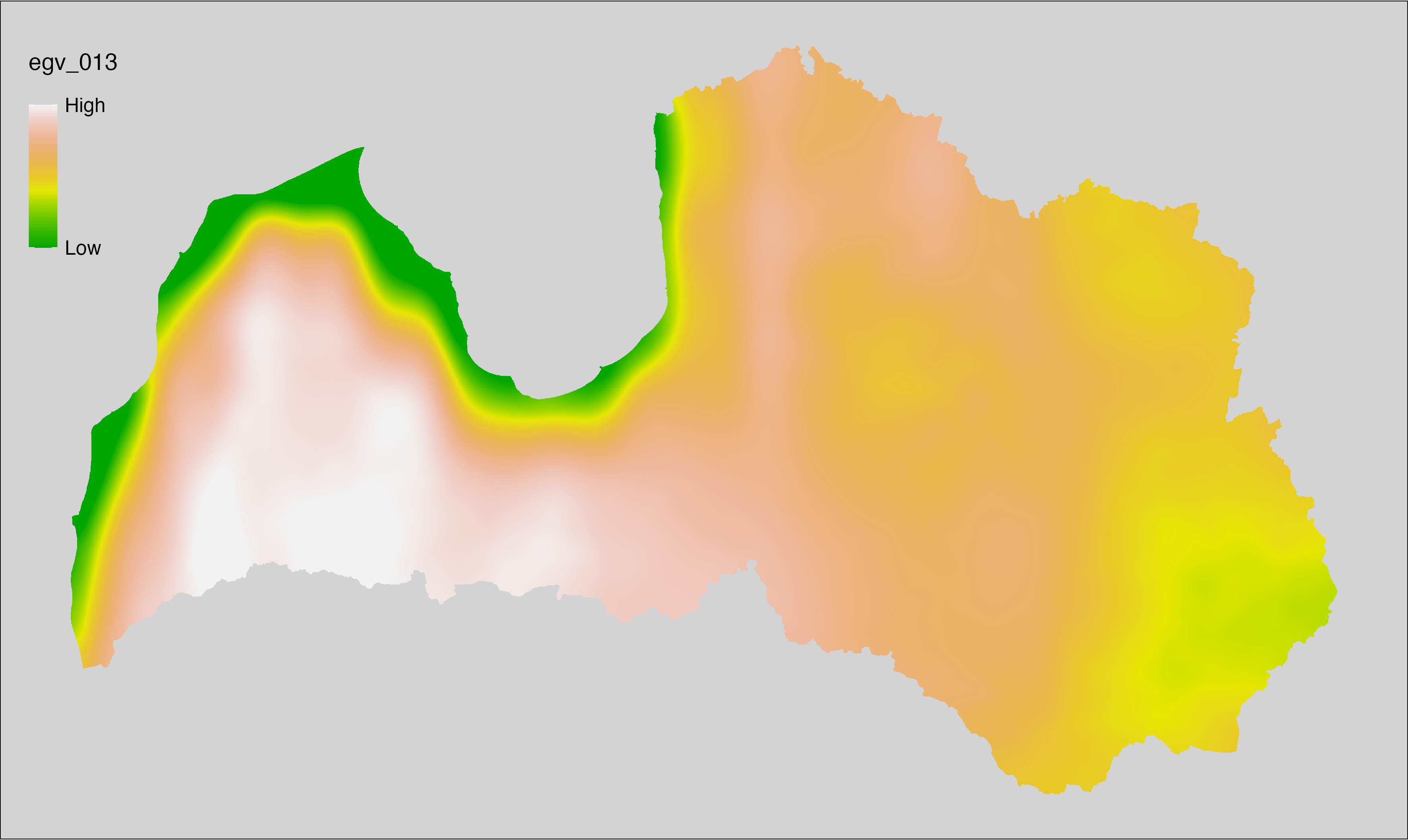
6.14 Climate_CHELSAv2.1-bio4_cell
filename: Climate_CHELSAv2.1-bio4_cell.tif
layername: egv_014
English name: Temperature seasonality (standard deviation of the monthly mean air temperatures) (°C/100) (CHELSA v2.1) within the analysis cell (1 ha)
Latvian name: Temperatūru sezonalitāte (mēneša vidējo gaisa temperatūru standartnovirze) (°C/100) (CHELSA v2.1) analīzes šūnā (1 ha)
Procedure: Directly follows CHELSA v2.1. EGV is prepared using
the workflow egvtools::downscale2egv() with inverse distance weighted (power =
2) gap filling and soft smoothing (power = 0.5) over 5 km radius around each cell.
Finally, the layer is standardised by subtracting the arithmetic mean and
dividing by the root mean squared error.
Code
# libs ----
if(!require(egvtools)) {remotes::install_github("aavotins/egvtools"); require(egvtools)}
# job ----
localname="Climate_CHELSAv2.1-bio4_cell.tif"
layername="egv_014"
reading="./Geodata/2024/CHELSA/Climate_CHELSAv2.1-bio4_cell.tif"
df <- downscale2egv(
template_path = "./Templates/TemplateRasters/LV100m_10km.tif",
grid_path = "./Templates/TemplateGrids/tikls1km_sauzeme.parquet",
rawfile_path = reading,
out_path = "./RasterGrids_100m/2024/RAW/",
file_name = localname,
layer_name = layername,
fill_gaps = TRUE,
smooth = TRUE,
smooth_radius_km = 5,
plot_result = TRUE)
print(df)
# standardisation ----
if(!require(terra)) {install.packages("terra"); require(terra)}
if(!require(tidyverse)) {install.packages("tidyverse"); require(tidyverse)}
nosaukums="Climate_CHELSAv2.1-bio4_cell.tif"
ielasisanas_cels=paste0("./RasterGrids_100m/2024/RAW/",nosaukums)
saglabasanas_cels=paste0("./RasterGrids_100m/2024/Scaled/",nosaukums)
slanis=rast(ielasisanas_cels)
videjais=global(slanis,fun="mean",na.rm=TRUE)
centrets=slanis-videjais[,1]
standartnovirze=terra::global(centrets,fun="rms",na.rm=TRUE)
merogots=centrets/standartnovirze[,1]
writeRaster(merogots,
filename=saglabasanas_cels,
overwrite=TRUE)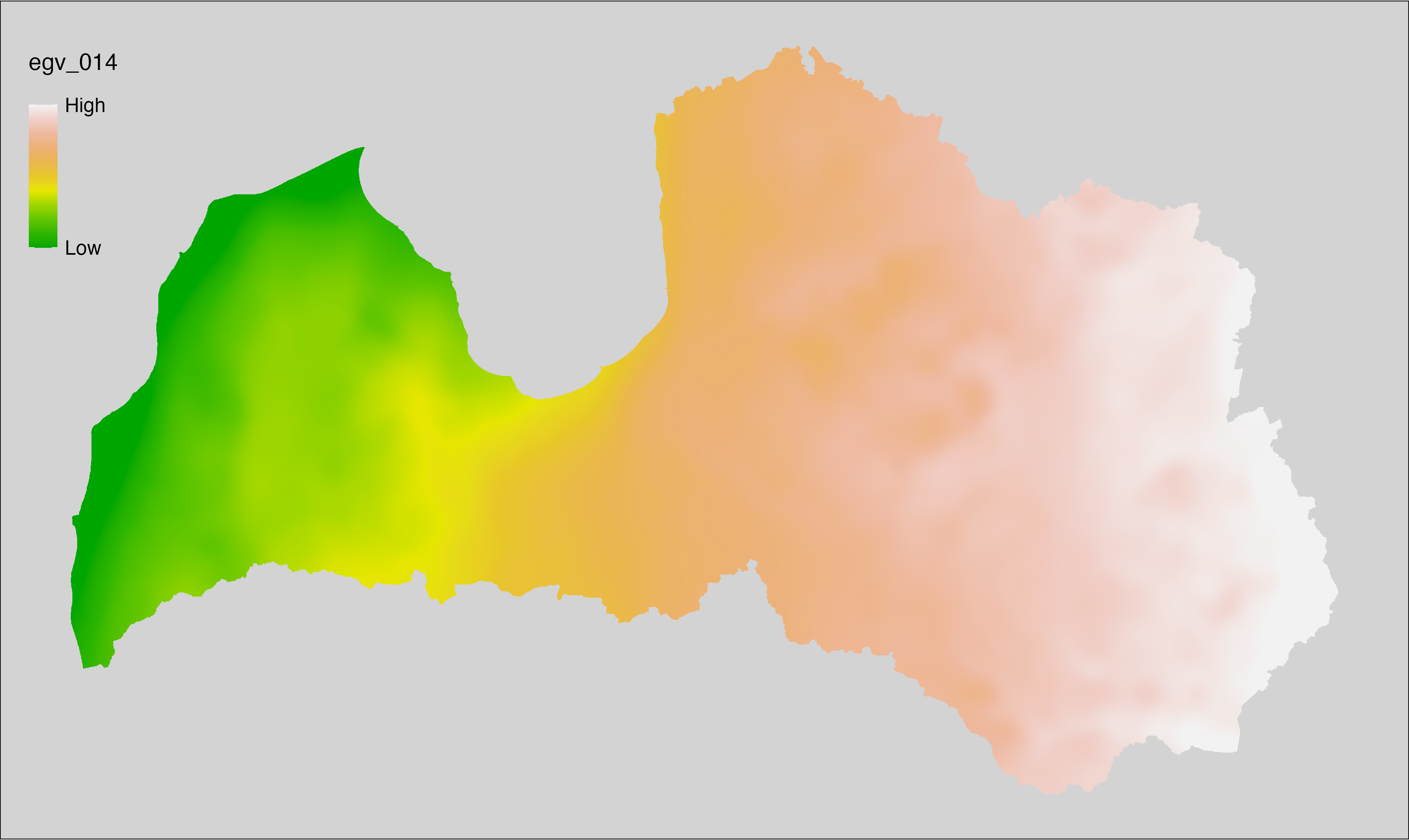
6.15 Climate_CHELSAv2.1-bio5_cell
filename: Climate_CHELSAv2.1-bio5_cell.tif
layername: egv_015
English name: Mean daily maximum air temperature (°C) of the warmest month (CHELSA v2.1) within the analysis cell (1 ha)
Latvian name: Siltākā mēneša vidējā ik dienas augstākā gaisa temperatūra (°C) (CHELSA v2.1) analīzes šūnā (1 ha)
Procedure: Directly follows CHELSA v2.1. EGV is prepared using
the workflow egvtools::downscale2egv() with inverse distance weighted (power =
2) gap filling and soft smoothing (power = 0.5) over 5 km radius around each cell.
Finally, the layer is standardised by subtracting the arithmetic mean and
dividing by the root mean squared error.
Code
# libs ----
if(!require(egvtools)) {remotes::install_github("aavotins/egvtools"); require(egvtools)}
# job ----
localname="Climate_CHELSAv2.1-bio5_cell.tif"
layername="egv_015"
reading="./Geodata/2024/CHELSA/Climate_CHELSAv2.1-bio5_cell.tif"
df <- downscale2egv(
template_path = "./Templates/TemplateRasters/LV100m_10km.tif",
grid_path = "./Templates/TemplateGrids/tikls1km_sauzeme.parquet",
rawfile_path = reading,
out_path = "./RasterGrids_100m/2024/RAW/",
file_name = localname,
layer_name = layername,
fill_gaps = TRUE,
smooth = TRUE,
smooth_radius_km = 5,
plot_result = TRUE)
print(df)
# standardisation ----
if(!require(terra)) {install.packages("terra"); require(terra)}
if(!require(tidyverse)) {install.packages("tidyverse"); require(tidyverse)}
nosaukums="Climate_CHELSAv2.1-bio5_cell.tif"
ielasisanas_cels=paste0("./RasterGrids_100m/2024/RAW/",nosaukums)
saglabasanas_cels=paste0("./RasterGrids_100m/2024/Scaled/",nosaukums)
slanis=rast(ielasisanas_cels)
videjais=global(slanis,fun="mean",na.rm=TRUE)
centrets=slanis-videjais[,1]
standartnovirze=terra::global(centrets,fun="rms",na.rm=TRUE)
merogots=centrets/standartnovirze[,1]
writeRaster(merogots,
filename=saglabasanas_cels,
overwrite=TRUE)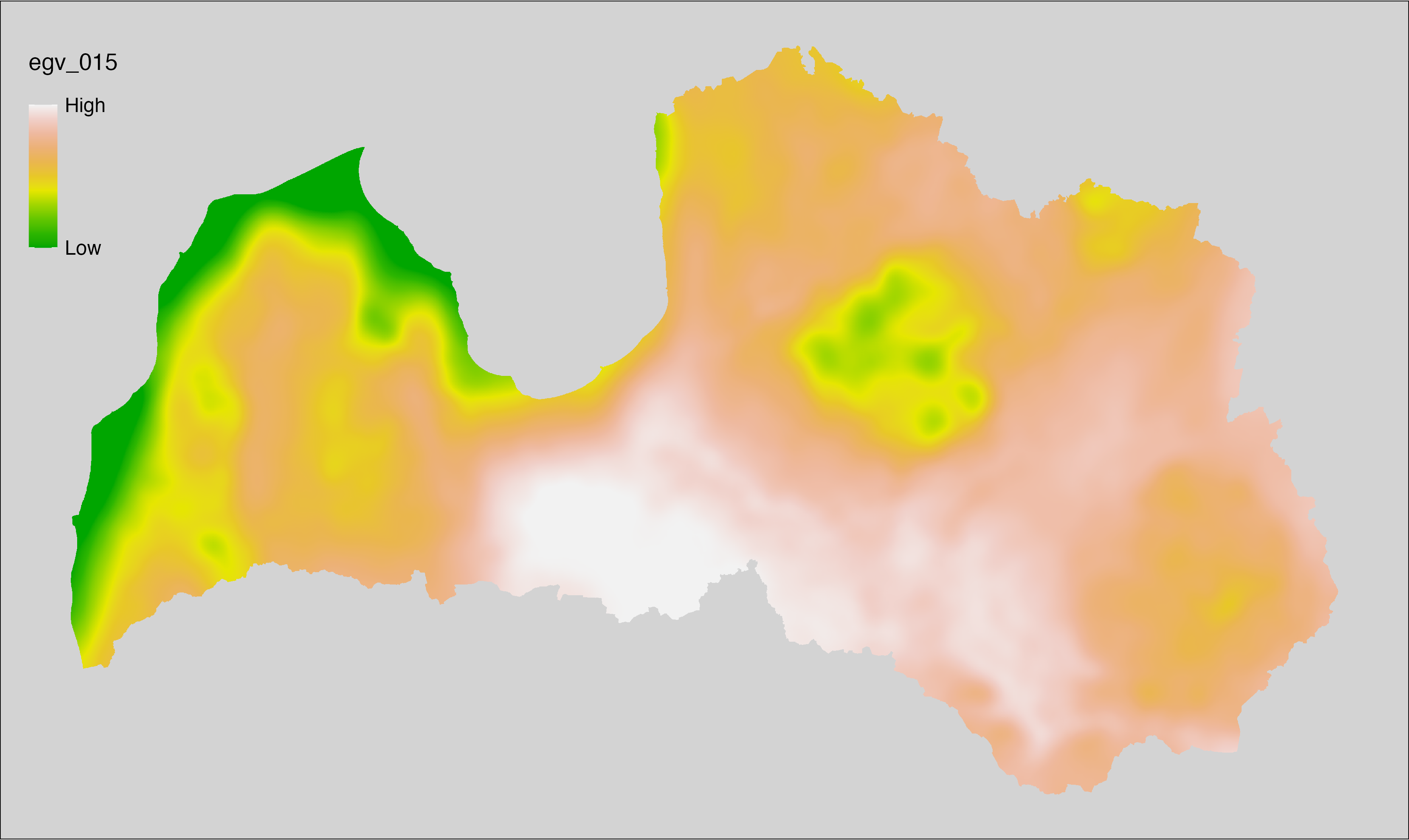
6.16 Climate_CHELSAv2.1-bio6_cell
filename: Climate_CHELSAv2.1-bio6_cell.tif
layername: egv_016
English name: Mean daily minimum air temperature (°C) of the coldest month (CHELSA v2.1) within the analysis cell (1 ha)
Latvian name: Aukstākā mēneša vidējā ik dienas zemākā gaisa temperatūra (°C) (CHELSA v2.1) analīzes šūnā (1 ha)
Procedure: Directly follows CHELSA v2.1. EGV is prepared using
the workflow egvtools::downscale2egv() with inverse distance weighted (power =
2) gap filling and soft smoothing (power = 0.5) over 5 km radius around each cell.
Finally, the layer is standardised by subtracting the arithmetic mean and
dividing by the root mean squared error.
Code
# libs ----
if(!require(egvtools)) {remotes::install_github("aavotins/egvtools"); require(egvtools)}
# job ----
localname="Climate_CHELSAv2.1-bio6_cell.tif"
layername="egv_016"
reading="./Geodata/2024/CHELSA/Climate_CHELSAv2.1-bio6_cell.tif"
df <- downscale2egv(
template_path = "./Templates/TemplateRasters/LV100m_10km.tif",
grid_path = "./Templates/TemplateGrids/tikls1km_sauzeme.parquet",
rawfile_path = reading,
out_path = "./RasterGrids_100m/2024/RAW/",
file_name = localname,
layer_name = layername,
fill_gaps = TRUE,
smooth = TRUE,
smooth_radius_km = 5,
plot_result = TRUE)
print(df)
# standardisation ----
if(!require(terra)) {install.packages("terra"); require(terra)}
if(!require(tidyverse)) {install.packages("tidyverse"); require(tidyverse)}
nosaukums="Climate_CHELSAv2.1-bio6_cell.tif"
ielasisanas_cels=paste0("./RasterGrids_100m/2024/RAW/",nosaukums)
saglabasanas_cels=paste0("./RasterGrids_100m/2024/Scaled/",nosaukums)
slanis=rast(ielasisanas_cels)
videjais=global(slanis,fun="mean",na.rm=TRUE)
centrets=slanis-videjais[,1]
standartnovirze=terra::global(centrets,fun="rms",na.rm=TRUE)
merogots=centrets/standartnovirze[,1]
writeRaster(merogots,
filename=saglabasanas_cels,
overwrite=TRUE)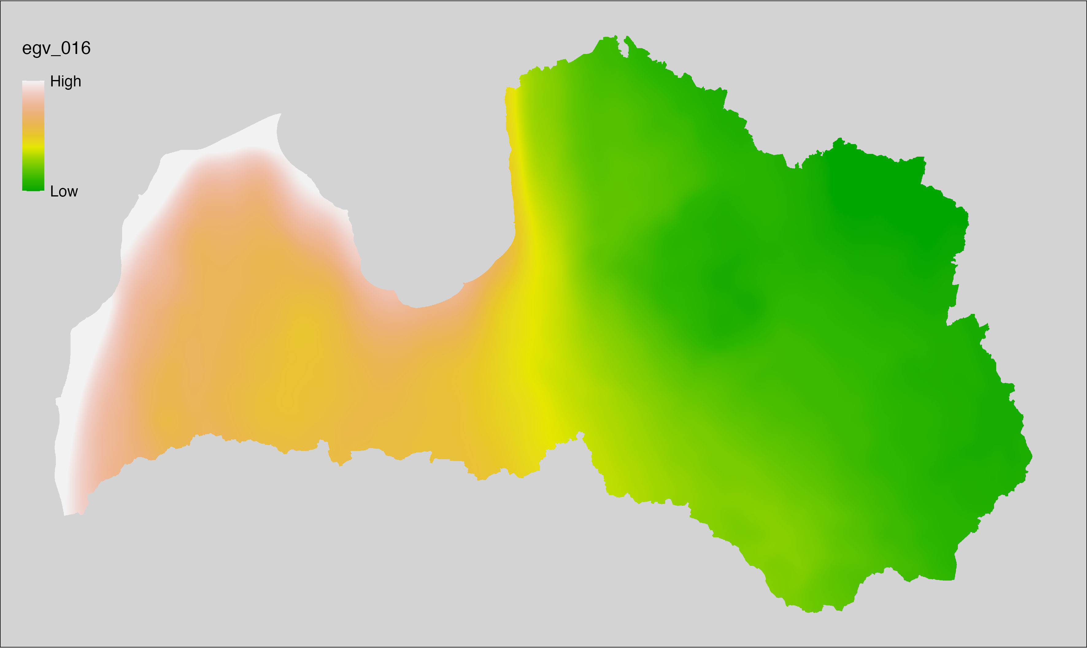
6.17 Climate_CHELSAv2.1-bio7_cell
filename: Climate_CHELSAv2.1-bio7_cell.tif
layername: egv_017
English name: Annual range of air temperature (°C) (CHELSA v2.1) within the analysis cell (1 ha)
Latvian name: Gada gaisa temperatūru amplitūda (°C) (CHELSA v2.1) analīzes šūnā (1 ha)
Procedure: Directly follows CHELSA v2.1. EGV is prepared using
the workflow egvtools::downscale2egv() with inverse distance weighted (power =
2) gap filling and soft smoothing (power = 0.5) over 5 km radius around each cell.
Finally, the layer is standardised by subtracting the arithmetic mean and
dividing by the root mean squared error.
Code
# libs ----
if(!require(egvtools)) {remotes::install_github("aavotins/egvtools"); require(egvtools)}
# job ----
localname="Climate_CHELSAv2.1-bio7_cell.tif"
layername="egv_017"
reading="./Geodata/2024/CHELSA/Climate_CHELSAv2.1-bio7_cell.tif"
df <- downscale2egv(
template_path = "./Templates/TemplateRasters/LV100m_10km.tif",
grid_path = "./Templates/TemplateGrids/tikls1km_sauzeme.parquet",
rawfile_path = reading,
out_path = "./RasterGrids_100m/2024/RAW/",
file_name = localname,
layer_name = layername,
fill_gaps = TRUE,
smooth = TRUE,
smooth_radius_km = 5,
plot_result = TRUE)
print(df)
# standardisation ----
if(!require(terra)) {install.packages("terra"); require(terra)}
if(!require(tidyverse)) {install.packages("tidyverse"); require(tidyverse)}
nosaukums="Climate_CHELSAv2.1-bio7_cell.tif"
ielasisanas_cels=paste0("./RasterGrids_100m/2024/RAW/",nosaukums)
saglabasanas_cels=paste0("./RasterGrids_100m/2024/Scaled/",nosaukums)
slanis=rast(ielasisanas_cels)
videjais=global(slanis,fun="mean",na.rm=TRUE)
centrets=slanis-videjais[,1]
standartnovirze=terra::global(centrets,fun="rms",na.rm=TRUE)
merogots=centrets/standartnovirze[,1]
writeRaster(merogots,
filename=saglabasanas_cels,
overwrite=TRUE)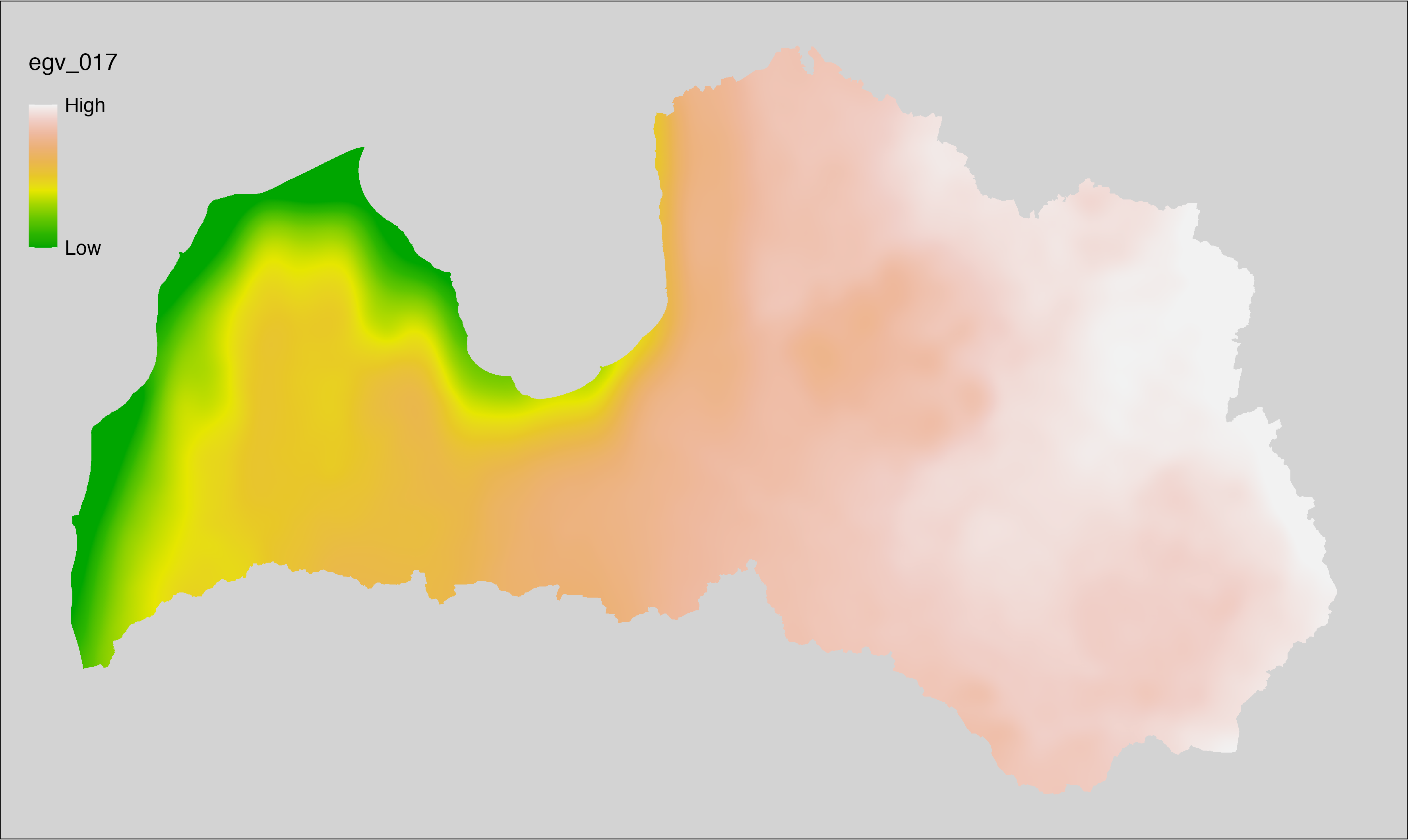
6.18 Climate_CHELSAv2.1-bio8_cell
filename: Climate_CHELSAv2.1-bio8_cell.tif
layername: egv_018
English name: Mean daily mean air temperatures (°C) of the wettest quarter (CHELSA v2.1) within the analysis cell (1 ha)
Latvian name: Slapjākā ceturkšņa vidējā ik dienas vidējā gaisa temperatūra (°C) (CHELSA v2.1) analīzes šūnā (1 ha)
Procedure: Directly follows CHELSA v2.1. EGV is prepared using
the workflow egvtools::downscale2egv() with inverse distance weighted (power =
2) gap filling and soft smoothing (power = 0.5) over 5 km radius around each cell.
Finally, the layer is standardised by subtracting the arithmetic mean and
dividing by the root mean squared error.
Code
# libs ----
if(!require(egvtools)) {remotes::install_github("aavotins/egvtools"); require(egvtools)}
# job ----
localname="Climate_CHELSAv2.1-bio8_cell.tif"
layername="egv_018"
reading="./Geodata/2024/CHELSA/Climate_CHELSAv2.1-bio8_cell.tif"
df <- downscale2egv(
template_path = "./Templates/TemplateRasters/LV100m_10km.tif",
grid_path = "./Templates/TemplateGrids/tikls1km_sauzeme.parquet",
rawfile_path = reading,
out_path = "./RasterGrids_100m/2024/RAW/",
file_name = localname,
layer_name = layername,
fill_gaps = TRUE,
smooth = TRUE,
smooth_radius_km = 5,
plot_result = TRUE)
print(df)
# standardisation ----
if(!require(terra)) {install.packages("terra"); require(terra)}
if(!require(tidyverse)) {install.packages("tidyverse"); require(tidyverse)}
nosaukums="Climate_CHELSAv2.1-bio8_cell.tif"
ielasisanas_cels=paste0("./RasterGrids_100m/2024/RAW/",nosaukums)
saglabasanas_cels=paste0("./RasterGrids_100m/2024/Scaled/",nosaukums)
slanis=rast(ielasisanas_cels)
videjais=global(slanis,fun="mean",na.rm=TRUE)
centrets=slanis-videjais[,1]
standartnovirze=terra::global(centrets,fun="rms",na.rm=TRUE)
merogots=centrets/standartnovirze[,1]
writeRaster(merogots,
filename=saglabasanas_cels,
overwrite=TRUE)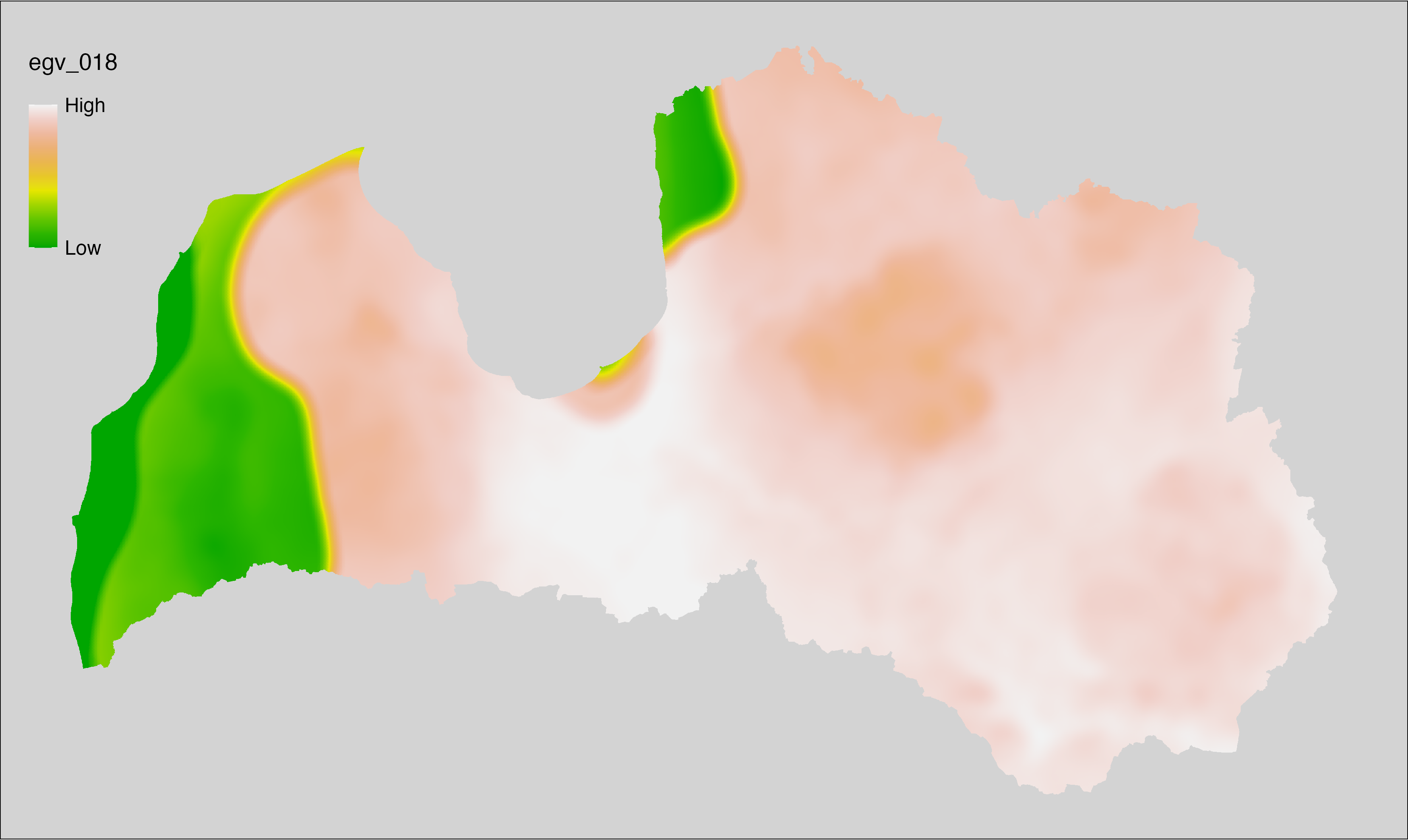
6.19 Climate_CHELSAv2.1-bio9_cell
filename: Climate_CHELSAv2.1-bio9_cell.tif
layername: egv_019
English name: Mean daily mean air temperatures (°C) of the driest quarter (CHELSA v2.1) within the analysis cell (1 ha)
Latvian name: Sausākā ceturkšņa vidējā ik dienas vidējā gaisa temperatūra (°C) (CHELSA v2.1) analīzes šūnā (1 ha)
Procedure: Directly follows CHELSA v2.1. EGV is prepared using
the workflow egvtools::downscale2egv() with inverse distance weighted (power =
2) gap filling and soft smoothing (power = 0.5) over 5 km radius around each cell.
Finally, the layer is standardised by subtracting the arithmetic mean and
dividing by the root mean squared error.
Code
# libs ----
if(!require(egvtools)) {remotes::install_github("aavotins/egvtools"); require(egvtools)}
# job ----
localname="Climate_CHELSAv2.1-bio9_cell.tif"
layername="egv_019"
reading="./Geodata/2024/CHELSA/Climate_CHELSAv2.1-bio9_cell.tif"
df <- downscale2egv(
template_path = "./Templates/TemplateRasters/LV100m_10km.tif",
grid_path = "./Templates/TemplateGrids/tikls1km_sauzeme.parquet",
rawfile_path = reading,
out_path = "./RasterGrids_100m/2024/RAW/",
file_name = localname,
layer_name = layername,
fill_gaps = TRUE,
smooth = TRUE,
smooth_radius_km = 5,
plot_result = TRUE)
print(df)
# standardisation ----
if(!require(terra)) {install.packages("terra"); require(terra)}
if(!require(tidyverse)) {install.packages("tidyverse"); require(tidyverse)}
nosaukums="Climate_CHELSAv2.1-bio9_cell.tif"
ielasisanas_cels=paste0("./RasterGrids_100m/2024/RAW/",nosaukums)
saglabasanas_cels=paste0("./RasterGrids_100m/2024/Scaled/",nosaukums)
slanis=rast(ielasisanas_cels)
videjais=global(slanis,fun="mean",na.rm=TRUE)
centrets=slanis-videjais[,1]
standartnovirze=terra::global(centrets,fun="rms",na.rm=TRUE)
merogots=centrets/standartnovirze[,1]
writeRaster(merogots,
filename=saglabasanas_cels,
overwrite=TRUE)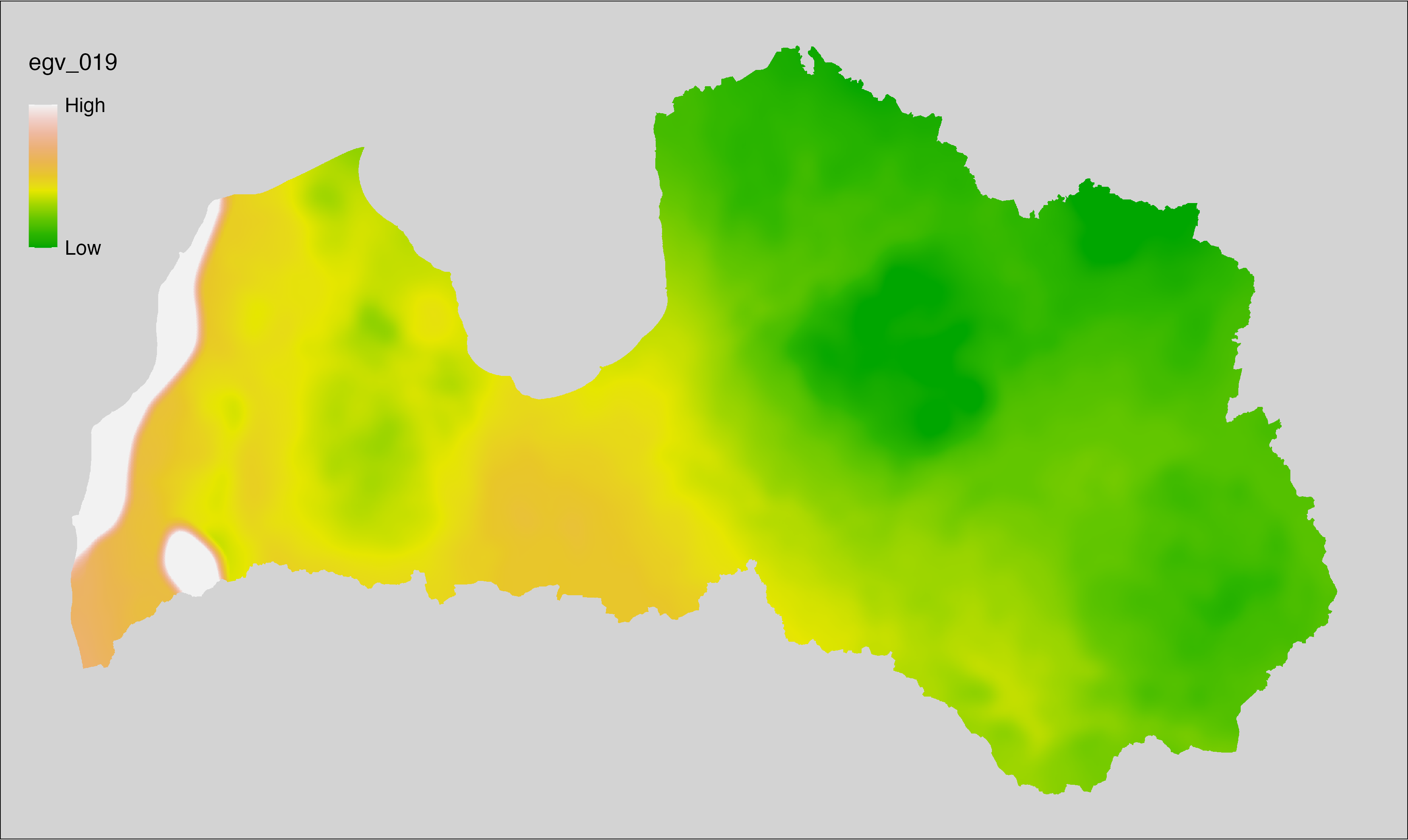
6.20 Climate_CHELSAv2.1-clt-max_cell
filename: Climate_CHELSAv2.1-clt-max_cell.tif
layername: egv_020
English name: Mean of monthly maximum cloud area fraction (%) (CHELSA v2.1) within the analysis cell (1 ha)
Latvian name: Mēneša maksimumu vidējais mākoņu segums (%) (CHELSA v2.1) analīzes šūnā (1 ha)
Procedure: Directly follows CHELSA v2.1. EGV is prepared using
the workflow egvtools::downscale2egv() with inverse distance weighted (power =
2) gap filling and soft smoothing (power = 0.5) over 5 km radius around each cell.
Finally, the layer is standardised by subtracting the arithmetic mean and
dividing by the root mean squared error.
Code
# libs ----
if(!require(egvtools)) {remotes::install_github("aavotins/egvtools"); require(egvtools)}
# job ----
localname="Climate_CHELSAv2.1-clt-max_cell.tif"
layername="egv_020"
reading="./Geodata/2024/CHELSA/Climate_CHELSAv2.1-clt-max_cell.tif"
df <- downscale2egv(
template_path = "./Templates/TemplateRasters/LV100m_10km.tif",
grid_path = "./Templates/TemplateGrids/tikls1km_sauzeme.parquet",
rawfile_path = reading,
out_path = "./RasterGrids_100m/2024/RAW/",
file_name = localname,
layer_name = layername,
fill_gaps = TRUE,
smooth = TRUE,
smooth_radius_km = 5,
plot_result = TRUE)
print(df)
# standardisation ----
if(!require(terra)) {install.packages("terra"); require(terra)}
if(!require(tidyverse)) {install.packages("tidyverse"); require(tidyverse)}
nosaukums="Climate_CHELSAv2.1-clt-max_cell.tif"
ielasisanas_cels=paste0("./RasterGrids_100m/2024/RAW/",nosaukums)
saglabasanas_cels=paste0("./RasterGrids_100m/2024/Scaled/",nosaukums)
slanis=rast(ielasisanas_cels)
videjais=global(slanis,fun="mean",na.rm=TRUE)
centrets=slanis-videjais[,1]
standartnovirze=terra::global(centrets,fun="rms",na.rm=TRUE)
merogots=centrets/standartnovirze[,1]
writeRaster(merogots,
filename=saglabasanas_cels,
overwrite=TRUE)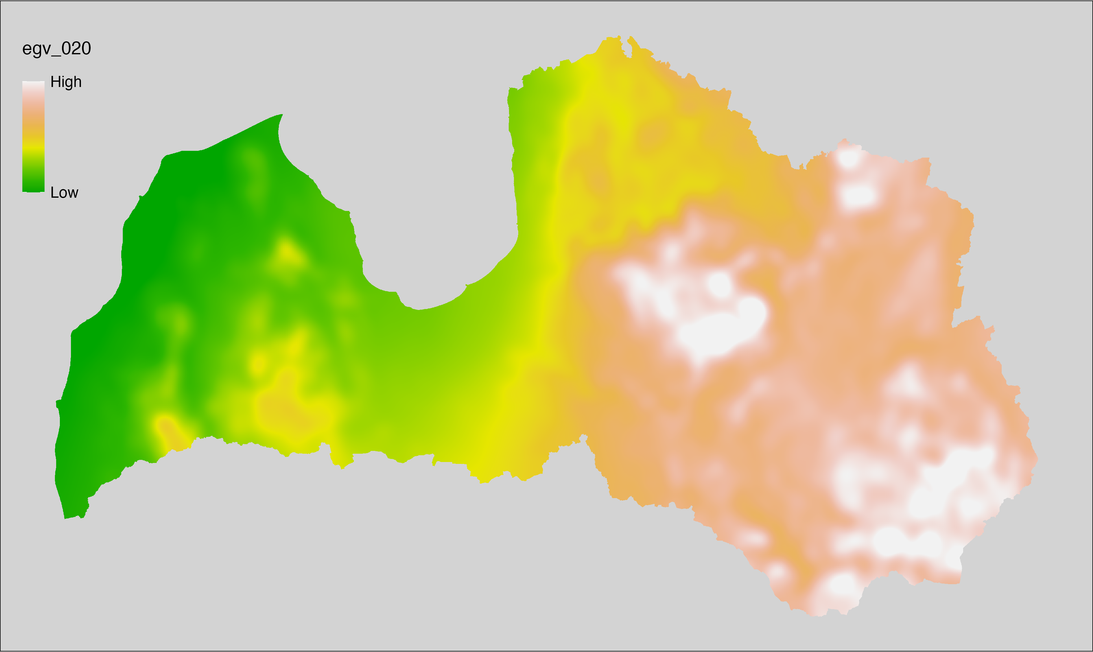
6.21 Climate_CHELSAv2.1-clt-mean_cell
filename: Climate_CHELSAv2.1-clt-mean_cell.tif
layername: egv_021
English name: Mean monthly mean cloud area fraction (%) (CHELSA v2.1) within the analysis cell (1 ha)
Latvian name: Vidējais ik mēneša vidējais mākoņu segums (%) (CHELSA v2.1) analīzes šūnā (1 ha)
Procedure: Directly follows CHELSA v2.1. EGV is prepared using
the workflow egvtools::downscale2egv() with inverse distance weighted (power =
2) gap filling and soft smoothing (power = 0.5) over 5 km radius around each cell.
Finally, the layer is standardised by subtracting the arithmetic mean and
dividing by the root mean squared error.
Code
# libs ----
if(!require(egvtools)) {remotes::install_github("aavotins/egvtools"); require(egvtools)}
# job ----
localname="Climate_CHELSAv2.1-clt-mean_cell.tif"
layername="egv_021"
reading="./Geodata/2024/CHELSA/Climate_CHELSAv2.1-clt-mean_cell.tif"
df <- downscale2egv(
template_path = "./Templates/TemplateRasters/LV100m_10km.tif",
grid_path = "./Templates/TemplateGrids/tikls1km_sauzeme.parquet",
rawfile_path = reading,
out_path = "./RasterGrids_100m/2024/RAW/",
file_name = localname,
layer_name = layername,
fill_gaps = TRUE,
smooth = TRUE,
smooth_radius_km = 5,
plot_result = TRUE)
print(df)
# standardisation ----
if(!require(terra)) {install.packages("terra"); require(terra)}
if(!require(tidyverse)) {install.packages("tidyverse"); require(tidyverse)}
nosaukums="Climate_CHELSAv2.1-clt-mean_cell.tif"
ielasisanas_cels=paste0("./RasterGrids_100m/2024/RAW/",nosaukums)
saglabasanas_cels=paste0("./RasterGrids_100m/2024/Scaled/",nosaukums)
slanis=rast(ielasisanas_cels)
videjais=global(slanis,fun="mean",na.rm=TRUE)
centrets=slanis-videjais[,1]
standartnovirze=terra::global(centrets,fun="rms",na.rm=TRUE)
merogots=centrets/standartnovirze[,1]
writeRaster(merogots,
filename=saglabasanas_cels,
overwrite=TRUE)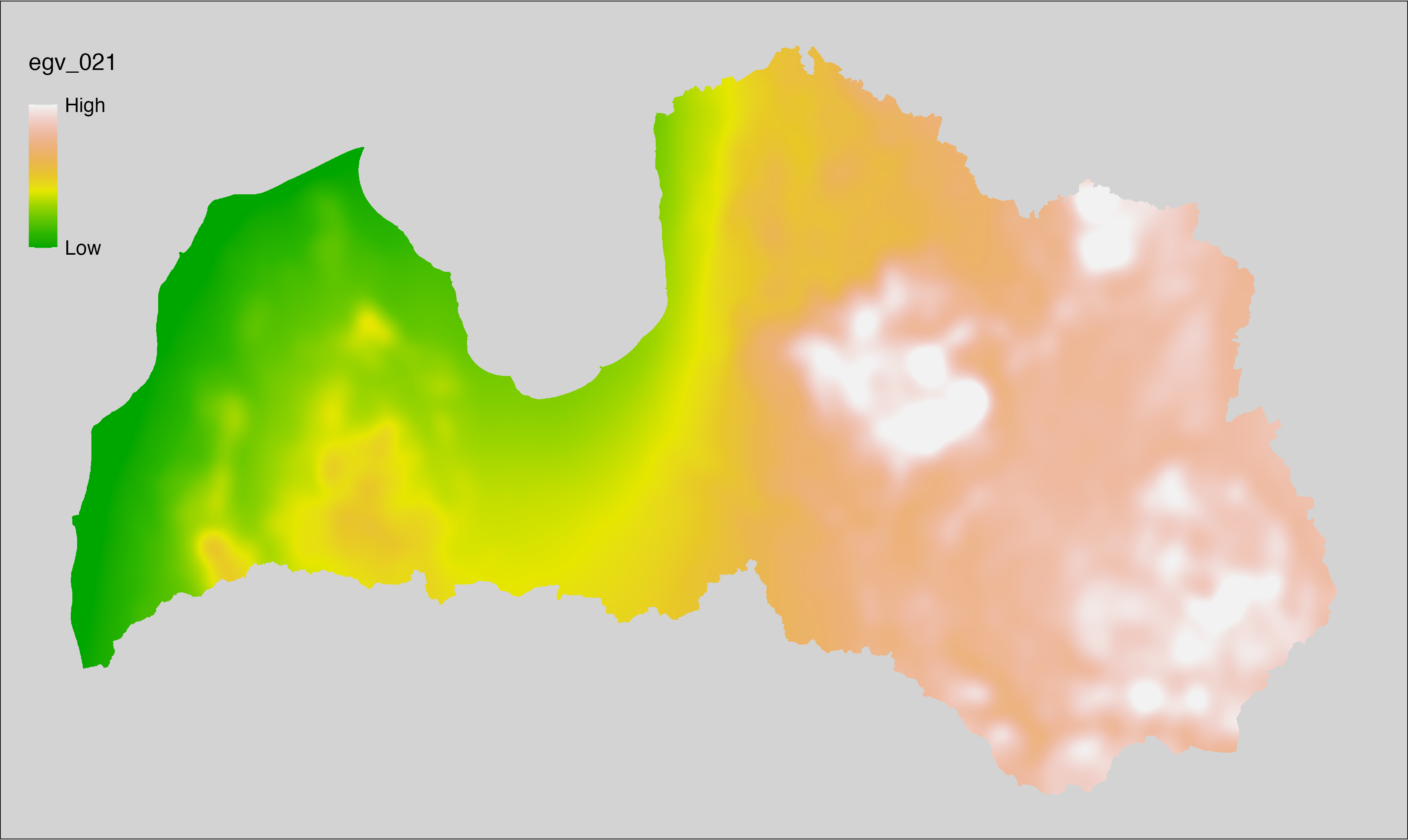
6.22 Climate_CHELSAv2.1-clt-min_cell
filename: Climate_CHELSAv2.1-clt-min_cell.tif
layername: egv_022
English name: Mean of monthly minimum cloud area fraction (%) (CHELSA v2.1) within the analysis cell (1 ha)
Latvian name: Mēneša minimumu vidējais mākoņu segums (%) (CHELSA v2.1) analīzes šūnā (1 ha)
Procedure: Directly follows CHELSA v2.1. EGV is prepared using
the workflow egvtools::downscale2egv() with inverse distance weighted (power =
2) gap filling and soft smoothing (power = 0.5) over 5 km radius around each cell.
Finally, the layer is standardised by subtracting the arithmetic mean and
dividing by the root mean squared error.
Code
# libs ----
if(!require(egvtools)) {remotes::install_github("aavotins/egvtools"); require(egvtools)}
# job ----
localname="Climate_CHELSAv2.1-clt-min_cell.tif"
layername="egv_022"
reading="./Geodata/2024/CHELSA/Climate_CHELSAv2.1-clt-min_cell.tif"
df <- downscale2egv(
template_path = "./Templates/TemplateRasters/LV100m_10km.tif",
grid_path = "./Templates/TemplateGrids/tikls1km_sauzeme.parquet",
rawfile_path = reading,
out_path = "./RasterGrids_100m/2024/RAW/",
file_name = localname,
layer_name = layername,
fill_gaps = TRUE,
smooth = TRUE,
smooth_radius_km = 5,
plot_result = TRUE)
print(df)
# standardisation ----
if(!require(terra)) {install.packages("terra"); require(terra)}
if(!require(tidyverse)) {install.packages("tidyverse"); require(tidyverse)}
nosaukums="Climate_CHELSAv2.1-clt-min_cell.tif"
ielasisanas_cels=paste0("./RasterGrids_100m/2024/RAW/",nosaukums)
saglabasanas_cels=paste0("./RasterGrids_100m/2024/Scaled/",nosaukums)
slanis=rast(ielasisanas_cels)
videjais=global(slanis,fun="mean",na.rm=TRUE)
centrets=slanis-videjais[,1]
standartnovirze=terra::global(centrets,fun="rms",na.rm=TRUE)
merogots=centrets/standartnovirze[,1]
writeRaster(merogots,
filename=saglabasanas_cels,
overwrite=TRUE)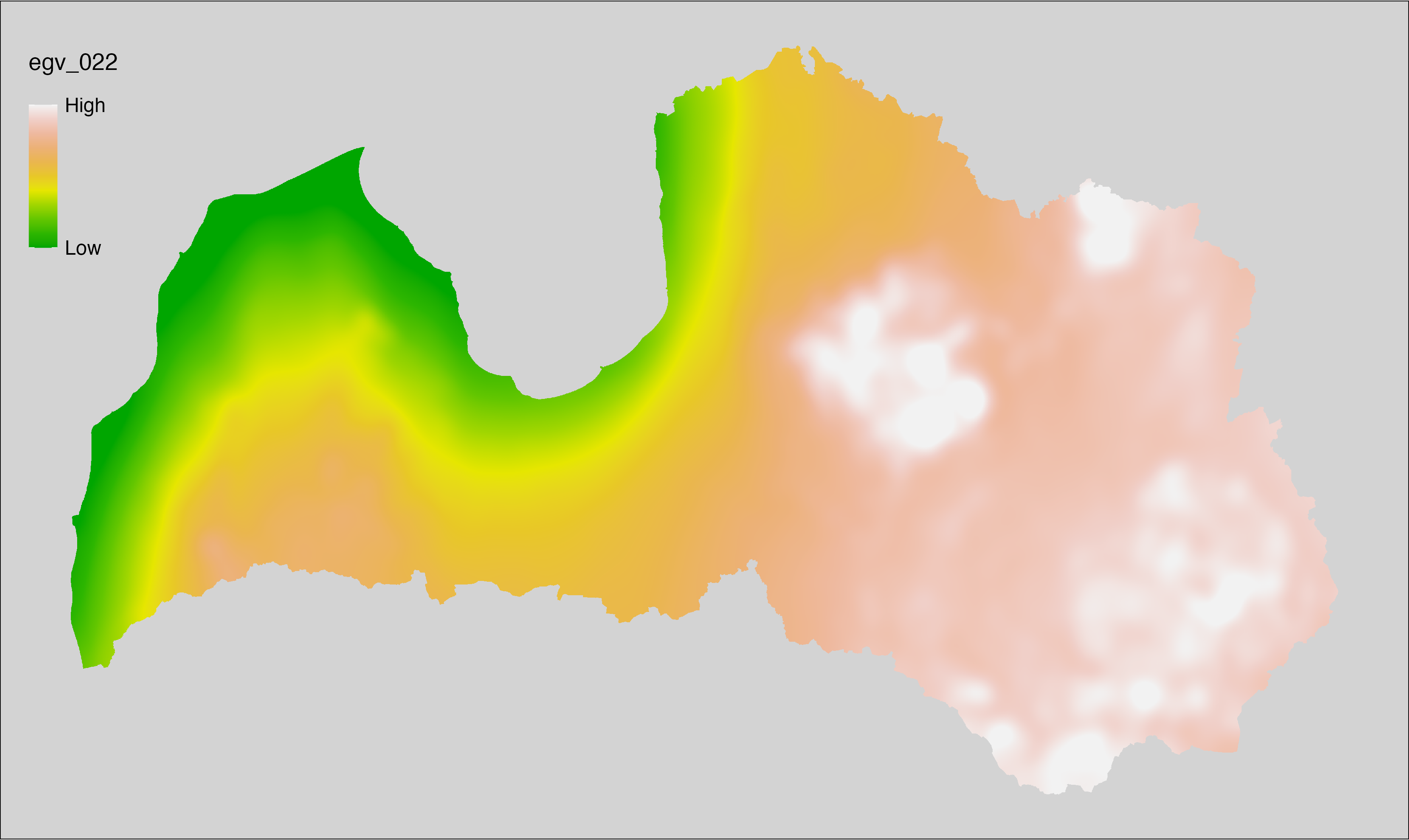
6.23 Climate_CHELSAv2.1-clt-range_cell
filename: Climate_CHELSAv2.1-clt-range_cell.tif
layername: egv_023
English name: Annual range of monthly cloud area fraction (%) (CHELSA v2.1) within the analysis cell (1 ha)
Latvian name: Gada mākoņu seguma amplitūda (%) (CHELSA v2.1) analīzes šūnā (1 ha)
Procedure: Directly follows CHELSA v2.1. EGV is prepared using
the workflow egvtools::downscale2egv() with inverse distance weighted (power =
2) gap filling and soft smoothing (power = 0.5) over 5 km radius around each cell.
Finally, the layer is standardised by subtracting the arithmetic mean and
dividing by the root mean squared error.
Code
# libs ----
if(!require(egvtools)) {remotes::install_github("aavotins/egvtools"); require(egvtools)}
# job ----
localname="Climate_CHELSAv2.1-clt-range_cell.tif"
layername="egv_023"
reading="./Geodata/2024/CHELSA/Climate_CHELSAv2.1-clt-range_cell.tif"
df <- downscale2egv(
template_path = "./Templates/TemplateRasters/LV100m_10km.tif",
grid_path = "./Templates/TemplateGrids/tikls1km_sauzeme.parquet",
rawfile_path = reading,
out_path = "./RasterGrids_100m/2024/RAW/",
file_name = localname,
layer_name = layername,
fill_gaps = TRUE,
smooth = TRUE,
smooth_radius_km = 5,
plot_result = TRUE)
print(df)
# standardisation ----
if(!require(terra)) {install.packages("terra"); require(terra)}
if(!require(tidyverse)) {install.packages("tidyverse"); require(tidyverse)}
nosaukums="Climate_CHELSAv2.1-clt-range_cell.tif"
ielasisanas_cels=paste0("./RasterGrids_100m/2024/RAW/",nosaukums)
saglabasanas_cels=paste0("./RasterGrids_100m/2024/Scaled/",nosaukums)
slanis=rast(ielasisanas_cels)
videjais=global(slanis,fun="mean",na.rm=TRUE)
centrets=slanis-videjais[,1]
standartnovirze=terra::global(centrets,fun="rms",na.rm=TRUE)
merogots=centrets/standartnovirze[,1]
writeRaster(merogots,
filename=saglabasanas_cels,
overwrite=TRUE)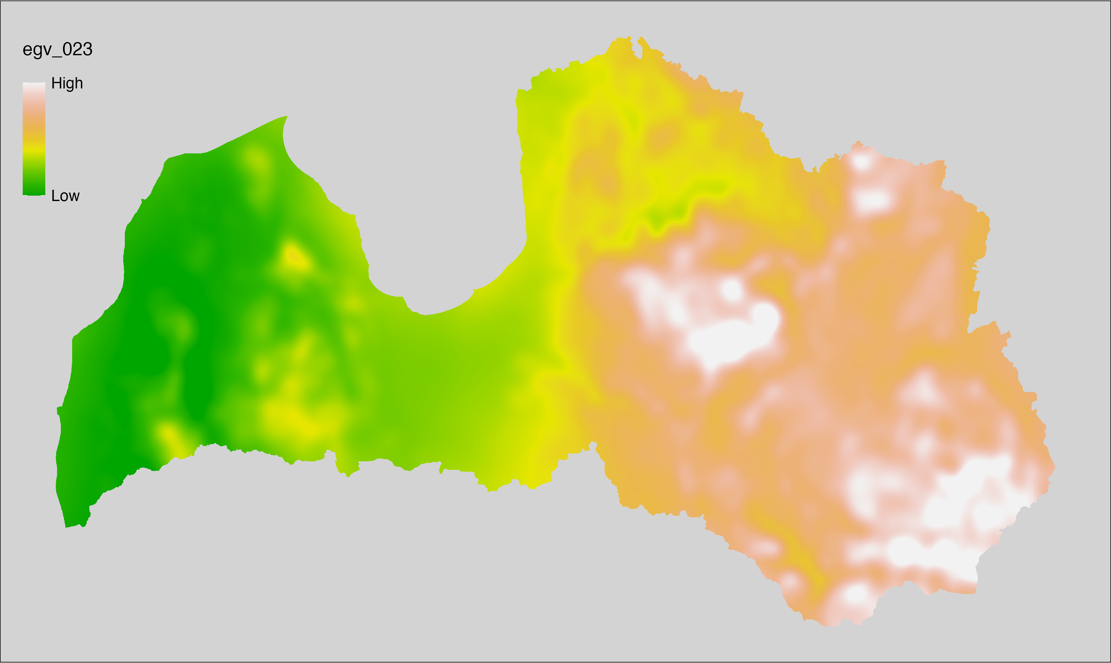
6.24 Climate_CHELSAv2.1-cmi-max_cell
filename: Climate_CHELSAv2.1-cmi-max_cell.tif
layername: egv_024
English name: Mean of monthly maximum climate moisture index (kg m⁻² month⁻¹) (CHELSA v2.1) within the analysis cell (1 ha)
Latvian name: Vidējais ik mēneša maksimālais klimata mitruma indekss (kg m⁻² month⁻¹) (CHELSA v2.1) analīzes šūnā (1 ha)
Procedure: Directly follows CHELSA v2.1. EGV is prepared using
the workflow egvtools::downscale2egv() with inverse distance weighted (power =
2) gap filling and soft smoothing (power = 0.5) over 5 km radius around each cell.
Finally, the layer is standardised by subtracting the arithmetic mean and
dividing by the root mean squared error.
Code
# libs ----
if(!require(egvtools)) {remotes::install_github("aavotins/egvtools"); require(egvtools)}
# job ----
localname="Climate_CHELSAv2.1-cmi-max_cell.tif"
layername="egv_024"
reading="./Geodata/2024/CHELSA/Climate_CHELSAv2.1-cmi-max_cell.tif"
df <- downscale2egv(
template_path = "./Templates/TemplateRasters/LV100m_10km.tif",
grid_path = "./Templates/TemplateGrids/tikls1km_sauzeme.parquet",
rawfile_path = reading,
out_path = "./RasterGrids_100m/2024/RAW/",
file_name = localname,
layer_name = layername,
fill_gaps = TRUE,
smooth = TRUE,
smooth_radius_km = 5,
plot_result = TRUE)
print(df)
# standardisation ----
if(!require(terra)) {install.packages("terra"); require(terra)}
if(!require(tidyverse)) {install.packages("tidyverse"); require(tidyverse)}
nosaukums="Climate_CHELSAv2.1-cmi-max_cell.tif"
ielasisanas_cels=paste0("./RasterGrids_100m/2024/RAW/",nosaukums)
saglabasanas_cels=paste0("./RasterGrids_100m/2024/Scaled/",nosaukums)
slanis=rast(ielasisanas_cels)
videjais=global(slanis,fun="mean",na.rm=TRUE)
centrets=slanis-videjais[,1]
standartnovirze=terra::global(centrets,fun="rms",na.rm=TRUE)
merogots=centrets/standartnovirze[,1]
writeRaster(merogots,
filename=saglabasanas_cels,
overwrite=TRUE)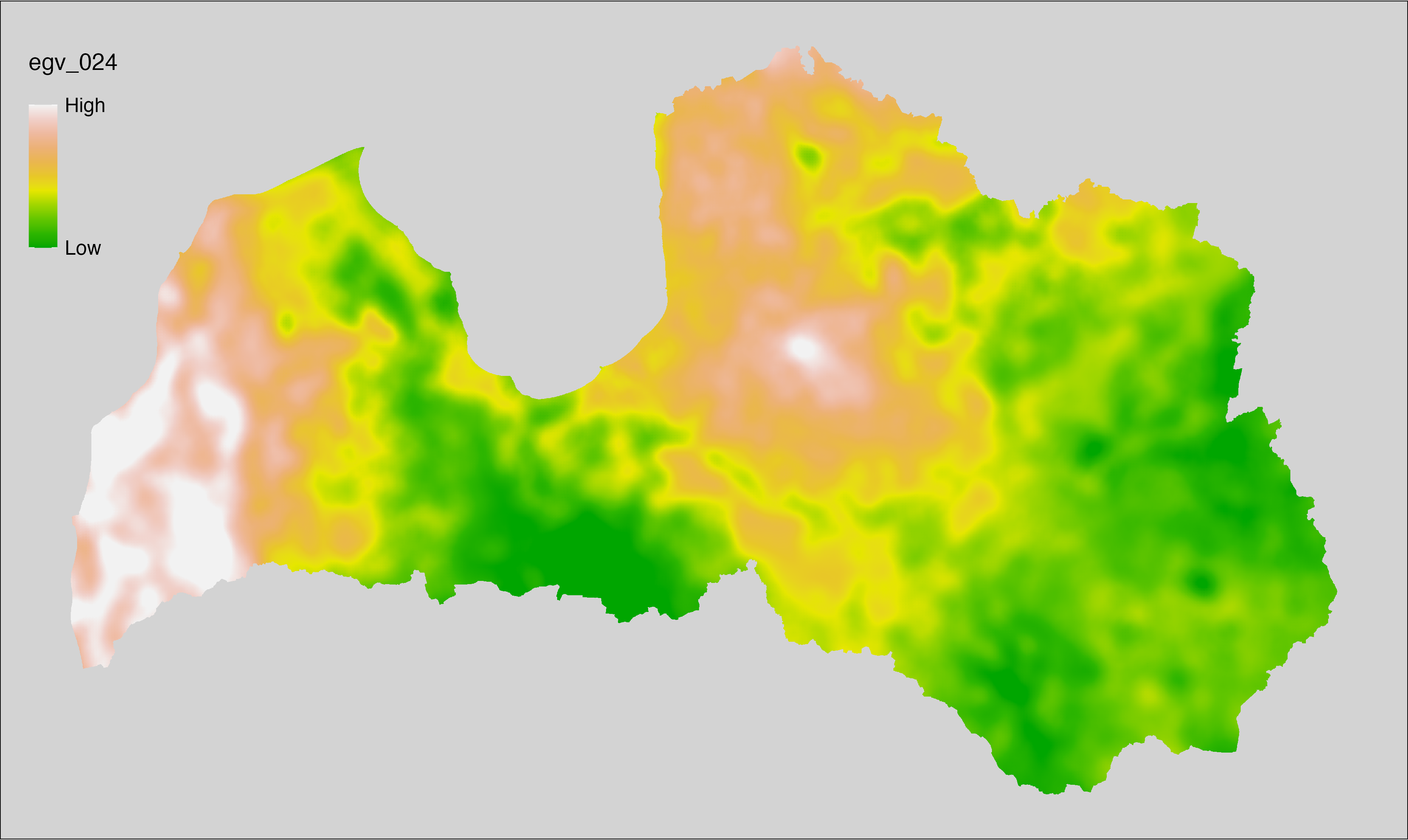
6.25 Climate_CHELSAv2.1-cmi-mean_cell
filename: Climate_CHELSAv2.1-cmi-mean_cell.tif
layername: egv_025
English name: Mean of monthly mean climate moisture index (kg m⁻² month⁻¹) (CHELSA v2.1) within the analysis cell (1 ha)
Latvian name: Vidējais ik mēneša vidējais klimata mitruma indekss (kg m⁻² month⁻¹) (CHELSA v2.1) analīzes šūnā (1 ha)
Procedure: Directly follows CHELSA v2.1. EGV is prepared using
the workflow egvtools::downscale2egv() with inverse distance weighted (power =
2) gap filling and soft smoothing (power = 0.5) over 5 km radius around each cell.
Finally, the layer is standardised by subtracting the arithmetic mean and
dividing by the root mean squared error.
Code
# libs ----
if(!require(egvtools)) {remotes::install_github("aavotins/egvtools"); require(egvtools)}
# job ----
localname="Climate_CHELSAv2.1-cmi-mean_cell.tif"
layername="egv_025"
reading="./Geodata/2024/CHELSA/Climate_CHELSAv2.1-cmi-mean_cell.tif"
df <- downscale2egv(
template_path = "./Templates/TemplateRasters/LV100m_10km.tif",
grid_path = "./Templates/TemplateGrids/tikls1km_sauzeme.parquet",
rawfile_path = reading,
out_path = "./RasterGrids_100m/2024/RAW/",
file_name = localname,
layer_name = layername,
fill_gaps = TRUE,
smooth = TRUE,
smooth_radius_km = 5,
plot_result = TRUE)
print(df)
# standardisation ----
if(!require(terra)) {install.packages("terra"); require(terra)}
if(!require(tidyverse)) {install.packages("tidyverse"); require(tidyverse)}
nosaukums="Climate_CHELSAv2.1-cmi-mean_cell.tif"
ielasisanas_cels=paste0("./RasterGrids_100m/2024/RAW/",nosaukums)
saglabasanas_cels=paste0("./RasterGrids_100m/2024/Scaled/",nosaukums)
slanis=rast(ielasisanas_cels)
videjais=global(slanis,fun="mean",na.rm=TRUE)
centrets=slanis-videjais[,1]
standartnovirze=terra::global(centrets,fun="rms",na.rm=TRUE)
merogots=centrets/standartnovirze[,1]
writeRaster(merogots,
filename=saglabasanas_cels,
overwrite=TRUE)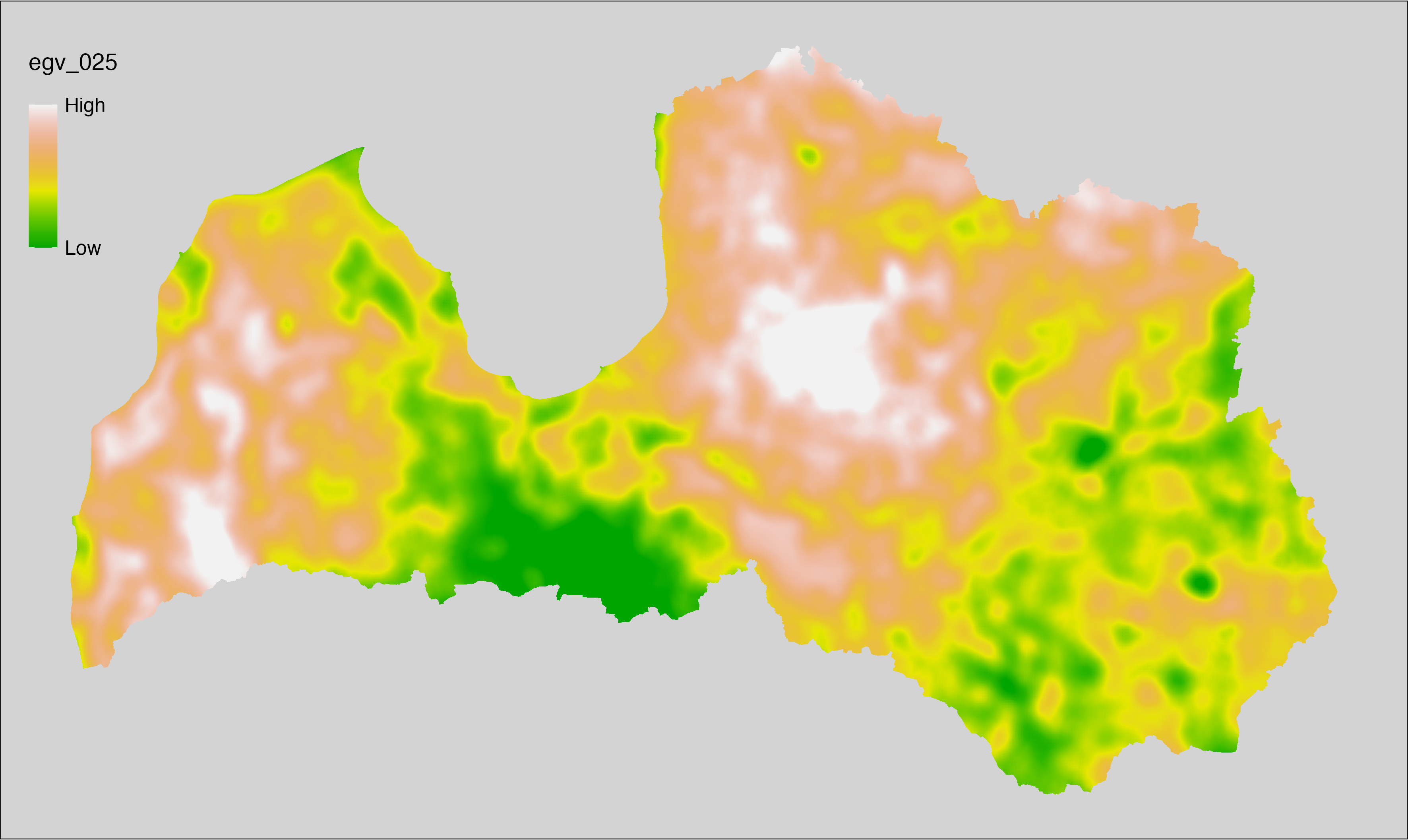
6.26 Climate_CHELSAv2.1-cmi-min_cell
filename: Climate_CHELSAv2.1-cmi-min_cell.tif
layername: egv_026
English name: Mean of monthly minimum climate moisture index (kg m⁻² month⁻¹) (CHELSA v2.1) within the analysis cell (1 ha)
Latvian name: Vidējais ik mēneša minimālais klimata mitruma indekss (kg m⁻² month⁻¹) (CHELSA v2.1) analīzes šūnā (1 ha)
Procedure: Directly follows CHELSA v2.1. EGV is prepared using
the workflow egvtools::downscale2egv() with inverse distance weighted (power =
2) gap filling and soft smoothing (power = 0.5) over 5 km radius around each cell.
Finally, the layer is standardised by subtracting the arithmetic mean and
dividing by the root mean squared error.
Code
# libs ----
if(!require(egvtools)) {remotes::install_github("aavotins/egvtools"); require(egvtools)}
# job ----
localname="Climate_CHELSAv2.1-cmi-min_cell.tif"
layername="egv_026"
reading="./Geodata/2024/CHELSA/Climate_CHELSAv2.1-cmi-min_cell.tif"
df <- downscale2egv(
template_path = "./Templates/TemplateRasters/LV100m_10km.tif",
grid_path = "./Templates/TemplateGrids/tikls1km_sauzeme.parquet",
rawfile_path = reading,
out_path = "./RasterGrids_100m/2024/RAW/",
file_name = localname,
layer_name = layername,
fill_gaps = TRUE,
smooth = TRUE,
smooth_radius_km = 5,
plot_result = TRUE)
print(df)
# standardisation ----
if(!require(terra)) {install.packages("terra"); require(terra)}
if(!require(tidyverse)) {install.packages("tidyverse"); require(tidyverse)}
nosaukums="Climate_CHELSAv2.1-cmi-min_cell.tif"
ielasisanas_cels=paste0("./RasterGrids_100m/2024/RAW/",nosaukums)
saglabasanas_cels=paste0("./RasterGrids_100m/2024/Scaled/",nosaukums)
slanis=rast(ielasisanas_cels)
videjais=global(slanis,fun="mean",na.rm=TRUE)
centrets=slanis-videjais[,1]
standartnovirze=terra::global(centrets,fun="rms",na.rm=TRUE)
merogots=centrets/standartnovirze[,1]
writeRaster(merogots,
filename=saglabasanas_cels,
overwrite=TRUE)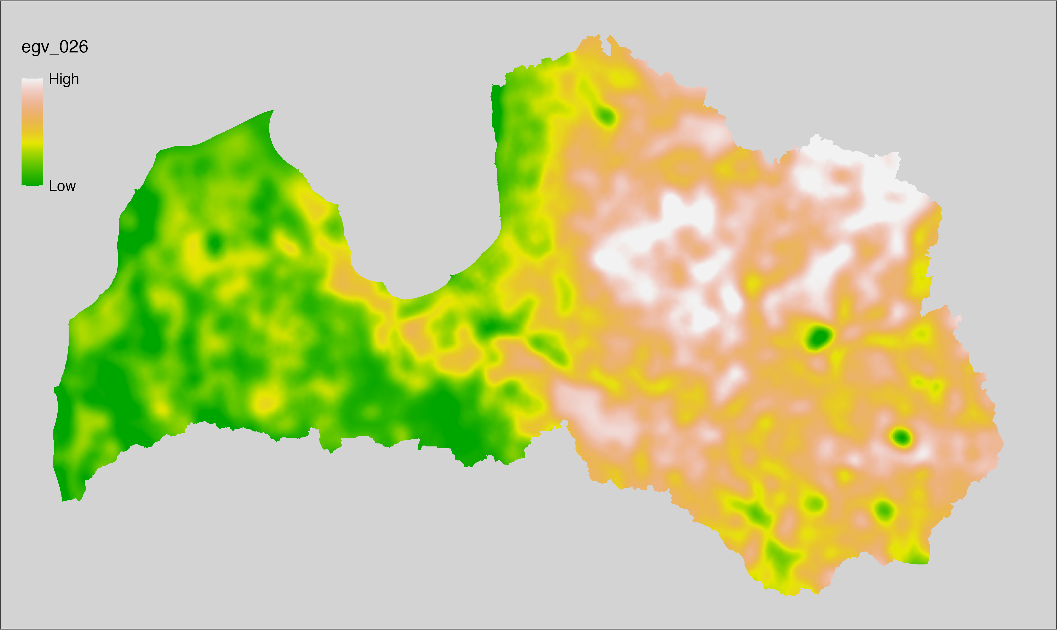
6.27 Climate_CHELSAv2.1-cmi-range_cell
filename: Climate_CHELSAv2.1-cmi-range_cell.tif
layername: egv_027
English name: Annual range of monthly climate moisture index (kg m⁻² month⁻¹) (CHELSA v2.1) within the analysis cell (1 ha)
Latvian name: Gada klimata mitruma indeksa amplitūda (kg m⁻² month⁻¹) (CHELSA v2.1) analīzes šūnā (1 ha)
Procedure: Directly follows CHELSA v2.1. EGV is prepared using
the workflow egvtools::downscale2egv() with inverse distance weighted (power =
2) gap filling and soft smoothing (power = 0.5) over 5 km radius around each cell.
Finally, the layer is standardised by subtracting the arithmetic mean and
dividing by the root mean squared error.
Code
# libs ----
if(!require(egvtools)) {remotes::install_github("aavotins/egvtools"); require(egvtools)}
# job ----
localname="Climate_CHELSAv2.1-cmi-range_cell.tif"
layername="egv_027"
reading="./Geodata/2024/CHELSA/Climate_CHELSAv2.1-cmi-range_cell.tif"
df <- downscale2egv(
template_path = "./Templates/TemplateRasters/LV100m_10km.tif",
grid_path = "./Templates/TemplateGrids/tikls1km_sauzeme.parquet",
rawfile_path = reading,
out_path = "./RasterGrids_100m/2024/RAW/",
file_name = localname,
layer_name = layername,
fill_gaps = TRUE,
smooth = TRUE,
smooth_radius_km = 5,
plot_result = TRUE)
print(df)
# standardisation ----
if(!require(terra)) {install.packages("terra"); require(terra)}
if(!require(tidyverse)) {install.packages("tidyverse"); require(tidyverse)}
nosaukums="Climate_CHELSAv2.1-cmi-range_cell.tif"
ielasisanas_cels=paste0("./RasterGrids_100m/2024/RAW/",nosaukums)
saglabasanas_cels=paste0("./RasterGrids_100m/2024/Scaled/",nosaukums)
slanis=rast(ielasisanas_cels)
videjais=global(slanis,fun="mean",na.rm=TRUE)
centrets=slanis-videjais[,1]
standartnovirze=terra::global(centrets,fun="rms",na.rm=TRUE)
merogots=centrets/standartnovirze[,1]
writeRaster(merogots,
filename=saglabasanas_cels,
overwrite=TRUE)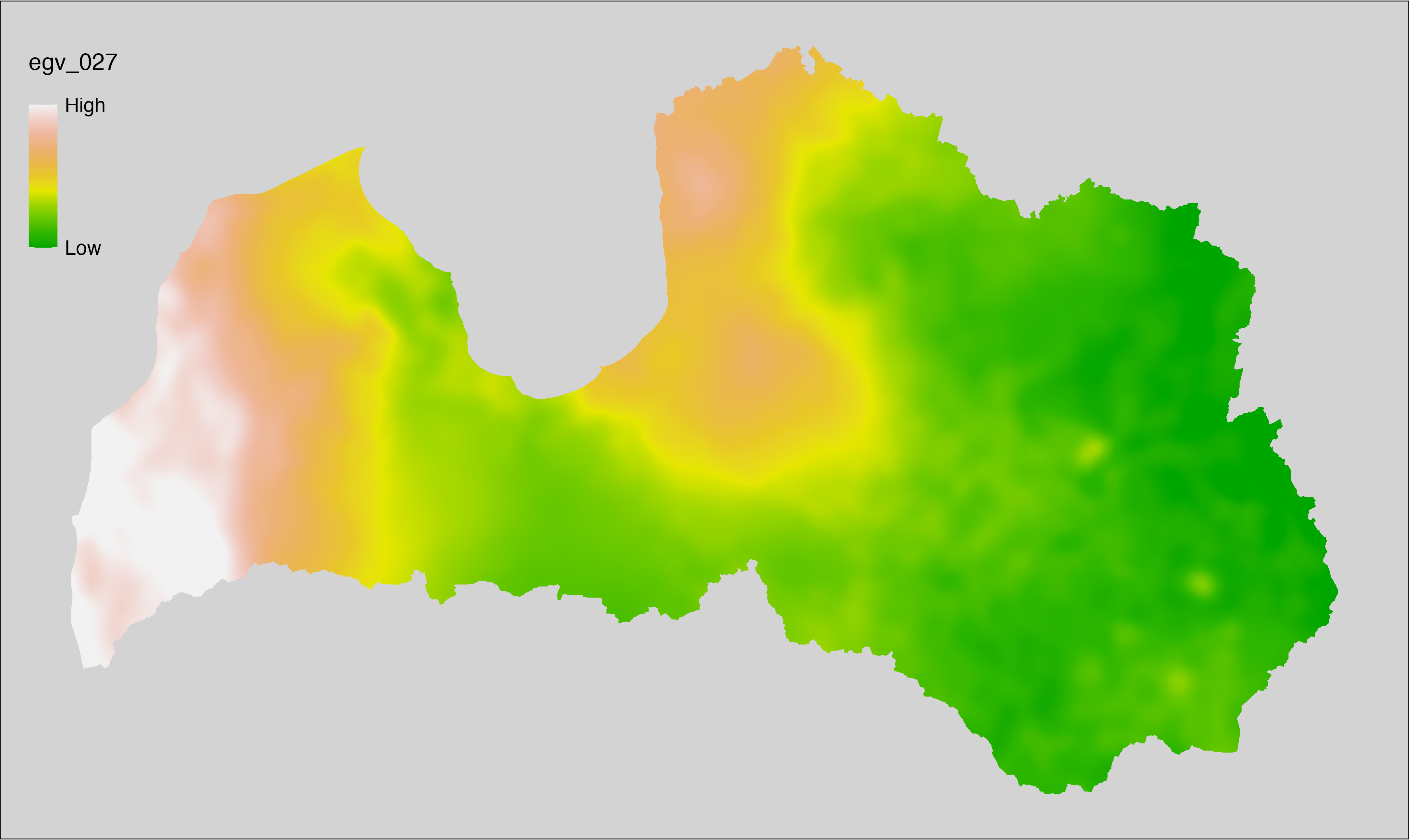
6.28 Climate_CHELSAv2.1-fcf_cell
filename: Climate_CHELSAv2.1-fcf_cell.tif
layername: egv_028
English name: Frost change frequency (number of events in which tmin or tmax go above or below 0°C) (CHELSA v2.1) within the analysis cell (1 ha)
Latvian name: Sasalšanas gadījumu biežums (zemākā vai augstākā temperatūra šķērso 0°C) (CHELSA v2.1) analīzes šūnā (1 ha)
Procedure: Directly follows CHELSA v2.1. EGV is prepared using
the workflow egvtools::downscale2egv() with inverse distance weighted (power =
2) gap filling and soft smoothing (power = 0.5) over 5 km radius around each cell.
Finally, the layer is standardised by subtracting the arithmetic mean and
dividing by the root mean squared error.
Code
# libs ----
if(!require(egvtools)) {remotes::install_github("aavotins/egvtools"); require(egvtools)}
# job ----
localname="Climate_CHELSAv2.1-fcf_cell.tif"
layername="egv_028"
reading="./Geodata/2024/CHELSA/Climate_CHELSAv2.1-fcf_cell.tif"
df <- downscale2egv(
template_path = "./Templates/TemplateRasters/LV100m_10km.tif",
grid_path = "./Templates/TemplateGrids/tikls1km_sauzeme.parquet",
rawfile_path = reading,
out_path = "./RasterGrids_100m/2024/RAW/",
file_name = localname,
layer_name = layername,
fill_gaps = TRUE,
smooth = TRUE,
smooth_radius_km = 5,
plot_result = TRUE)
print(df)
# standardisation ----
if(!require(terra)) {install.packages("terra"); require(terra)}
if(!require(tidyverse)) {install.packages("tidyverse"); require(tidyverse)}
nosaukums="Climate_CHELSAv2.1-fcf_cell.tif"
ielasisanas_cels=paste0("./RasterGrids_100m/2024/RAW/",nosaukums)
saglabasanas_cels=paste0("./RasterGrids_100m/2024/Scaled/",nosaukums)
slanis=rast(ielasisanas_cels)
videjais=global(slanis,fun="mean",na.rm=TRUE)
centrets=slanis-videjais[,1]
standartnovirze=terra::global(centrets,fun="rms",na.rm=TRUE)
merogots=centrets/standartnovirze[,1]
writeRaster(merogots,
filename=saglabasanas_cels,
overwrite=TRUE)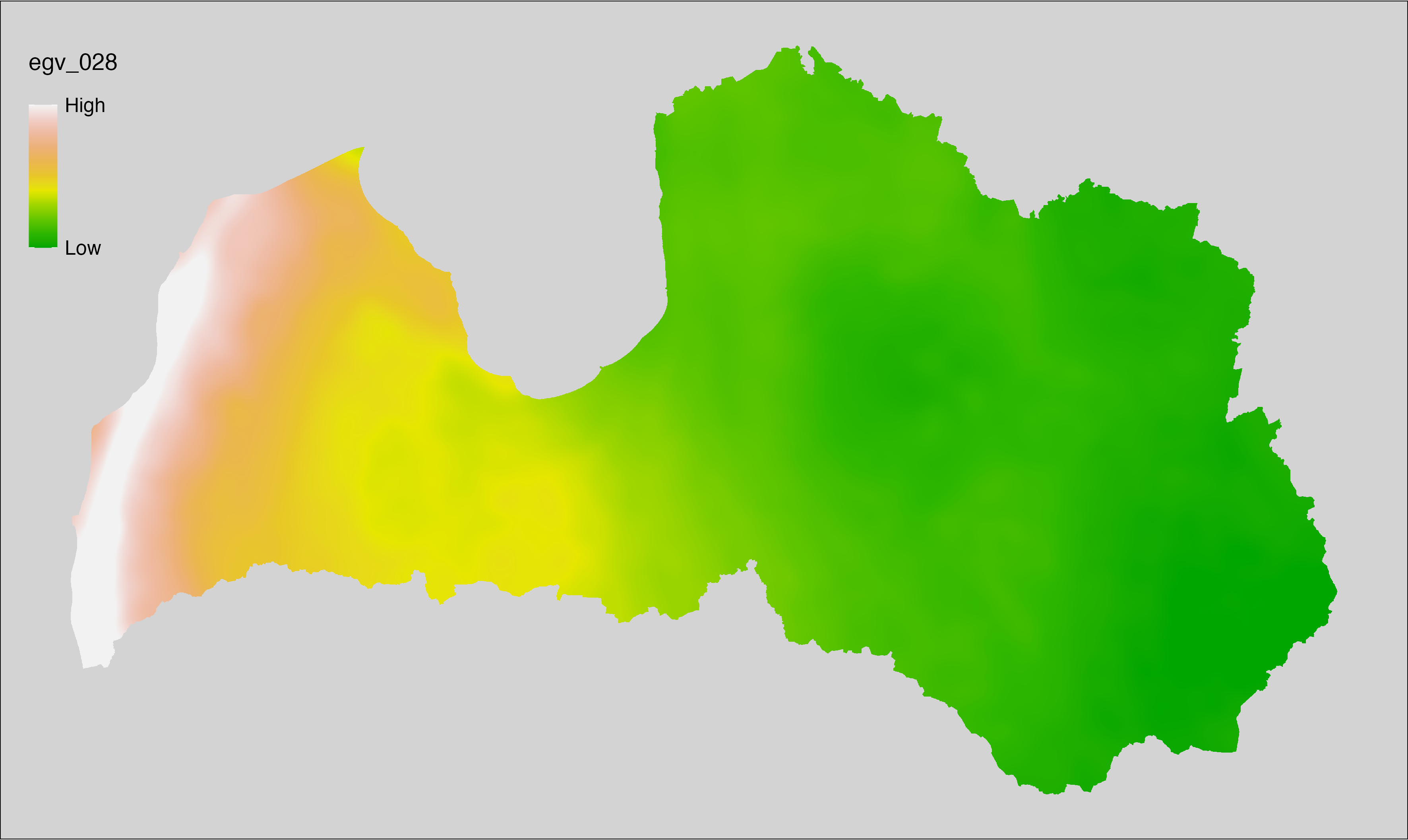
6.29 Climate_CHELSAv2.1-fgd_cell
filename: Climate_CHELSAv2.1-fgd_cell.tif
layername: egv_029
English name: First day of the growing season (TREELIM) (CHELSA v2.1) within the analysis cell (1 ha)
Latvian name: Veģetācijas sezonas pirmā diena (TREELIM) (CHELSA v2.1) analīzes šūnā (1 ha)
Procedure: Directly follows CHELSA v2.1. EGV is prepared using
the workflow egvtools::downscale2egv() with inverse distance weighted (power =
2) gap filling and soft smoothing (power = 0.5) over 5 km radius around each cell.
Finally, the layer is standardised by subtracting the arithmetic mean and
dividing by the root mean squared error.
Code
# libs ----
if(!require(egvtools)) {remotes::install_github("aavotins/egvtools"); require(egvtools)}
# job ----
localname="Climate_CHELSAv2.1-fgd_cell.tif"
layername="egv_029"
reading="./Geodata/2024/CHELSA/Climate_CHELSAv2.1-fgd_cell.tif"
df <- downscale2egv(
template_path = "./Templates/TemplateRasters/LV100m_10km.tif",
grid_path = "./Templates/TemplateGrids/tikls1km_sauzeme.parquet",
rawfile_path = reading,
out_path = "./RasterGrids_100m/2024/RAW/",
file_name = localname,
layer_name = layername,
fill_gaps = TRUE,
smooth = TRUE,
smooth_radius_km = 5,
plot_result = TRUE)
print(df)
# standardisation ----
if(!require(terra)) {install.packages("terra"); require(terra)}
if(!require(tidyverse)) {install.packages("tidyverse"); require(tidyverse)}
nosaukums="Climate_CHELSAv2.1-fgd_cell.tif"
ielasisanas_cels=paste0("./RasterGrids_100m/2024/RAW/",nosaukums)
saglabasanas_cels=paste0("./RasterGrids_100m/2024/Scaled/",nosaukums)
slanis=rast(ielasisanas_cels)
videjais=global(slanis,fun="mean",na.rm=TRUE)
centrets=slanis-videjais[,1]
standartnovirze=terra::global(centrets,fun="rms",na.rm=TRUE)
merogots=centrets/standartnovirze[,1]
writeRaster(merogots,
filename=saglabasanas_cels,
overwrite=TRUE)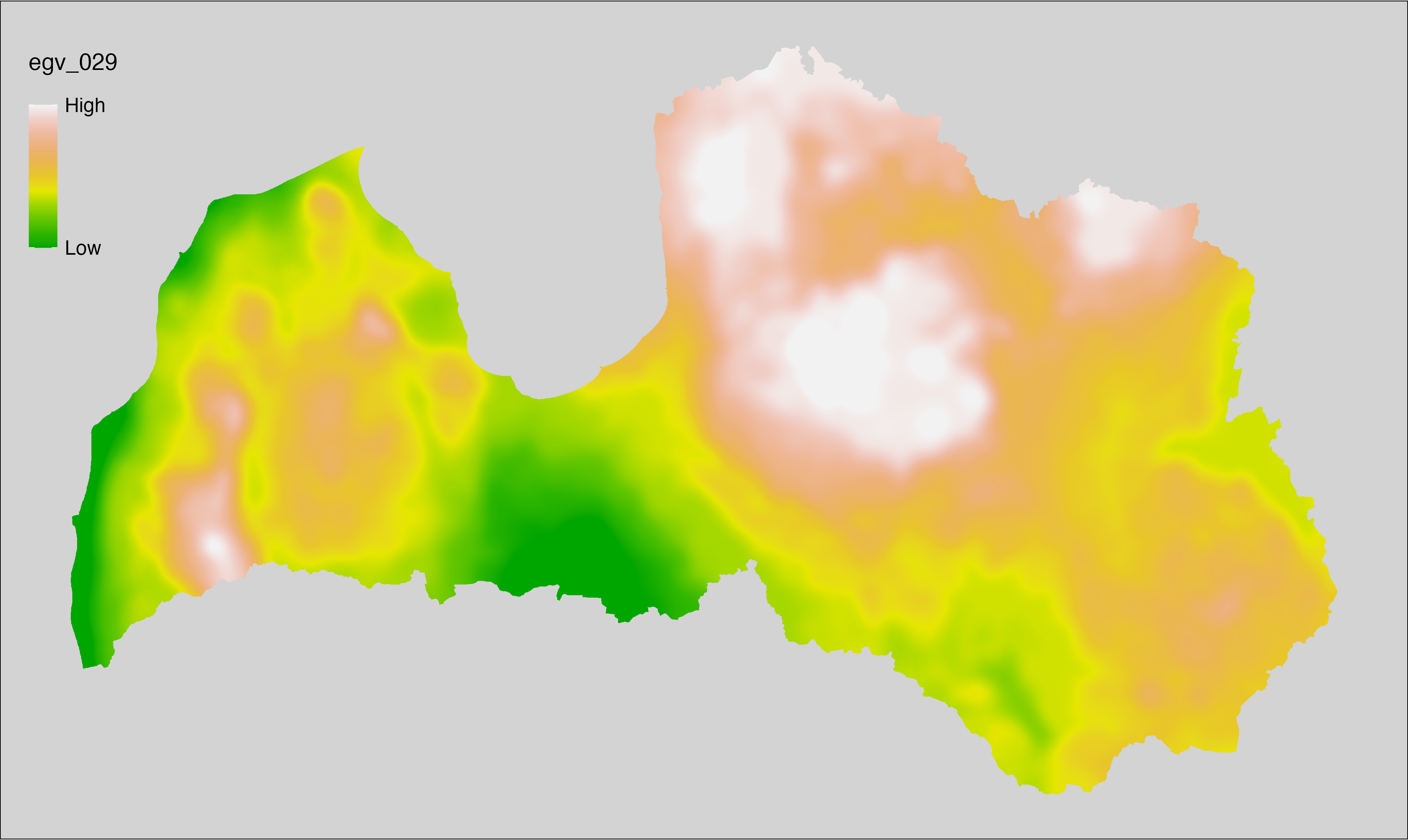
6.30 Climate_CHELSAv2.1-gdd0_cell
filename: Climate_CHELSAv2.1-gdd0_cell.tif
layername: egv_030
English name: Growing degree days temerature sum above 0°C (CHELSA v2.1) within the analysis cell (1 ha)
Latvian name: Aktīvo temperatūru summa no 0°C (CHELSA v2.1) analīzes šūnā (1 ha)
Procedure: Directly follows CHELSA v2.1. EGV is prepared using
the workflow egvtools::downscale2egv() with inverse distance weighted (power =
2) gap filling and soft smoothing (power = 0.5) over 5 km radius around each cell.
Finally, the layer is standardised by subtracting the arithmetic mean and
dividing by the root mean squared error.
Code
# libs ----
if(!require(egvtools)) {remotes::install_github("aavotins/egvtools"); require(egvtools)}
# job ----
localname="Climate_CHELSAv2.1-gdd0_cell.tif"
layername="egv_030"
reading="./Geodata/2024/CHELSA/Climate_CHELSAv2.1-gdd0_cell.tif"
df <- downscale2egv(
template_path = "./Templates/TemplateRasters/LV100m_10km.tif",
grid_path = "./Templates/TemplateGrids/tikls1km_sauzeme.parquet",
rawfile_path = reading,
out_path = "./RasterGrids_100m/2024/RAW/",
file_name = localname,
layer_name = layername,
fill_gaps = TRUE,
smooth = TRUE,
smooth_radius_km = 5,
plot_result = TRUE)
print(df)
# standardisation ----
if(!require(terra)) {install.packages("terra"); require(terra)}
if(!require(tidyverse)) {install.packages("tidyverse"); require(tidyverse)}
nosaukums="Climate_CHELSAv2.1-gdd0_cell.tif"
ielasisanas_cels=paste0("./RasterGrids_100m/2024/RAW/",nosaukums)
saglabasanas_cels=paste0("./RasterGrids_100m/2024/Scaled/",nosaukums)
slanis=rast(ielasisanas_cels)
videjais=global(slanis,fun="mean",na.rm=TRUE)
centrets=slanis-videjais[,1]
standartnovirze=terra::global(centrets,fun="rms",na.rm=TRUE)
merogots=centrets/standartnovirze[,1]
writeRaster(merogots,
filename=saglabasanas_cels,
overwrite=TRUE)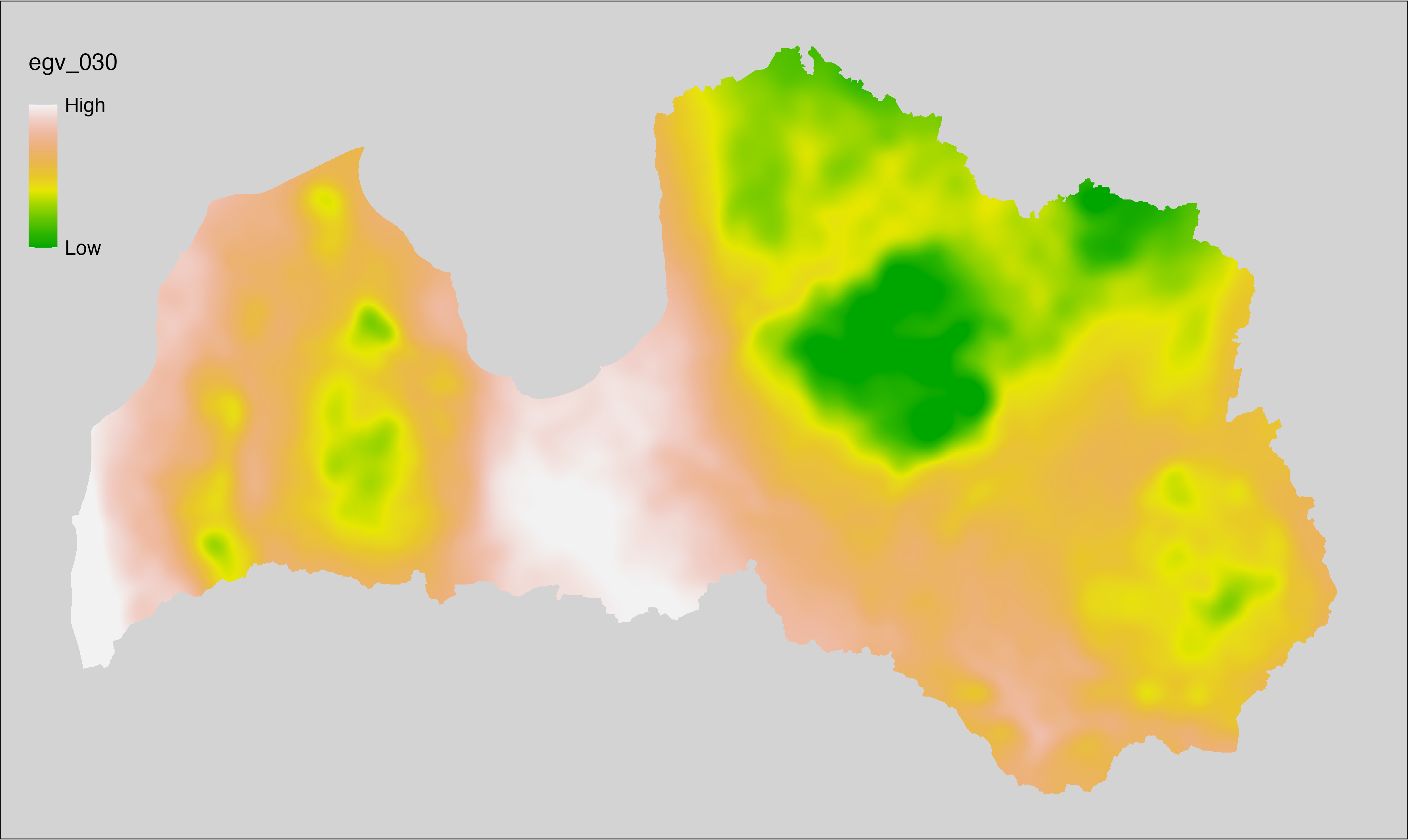
6.31 Climate_CHELSAv2.1-gdd10_cell
filename: Climate_CHELSAv2.1-gdd10_cell.tif
layername: egv_031
English name: Growing degree days temerature sum above 10°C (CHELSA v2.1) within the analysis cell (1 ha)
Latvian name: Aktīvo temperatūru summa no 10°C (CHELSA v2.1) analīzes šūnā (1 ha)
Procedure: Directly follows CHELSA v2.1. EGV is prepared using
the workflow egvtools::downscale2egv() with inverse distance weighted (power =
2) gap filling and soft smoothing (power = 0.5) over 5 km radius around each cell.
Finally, the layer is standardised by subtracting the arithmetic mean and
dividing by the root mean squared error.
Code
# libs ----
if(!require(egvtools)) {remotes::install_github("aavotins/egvtools"); require(egvtools)}
# job ----
localname="Climate_CHELSAv2.1-gdd10_cell.tif"
layername="egv_031"
reading="./Geodata/2024/CHELSA/Climate_CHELSAv2.1-gdd10_cell.tif"
df <- downscale2egv(
template_path = "./Templates/TemplateRasters/LV100m_10km.tif",
grid_path = "./Templates/TemplateGrids/tikls1km_sauzeme.parquet",
rawfile_path = reading,
out_path = "./RasterGrids_100m/2024/RAW/",
file_name = localname,
layer_name = layername,
fill_gaps = TRUE,
smooth = TRUE,
smooth_radius_km = 5,
plot_result = TRUE)
print(df)
# standardisation ----
if(!require(terra)) {install.packages("terra"); require(terra)}
if(!require(tidyverse)) {install.packages("tidyverse"); require(tidyverse)}
nosaukums="Climate_CHELSAv2.1-gdd10_cell.tif"
ielasisanas_cels=paste0("./RasterGrids_100m/2024/RAW/",nosaukums)
saglabasanas_cels=paste0("./RasterGrids_100m/2024/Scaled/",nosaukums)
slanis=rast(ielasisanas_cels)
videjais=global(slanis,fun="mean",na.rm=TRUE)
centrets=slanis-videjais[,1]
standartnovirze=terra::global(centrets,fun="rms",na.rm=TRUE)
merogots=centrets/standartnovirze[,1]
writeRaster(merogots,
filename=saglabasanas_cels,
overwrite=TRUE)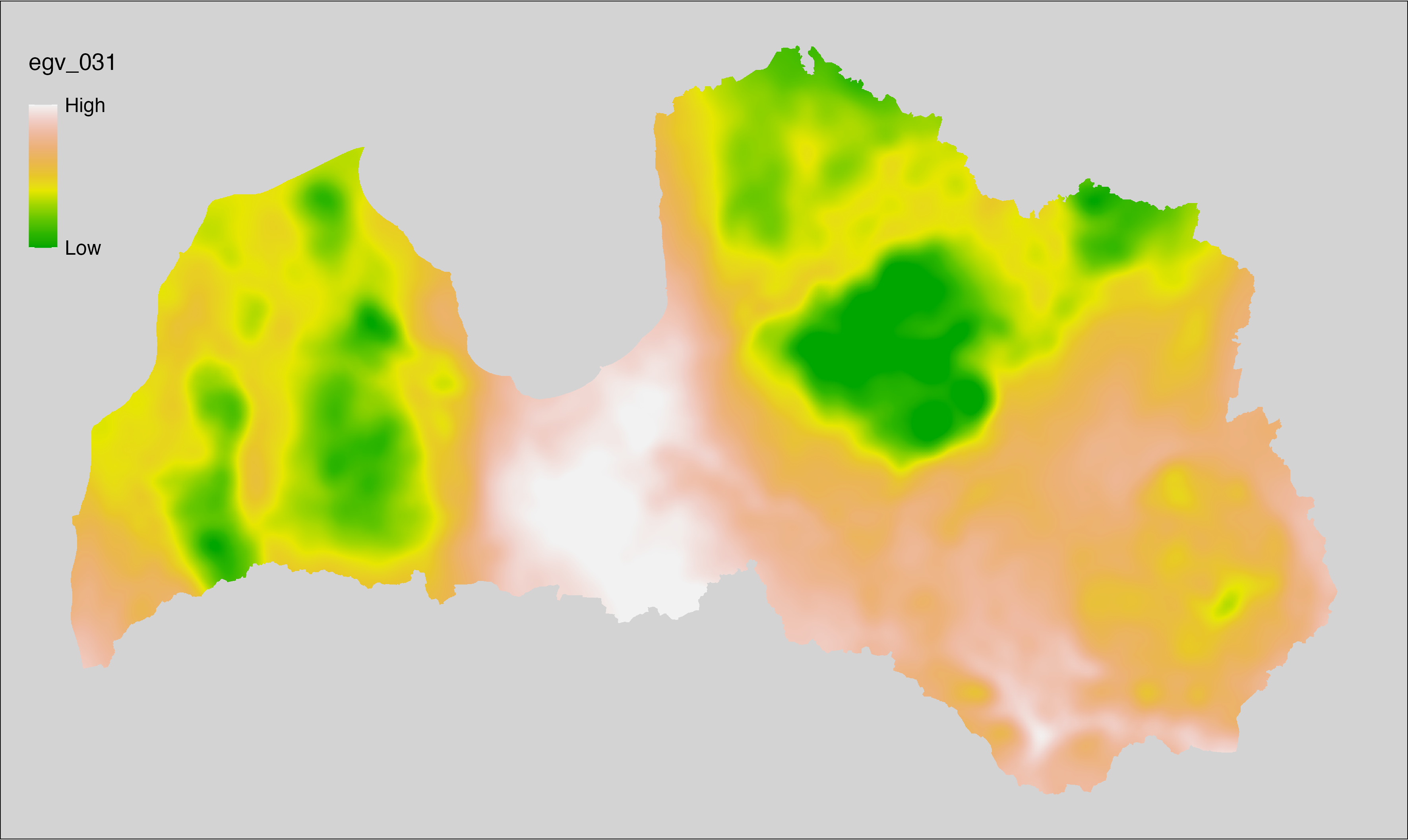
6.32 Climate_CHELSAv2.1-gdd5_cell
filename: Climate_CHELSAv2.1-gdd5_cell.tif
layername: egv_032
English name: Growing degree days temerature sum above 5°C (CHELSA v2.1) within the analysis cell (1 ha)
Latvian name: Aktīvo temperatūru summa no 5°C (CHELSA v2.1) analīzes šūnā (1 ha)
Procedure: Directly follows CHELSA v2.1. EGV is prepared using
the workflow egvtools::downscale2egv() with inverse distance weighted (power =
2) gap filling and soft smoothing (power = 0.5) over 5 km radius around each cell.
Finally, the layer is standardised by subtracting the arithmetic mean and
dividing by the root mean squared error.
Code
# libs ----
if(!require(egvtools)) {remotes::install_github("aavotins/egvtools"); require(egvtools)}
# job ----
localname="Climate_CHELSAv2.1-gdd5_cell.tif"
layername="egv_032"
reading="./Geodata/2024/CHELSA/Climate_CHELSAv2.1-gdd5_cell.tif"
df <- downscale2egv(
template_path = "./Templates/TemplateRasters/LV100m_10km.tif",
grid_path = "./Templates/TemplateGrids/tikls1km_sauzeme.parquet",
rawfile_path = reading,
out_path = "./RasterGrids_100m/2024/RAW/",
file_name = localname,
layer_name = layername,
fill_gaps = TRUE,
smooth = TRUE,
smooth_radius_km = 5,
plot_result = TRUE)
print(df)
# standardisation ----
if(!require(terra)) {install.packages("terra"); require(terra)}
if(!require(tidyverse)) {install.packages("tidyverse"); require(tidyverse)}
nosaukums="Climate_CHELSAv2.1-gdd5_cell.tif"
ielasisanas_cels=paste0("./RasterGrids_100m/2024/RAW/",nosaukums)
saglabasanas_cels=paste0("./RasterGrids_100m/2024/Scaled/",nosaukums)
slanis=rast(ielasisanas_cels)
videjais=global(slanis,fun="mean",na.rm=TRUE)
centrets=slanis-videjais[,1]
standartnovirze=terra::global(centrets,fun="rms",na.rm=TRUE)
merogots=centrets/standartnovirze[,1]
writeRaster(merogots,
filename=saglabasanas_cels,
overwrite=TRUE)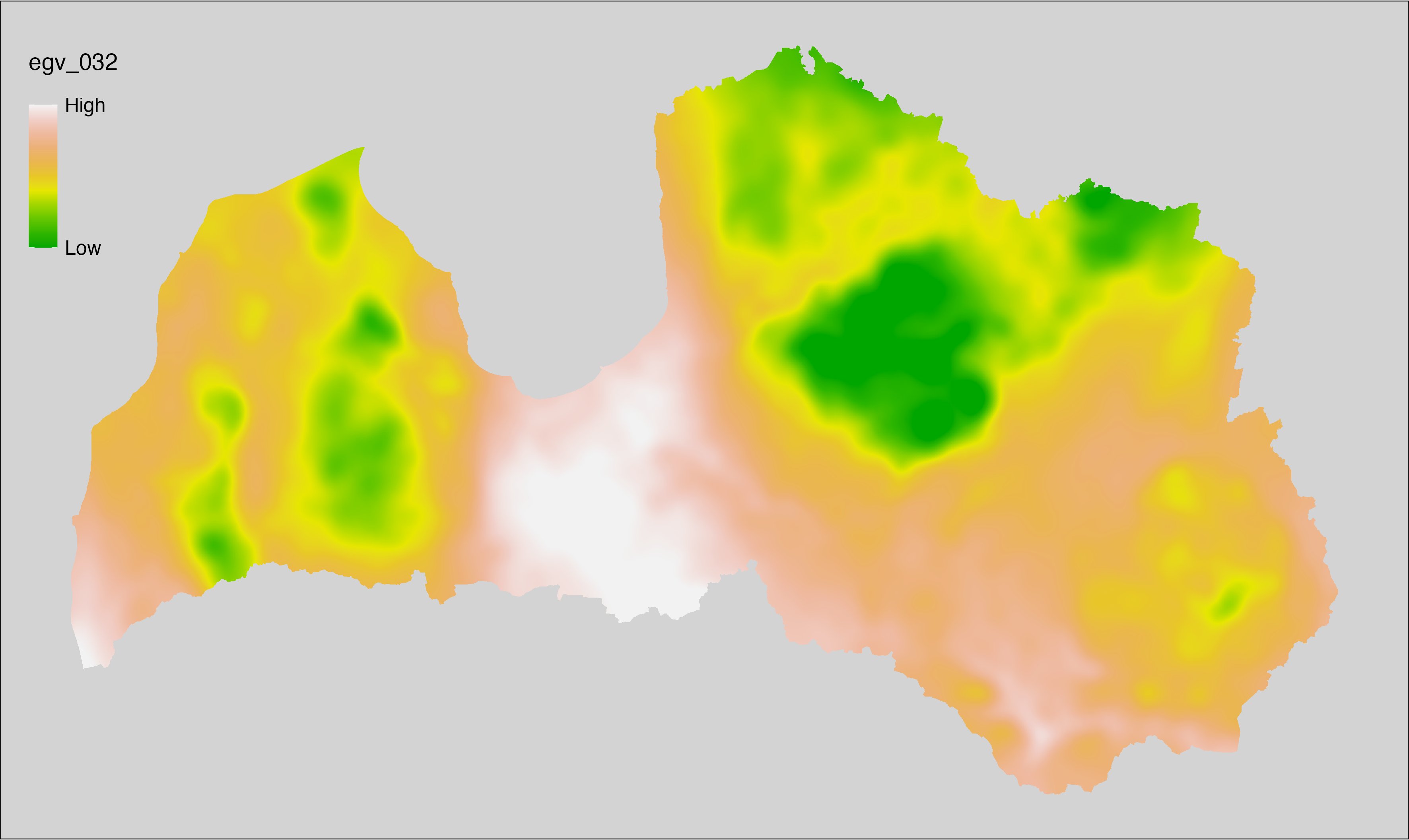
6.33 Climate_CHELSAv2.1-gddlgd0_cell
filename: Climate_CHELSAv2.1-gddlgd0_cell.tif
layername: egv_033
English name: Last growing degree day above 0°C (CHELSA v2.1) within the analysis cell (1 ha)
Latvian name: Veģetācijas sezonas no 0°C pēdējā diena (CHELSA v2.1) analīzes šūnā (1 ha)
Procedure: Directly follows CHELSA v2.1. EGV is prepared using
the workflow egvtools::downscale2egv() with inverse distance weighted (power =
2) gap filling and soft smoothing (power = 0.5) over 5 km radius around each cell.
Finally, the layer is standardised by subtracting the arithmetic mean and
dividing by the root mean squared error.
Code
# libs ----
if(!require(egvtools)) {remotes::install_github("aavotins/egvtools"); require(egvtools)}
# job ----
localname="Climate_CHELSAv2.1-gddlgd0_cell.tif"
layername="egv_033"
reading="./Geodata/2024/CHELSA/Climate_CHELSAv2.1-gddlgd0_cell.tif"
df <- downscale2egv(
template_path = "./Templates/TemplateRasters/LV100m_10km.tif",
grid_path = "./Templates/TemplateGrids/tikls1km_sauzeme.parquet",
rawfile_path = reading,
out_path = "./RasterGrids_100m/2024/RAW/",
file_name = localname,
layer_name = layername,
fill_gaps = TRUE,
smooth = TRUE,
smooth_radius_km = 5,
plot_result = TRUE)
print(df)
# standardisation ----
if(!require(terra)) {install.packages("terra"); require(terra)}
if(!require(tidyverse)) {install.packages("tidyverse"); require(tidyverse)}
nosaukums="Climate_CHELSAv2.1-gddlgd0_cell.tif"
ielasisanas_cels=paste0("./RasterGrids_100m/2024/RAW/",nosaukums)
saglabasanas_cels=paste0("./RasterGrids_100m/2024/Scaled/",nosaukums)
slanis=rast(ielasisanas_cels)
videjais=global(slanis,fun="mean",na.rm=TRUE)
centrets=slanis-videjais[,1]
standartnovirze=terra::global(centrets,fun="rms",na.rm=TRUE)
merogots=centrets/standartnovirze[,1]
writeRaster(merogots,
filename=saglabasanas_cels,
overwrite=TRUE)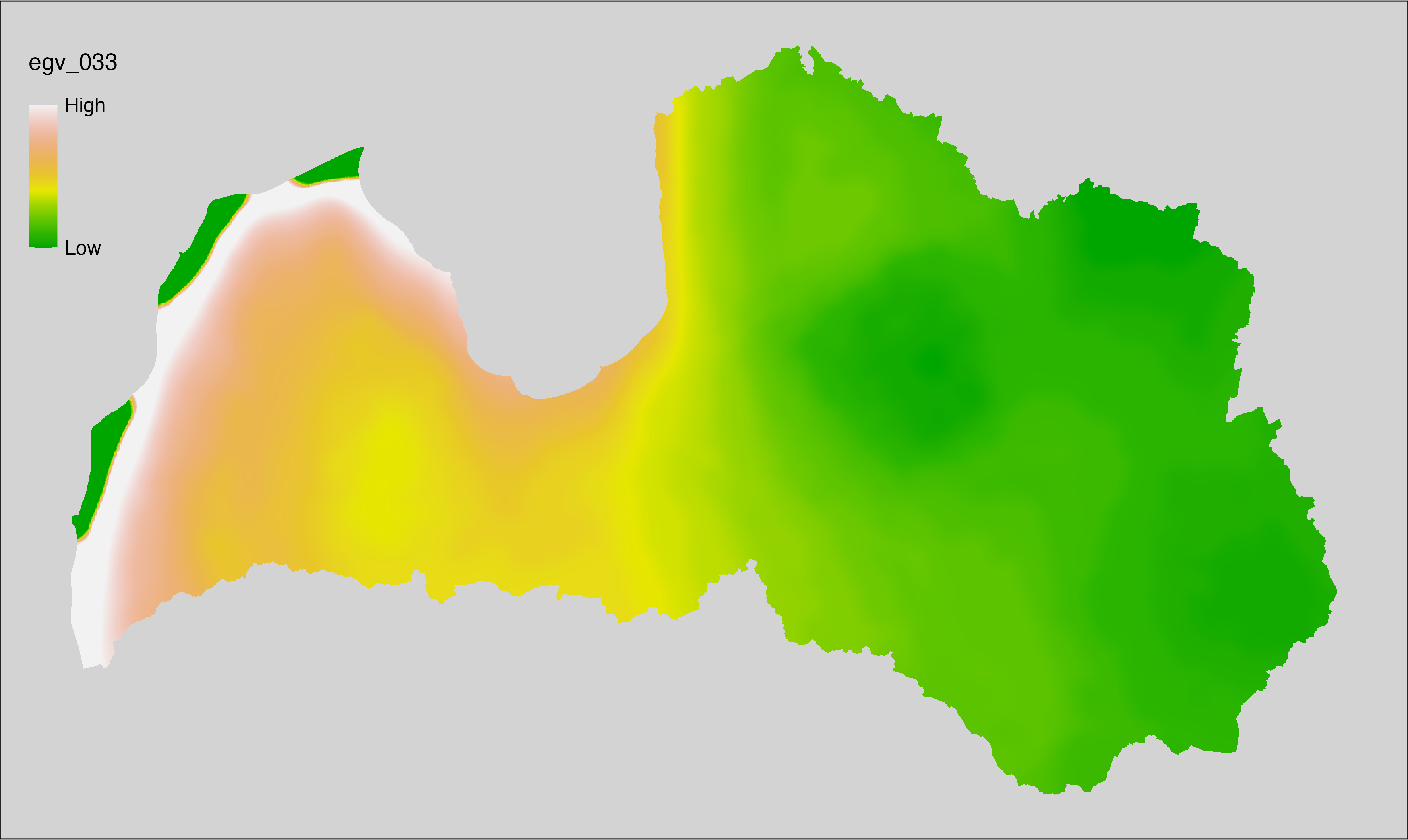
6.34 Climate_CHELSAv2.1-gddlgd10_cell
filename: Climate_CHELSAv2.1-gddlgd10_cell.tif
layername: egv_034
English name: Last growing degree day above 10°C (CHELSA v2.1) within the analysis cell (1 ha)
Latvian name: Veģetācijas sezonas no 10°C pēdējā diena (CHELSA v2.1) analīzes šūnā (1 ha)
Procedure: Directly follows CHELSA v2.1. EGV is prepared using
the workflow egvtools::downscale2egv() with inverse distance weighted (power =
2) gap filling and soft smoothing (power = 0.5) over 5 km radius around each cell.
Finally, the layer is standardised by subtracting the arithmetic mean and
dividing by the root mean squared error.
Code
# libs ----
if(!require(egvtools)) {remotes::install_github("aavotins/egvtools"); require(egvtools)}
# job ----
localname="Climate_CHELSAv2.1-gddlgd10_cell.tif"
layername="egv_034"
reading="./Geodata/2024/CHELSA/Climate_CHELSAv2.1-gddlgd10_cell.tif"
df <- downscale2egv(
template_path = "./Templates/TemplateRasters/LV100m_10km.tif",
grid_path = "./Templates/TemplateGrids/tikls1km_sauzeme.parquet",
rawfile_path = reading,
out_path = "./RasterGrids_100m/2024/RAW/",
file_name = localname,
layer_name = layername,
fill_gaps = TRUE,
smooth = TRUE,
smooth_radius_km = 5,
plot_result = TRUE)
print(df)
# standardisation ----
if(!require(terra)) {install.packages("terra"); require(terra)}
if(!require(tidyverse)) {install.packages("tidyverse"); require(tidyverse)}
nosaukums="Climate_CHELSAv2.1-gddlgd10_cell.tif"
ielasisanas_cels=paste0("./RasterGrids_100m/2024/RAW/",nosaukums)
saglabasanas_cels=paste0("./RasterGrids_100m/2024/Scaled/",nosaukums)
slanis=rast(ielasisanas_cels)
videjais=global(slanis,fun="mean",na.rm=TRUE)
centrets=slanis-videjais[,1]
standartnovirze=terra::global(centrets,fun="rms",na.rm=TRUE)
merogots=centrets/standartnovirze[,1]
writeRaster(merogots,
filename=saglabasanas_cels,
overwrite=TRUE)
6.35 Climate_CHELSAv2.1-gddlgd5_cell
filename: Climate_CHELSAv2.1-gddlgd5_cell.tif
layername: egv_035
English name: Last growing degree day above 5°C (CHELSA v2.1) within the analysis cell (1 ha)
Latvian name: Veģetācijas sezonas no 5°C pēdējā diena (CHELSA v2.1) analīzes šūnā (1 ha)
Procedure: Directly follows CHELSA v2.1. EGV is prepared using
the workflow egvtools::downscale2egv() with inverse distance weighted (power =
2) gap filling and soft smoothing (power = 0.5) over 5 km radius around each cell.
Finally, the layer is standardised by subtracting the arithmetic mean and
dividing by the root mean squared error.
Code
# libs ----
if(!require(egvtools)) {remotes::install_github("aavotins/egvtools"); require(egvtools)}
# job ----
localname="Climate_CHELSAv2.1-gddlgd5_cell.tif"
layername="egv_035"
reading="./Geodata/2024/CHELSA/Climate_CHELSAv2.1-gddlgd5_cell.tif"
df <- downscale2egv(
template_path = "./Templates/TemplateRasters/LV100m_10km.tif",
grid_path = "./Templates/TemplateGrids/tikls1km_sauzeme.parquet",
rawfile_path = reading,
out_path = "./RasterGrids_100m/2024/RAW/",
file_name = localname,
layer_name = layername,
fill_gaps = TRUE,
smooth = TRUE,
smooth_radius_km = 5,
plot_result = TRUE)
print(df)
# standardisation ----
if(!require(terra)) {install.packages("terra"); require(terra)}
if(!require(tidyverse)) {install.packages("tidyverse"); require(tidyverse)}
nosaukums="Climate_CHELSAv2.1-gddlgd5_cell.tif"
ielasisanas_cels=paste0("./RasterGrids_100m/2024/RAW/",nosaukums)
saglabasanas_cels=paste0("./RasterGrids_100m/2024/Scaled/",nosaukums)
slanis=rast(ielasisanas_cels)
videjais=global(slanis,fun="mean",na.rm=TRUE)
centrets=slanis-videjais[,1]
standartnovirze=terra::global(centrets,fun="rms",na.rm=TRUE)
merogots=centrets/standartnovirze[,1]
writeRaster(merogots,
filename=saglabasanas_cels,
overwrite=TRUE)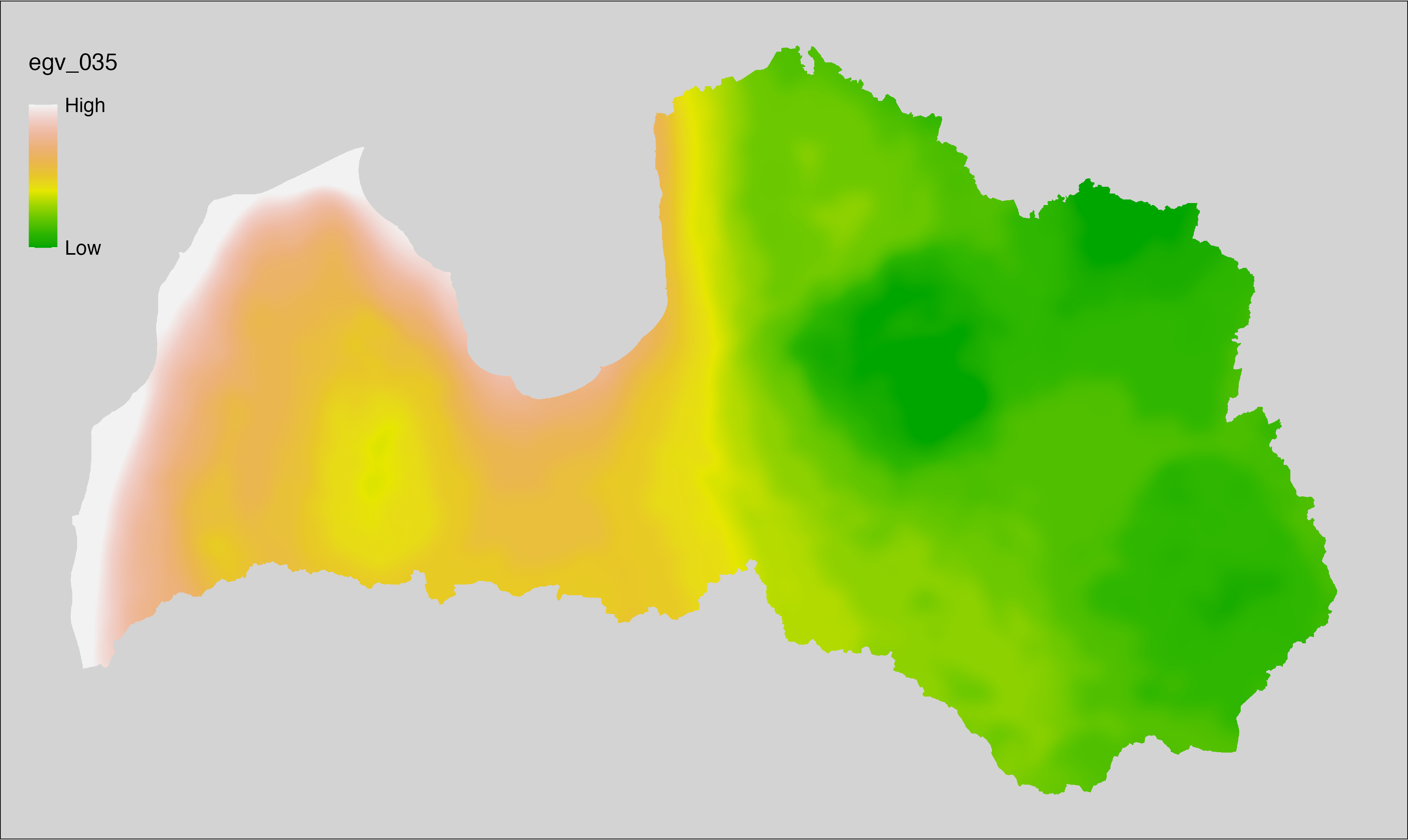
6.36 Climate_CHELSAv2.1-gdgfgd0_cell
filename: Climate_CHELSAv2.1-gdgfgd0_cell.tif
layername: egv_036
English name: First growing degree day above 0°C (CHELSA v2.1) within the analysis cell (1 ha)
Latvian name: Veģetācijas sezonas no 0°C pirmā diena (CHELSA v2.1) analīzes šūnā (1 ha)
Procedure: Directly follows CHELSA v2.1. EGV is prepared using
the workflow egvtools::downscale2egv() with inverse distance weighted (power =
2) gap filling and soft smoothing (power = 0.5) over 5 km radius around each cell.
Finally, the layer is standardised by subtracting the arithmetic mean and
dividing by the root mean squared error.
Code
# libs ----
if(!require(egvtools)) {remotes::install_github("aavotins/egvtools"); require(egvtools)}
# job ----
localname="Climate_CHELSAv2.1-gdgfgd0_cell.tif"
layername="egv_036"
reading="./Geodata/2024/CHELSA/Climate_CHELSAv2.1-gdgfgd0_cell.tif"
df <- downscale2egv(
template_path = "./Templates/TemplateRasters/LV100m_10km.tif",
grid_path = "./Templates/TemplateGrids/tikls1km_sauzeme.parquet",
rawfile_path = reading,
out_path = "./RasterGrids_100m/2024/RAW/",
file_name = localname,
layer_name = layername,
fill_gaps = TRUE,
smooth = TRUE,
smooth_radius_km = 5,
plot_result = TRUE)
print(df)
# standardisation ----
if(!require(terra)) {install.packages("terra"); require(terra)}
if(!require(tidyverse)) {install.packages("tidyverse"); require(tidyverse)}
nosaukums="Climate_CHELSAv2.1-gdgfgd0_cell.tif"
ielasisanas_cels=paste0("./RasterGrids_100m/2024/RAW/",nosaukums)
saglabasanas_cels=paste0("./RasterGrids_100m/2024/Scaled/",nosaukums)
slanis=rast(ielasisanas_cels)
videjais=global(slanis,fun="mean",na.rm=TRUE)
centrets=slanis-videjais[,1]
standartnovirze=terra::global(centrets,fun="rms",na.rm=TRUE)
merogots=centrets/standartnovirze[,1]
writeRaster(merogots,
filename=saglabasanas_cels,
overwrite=TRUE)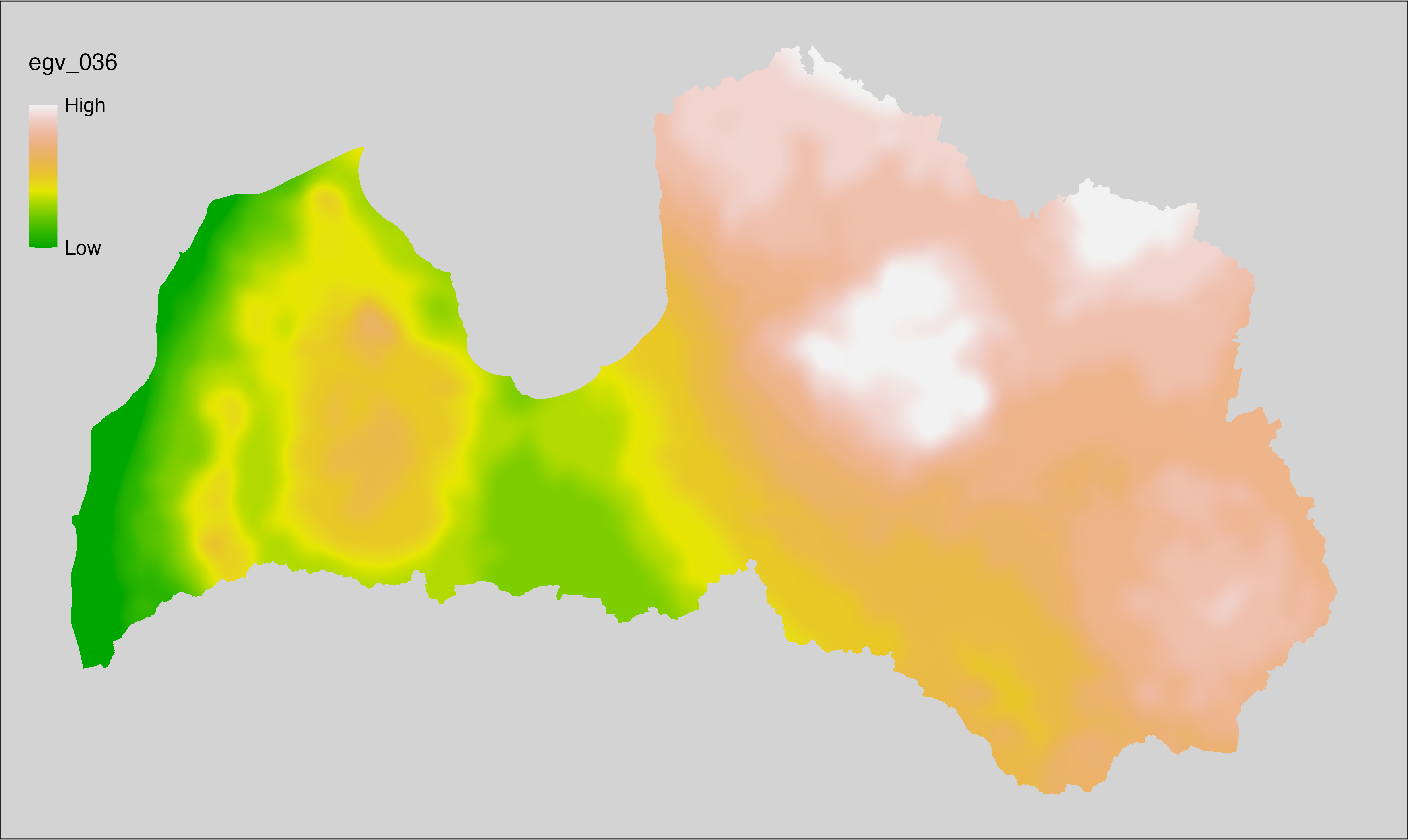
6.37 Climate_CHELSAv2.1-gdgfgd10_cell
filename: Climate_CHELSAv2.1-gdgfgd10_cell.tif
layername: egv_037
English name: First growing degree day above 10°C (CHELSA v2.1) within the analysis cell (1 ha)
Latvian name: Veģetācijas sezonas no 10°C pirmā diena (CHELSA v2.1) analīzes šūnā (1 ha)
Procedure: Directly follows CHELSA v2.1. EGV is prepared using
the workflow egvtools::downscale2egv() with inverse distance weighted (power =
2) gap filling and soft smoothing (power = 0.5) over 5 km radius around each cell.
Finally, the layer is standardised by subtracting the arithmetic mean and
dividing by the root mean squared error.
Code
# libs ----
if(!require(egvtools)) {remotes::install_github("aavotins/egvtools"); require(egvtools)}
# job ----
localname="Climate_CHELSAv2.1-gdgfgd10_cell.tif"
layername="egv_037"
reading="./Geodata/2024/CHELSA/Climate_CHELSAv2.1-gdgfgd10_cell.tif"
df <- downscale2egv(
template_path = "./Templates/TemplateRasters/LV100m_10km.tif",
grid_path = "./Templates/TemplateGrids/tikls1km_sauzeme.parquet",
rawfile_path = reading,
out_path = "./RasterGrids_100m/2024/RAW/",
file_name = localname,
layer_name = layername,
fill_gaps = TRUE,
smooth = TRUE,
smooth_radius_km = 5,
plot_result = TRUE)
print(df)
# standardisation ----
if(!require(terra)) {install.packages("terra"); require(terra)}
if(!require(tidyverse)) {install.packages("tidyverse"); require(tidyverse)}
nosaukums="Climate_CHELSAv2.1-gdgfgd10_cell.tif"
ielasisanas_cels=paste0("./RasterGrids_100m/2024/RAW/",nosaukums)
saglabasanas_cels=paste0("./RasterGrids_100m/2024/Scaled/",nosaukums)
slanis=rast(ielasisanas_cels)
videjais=global(slanis,fun="mean",na.rm=TRUE)
centrets=slanis-videjais[,1]
standartnovirze=terra::global(centrets,fun="rms",na.rm=TRUE)
merogots=centrets/standartnovirze[,1]
writeRaster(merogots,
filename=saglabasanas_cels,
overwrite=TRUE)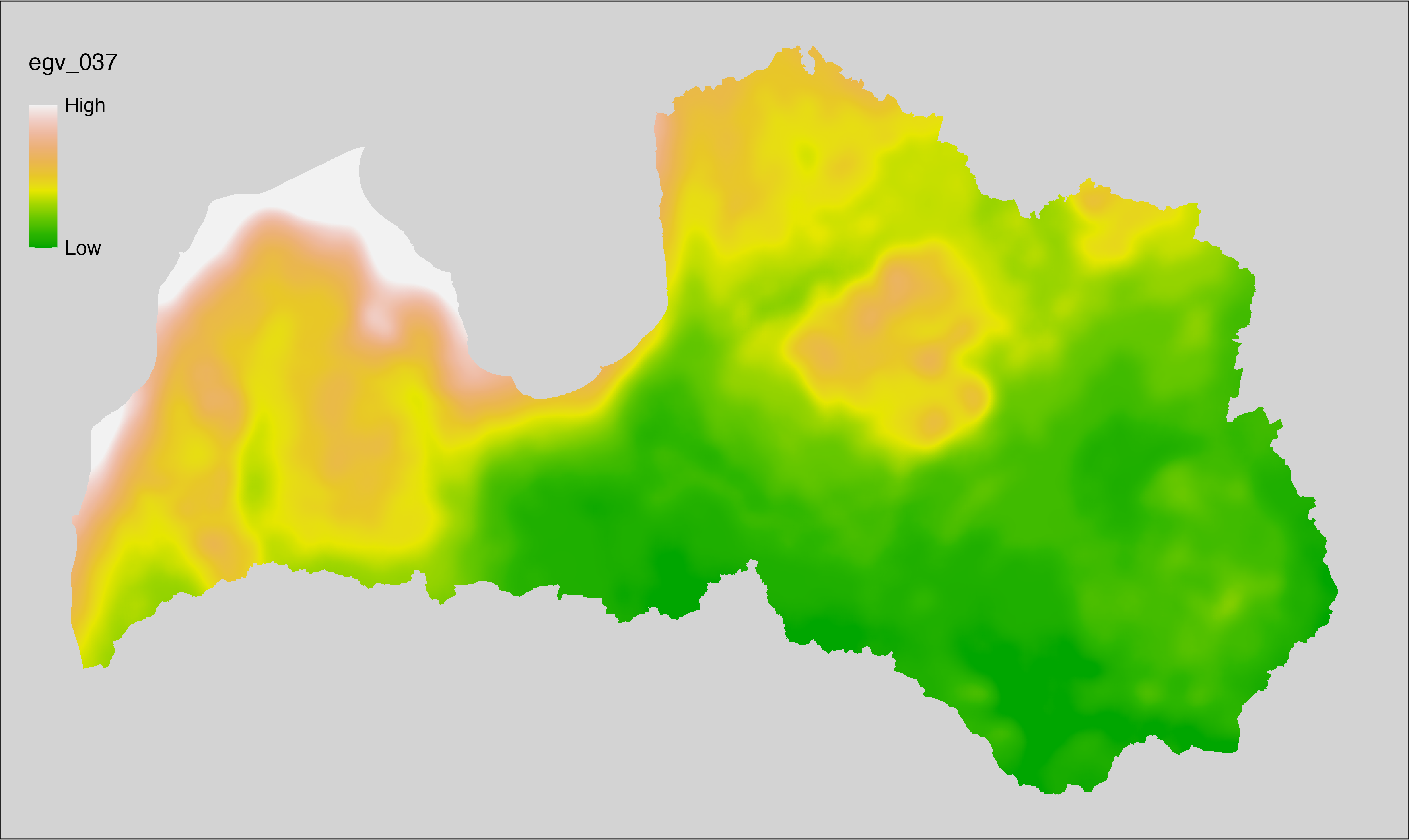
6.38 Climate_CHELSAv2.1-gdgfgd5_cell
filename: Climate_CHELSAv2.1-gdgfgd5_cell.tif
layername: egv_038
English name: First growing degree day above 5°C (CHELSA v2.1) within the analysis cell (1 ha)
Latvian name: Veģetācijas sezonas no 5°C pirmā diena (CHELSA v2.1) analīzes šūnā (1 ha)
Procedure: Directly follows CHELSA v2.1. EGV is prepared using
the workflow egvtools::downscale2egv() with inverse distance weighted (power =
2) gap filling and soft smoothing (power = 0.5) over 5 km radius around each cell.
Finally, the layer is standardised by subtracting the arithmetic mean and
dividing by the root mean squared error.
Code
# libs ----
if(!require(egvtools)) {remotes::install_github("aavotins/egvtools"); require(egvtools)}
# job ----
localname="Climate_CHELSAv2.1-gdgfgd5_cell.tif"
layername="egv_038"
reading="./Geodata/2024/CHELSA/Climate_CHELSAv2.1-gdgfgd5_cell.tif"
df <- downscale2egv(
template_path = "./Templates/TemplateRasters/LV100m_10km.tif",
grid_path = "./Templates/TemplateGrids/tikls1km_sauzeme.parquet",
rawfile_path = reading,
out_path = "./RasterGrids_100m/2024/RAW/",
file_name = localname,
layer_name = layername,
fill_gaps = TRUE,
smooth = TRUE,
smooth_radius_km = 5,
plot_result = TRUE)
print(df)
# standardisation ----
if(!require(terra)) {install.packages("terra"); require(terra)}
if(!require(tidyverse)) {install.packages("tidyverse"); require(tidyverse)}
nosaukums="Climate_CHELSAv2.1-gdgfgd5_cell.tif"
ielasisanas_cels=paste0("./RasterGrids_100m/2024/RAW/",nosaukums)
saglabasanas_cels=paste0("./RasterGrids_100m/2024/Scaled/",nosaukums)
slanis=rast(ielasisanas_cels)
videjais=global(slanis,fun="mean",na.rm=TRUE)
centrets=slanis-videjais[,1]
standartnovirze=terra::global(centrets,fun="rms",na.rm=TRUE)
merogots=centrets/standartnovirze[,1]
writeRaster(merogots,
filename=saglabasanas_cels,
overwrite=TRUE)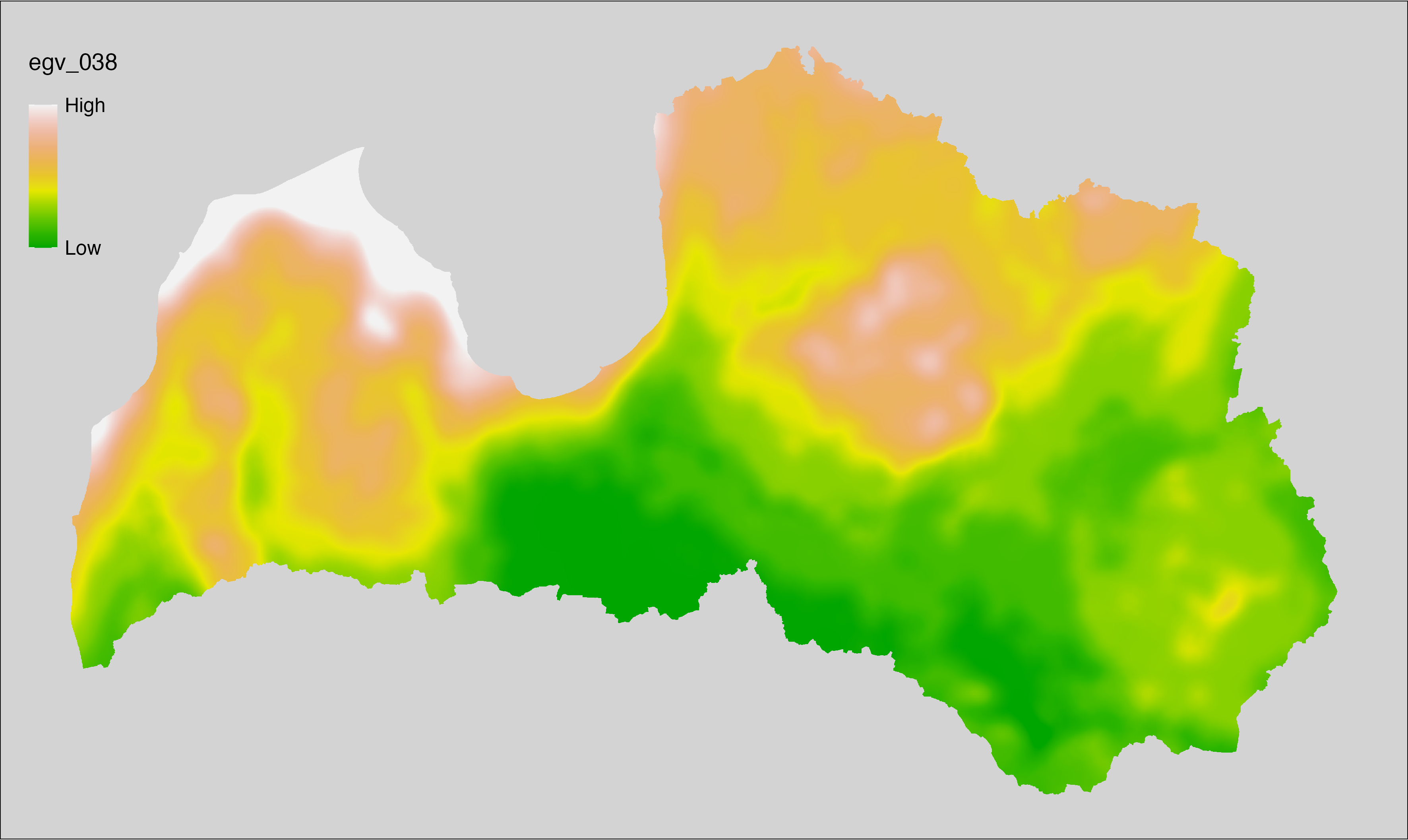
6.39 Climate_CHELSAv2.1-gsl_cell
filename: Climate_CHELSAv2.1-gsl_cell.tif
layername: egv_039
English name: Length of the growing season (TREELIM) (CHELSA v2.1) within the analysis cell (1 ha)
Latvian name: Veģetācijas sezonas garums (TREELIM) (CHELSA v2.1) analīzes šūnā (1 ha)
Procedure: Directly follows CHELSA v2.1. EGV is prepared using
the workflow egvtools::downscale2egv() with inverse distance weighted (power =
2) gap filling and soft smoothing (power = 0.5) over 5 km radius around each cell.
Finally, the layer is standardised by subtracting the arithmetic mean and
dividing by the root mean squared error.
Code
# libs ----
if(!require(egvtools)) {remotes::install_github("aavotins/egvtools"); require(egvtools)}
# job ----
localname="Climate_CHELSAv2.1-gsl_cell.tif"
layername="egv_039"
reading="./Geodata/2024/CHELSA/Climate_CHELSAv2.1-gsl_cell.tif"
df <- downscale2egv(
template_path = "./Templates/TemplateRasters/LV100m_10km.tif",
grid_path = "./Templates/TemplateGrids/tikls1km_sauzeme.parquet",
rawfile_path = reading,
out_path = "./RasterGrids_100m/2024/RAW/",
file_name = localname,
layer_name = layername,
fill_gaps = TRUE,
smooth = TRUE,
smooth_radius_km = 5,
plot_result = TRUE)
print(df)
# standardisation ----
if(!require(terra)) {install.packages("terra"); require(terra)}
if(!require(tidyverse)) {install.packages("tidyverse"); require(tidyverse)}
nosaukums="Climate_CHELSAv2.1-gsl_cell.tif"
ielasisanas_cels=paste0("./RasterGrids_100m/2024/RAW/",nosaukums)
saglabasanas_cels=paste0("./RasterGrids_100m/2024/Scaled/",nosaukums)
slanis=rast(ielasisanas_cels)
videjais=global(slanis,fun="mean",na.rm=TRUE)
centrets=slanis-videjais[,1]
standartnovirze=terra::global(centrets,fun="rms",na.rm=TRUE)
merogots=centrets/standartnovirze[,1]
writeRaster(merogots,
filename=saglabasanas_cels,
overwrite=TRUE)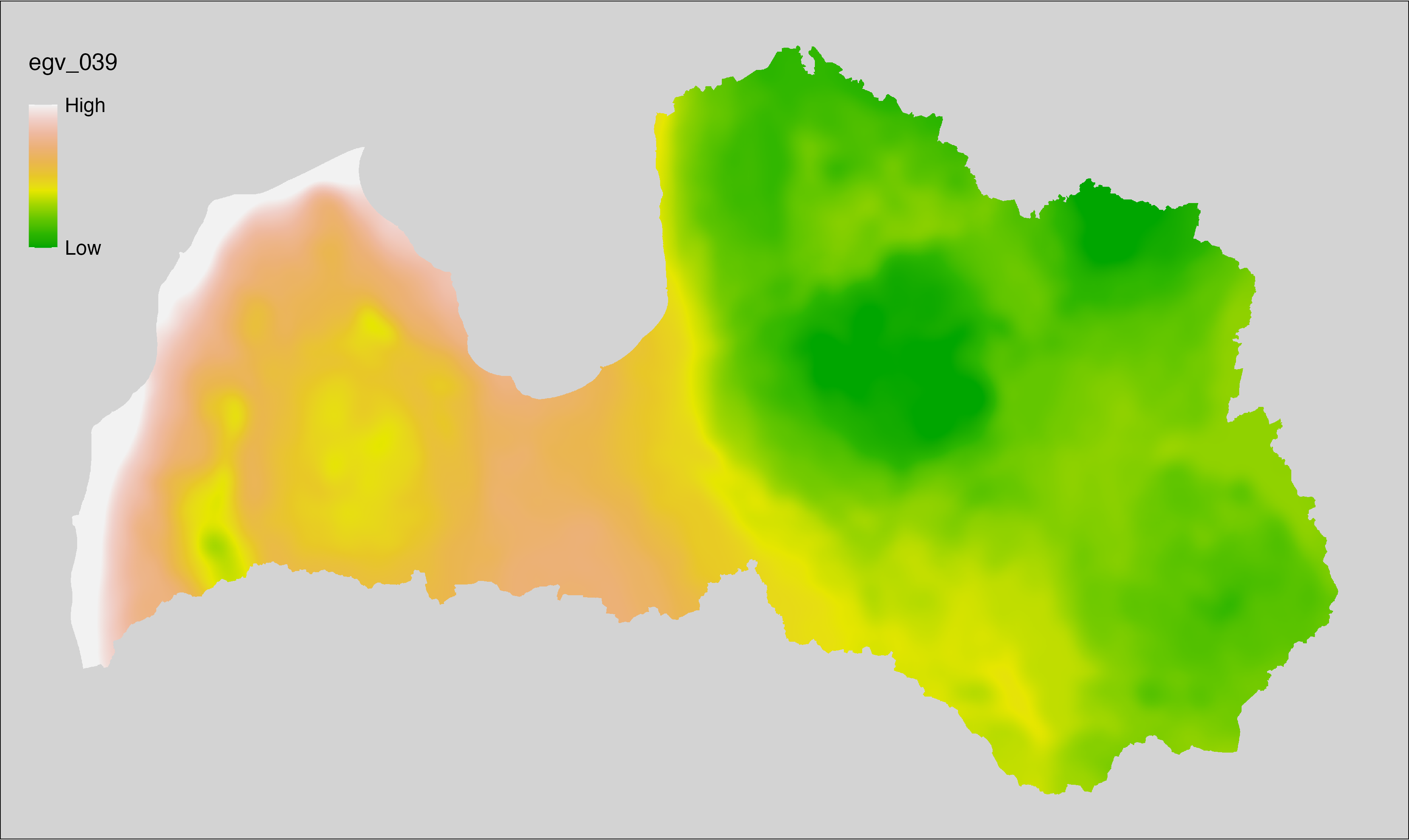
6.40 Climate_CHELSAv2.1-gsp_cell
filename: Climate_CHELSAv2.1-gsp_cell.tif
layername: egv_040
English name: Accumulated precipitation amount (kg m⁻² year⁻¹) on growing season days (TREELIM) (CHELSA v2.1) within the analysis cell (1 ha)
Latvian name: Veģetācijas sezonā (TREELIM) uzkrātais nokrišņu daudzums (kg m⁻² year⁻¹) (CHELSA v2.1) analīzes šūnā (1 ha)
Procedure: Directly follows CHELSA v2.1. EGV is prepared using
the workflow egvtools::downscale2egv() with inverse distance weighted (power =
2) gap filling and soft smoothing (power = 0.5) over 5 km radius around each cell.
Finally, the layer is standardised by subtracting the arithmetic mean and
dividing by the root mean squared error.
Code
# libs ----
if(!require(egvtools)) {remotes::install_github("aavotins/egvtools"); require(egvtools)}
# job ----
localname="Climate_CHELSAv2.1-gsp_cell.tif"
layername="egv_040"
reading="./Geodata/2024/CHELSA/Climate_CHELSAv2.1-gsp_cell.tif"
df <- downscale2egv(
template_path = "./Templates/TemplateRasters/LV100m_10km.tif",
grid_path = "./Templates/TemplateGrids/tikls1km_sauzeme.parquet",
rawfile_path = reading,
out_path = "./RasterGrids_100m/2024/RAW/",
file_name = localname,
layer_name = layername,
fill_gaps = TRUE,
smooth = TRUE,
smooth_radius_km = 5,
plot_result = TRUE)
print(df)
# standardisation ----
if(!require(terra)) {install.packages("terra"); require(terra)}
if(!require(tidyverse)) {install.packages("tidyverse"); require(tidyverse)}
nosaukums="Climate_CHELSAv2.1-gsp_cell.tif"
ielasisanas_cels=paste0("./RasterGrids_100m/2024/RAW/",nosaukums)
saglabasanas_cels=paste0("./RasterGrids_100m/2024/Scaled/",nosaukums)
slanis=rast(ielasisanas_cels)
videjais=global(slanis,fun="mean",na.rm=TRUE)
centrets=slanis-videjais[,1]
standartnovirze=terra::global(centrets,fun="rms",na.rm=TRUE)
merogots=centrets/standartnovirze[,1]
writeRaster(merogots,
filename=saglabasanas_cels,
overwrite=TRUE)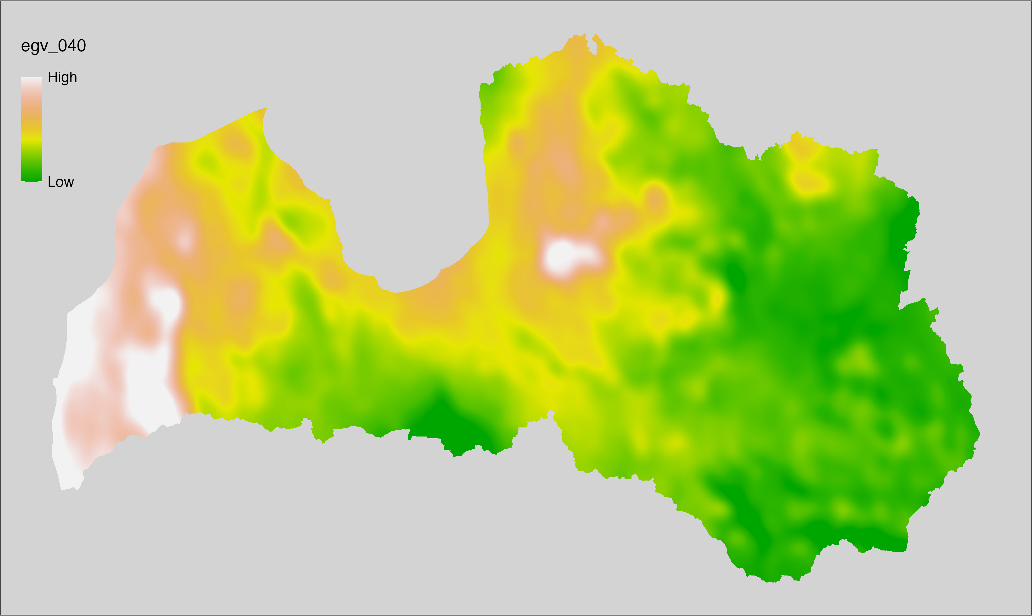
6.41 Climate_CHELSAv2.1-gst_cell
filename: Climate_CHELSAv2.1-gst_cell.tif
layername: egv_041
English name: Mean daily mean air temperature of the growing season (TREELIM) (CHELSA v2.1) within the analysis cell (1 ha)
Latvian name: Vidējā ik dienas vidējā gaisa temperatūra (°C) veģetācijas sezonā (TREELIM) (CHELSA v2.1) analīzes šūnā (1 ha)
Procedure: Directly follows CHELSA v2.1. EGV is prepared using
the workflow egvtools::downscale2egv() with inverse distance weighted (power =
2) gap filling and soft smoothing (power = 0.5) over 5 km radius around each cell.
Finally, the layer is standardised by subtracting the arithmetic mean and
dividing by the root mean squared error.
Code
# libs ----
if(!require(egvtools)) {remotes::install_github("aavotins/egvtools"); require(egvtools)}
# job ----
localname="Climate_CHELSAv2.1-gst_cell.tif"
layername="egv_041"
reading="./Geodata/2024/CHELSA/Climate_CHELSAv2.1-gst_cell.tif"
df <- downscale2egv(
template_path = "./Templates/TemplateRasters/LV100m_10km.tif",
grid_path = "./Templates/TemplateGrids/tikls1km_sauzeme.parquet",
rawfile_path = reading,
out_path = "./RasterGrids_100m/2024/RAW/",
file_name = localname,
layer_name = layername,
fill_gaps = TRUE,
smooth = TRUE,
smooth_radius_km = 5,
plot_result = TRUE)
print(df)
# standardisation ----
if(!require(terra)) {install.packages("terra"); require(terra)}
if(!require(tidyverse)) {install.packages("tidyverse"); require(tidyverse)}
nosaukums="Climate_CHELSAv2.1-gst_cell.tif"
ielasisanas_cels=paste0("./RasterGrids_100m/2024/RAW/",nosaukums)
saglabasanas_cels=paste0("./RasterGrids_100m/2024/Scaled/",nosaukums)
slanis=rast(ielasisanas_cels)
videjais=global(slanis,fun="mean",na.rm=TRUE)
centrets=slanis-videjais[,1]
standartnovirze=terra::global(centrets,fun="rms",na.rm=TRUE)
merogots=centrets/standartnovirze[,1]
writeRaster(merogots,
filename=saglabasanas_cels,
overwrite=TRUE)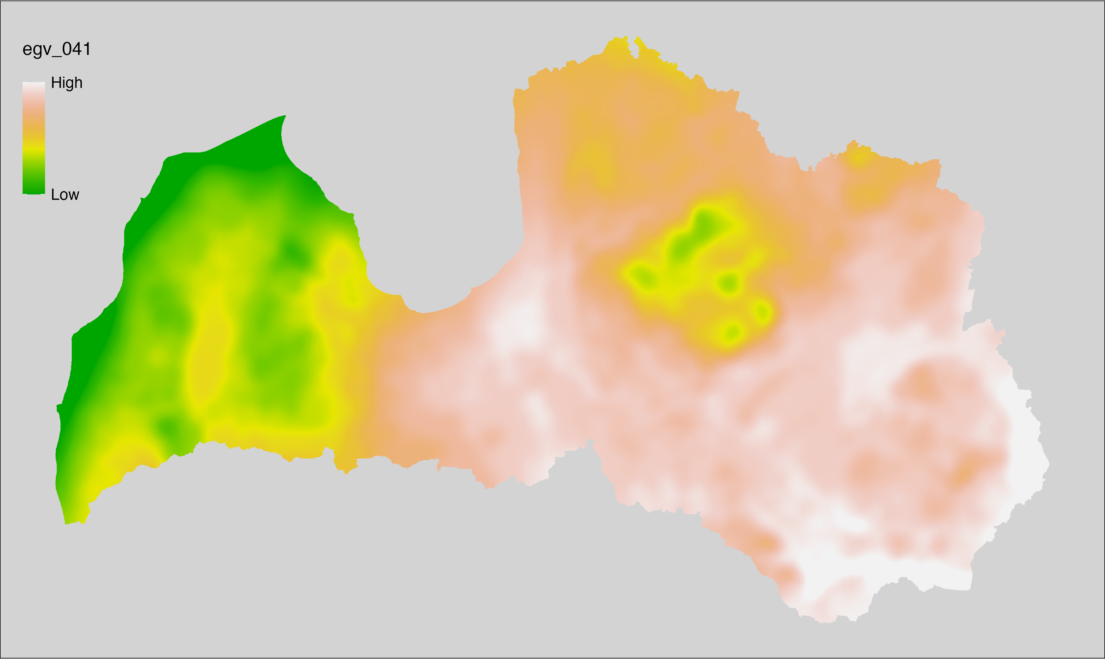
6.42 Climate_CHELSAv2.1-hurs-max_cell
filename: Climate_CHELSAv2.1-hurs-max_cell.tif
layername: egv_042
English name: Mean of monthly maximum near-surface relative humidity (%) (CHELSA v2.1) within the analysis cell (1 ha)
Latvian name: Vidējais ik mēneša maksimālais piezemes slāņa gaisa mitrums (%) (CHELSA v2.1) analīzes šūnā (1 ha)
Procedure: Directly follows CHELSA v2.1. EGV is prepared using
the workflow egvtools::downscale2egv() with inverse distance weighted (power =
2) gap filling and soft smoothing (power = 0.5) over 5 km radius around each cell.
Finally, the layer is standardised by subtracting the arithmetic mean and
dividing by the root mean squared error.
Code
# libs ----
if(!require(egvtools)) {remotes::install_github("aavotins/egvtools"); require(egvtools)}
# job ----
localname="Climate_CHELSAv2.1-hurs-max_cell.tif"
layername="egv_042"
reading="./Geodata/2024/CHELSA/Climate_CHELSAv2.1-hurs-max_cell.tif"
df <- downscale2egv(
template_path = "./Templates/TemplateRasters/LV100m_10km.tif",
grid_path = "./Templates/TemplateGrids/tikls1km_sauzeme.parquet",
rawfile_path = reading,
out_path = "./RasterGrids_100m/2024/RAW/",
file_name = localname,
layer_name = layername,
fill_gaps = TRUE,
smooth = TRUE,
smooth_radius_km = 5,
plot_result = TRUE)
print(df)
# standardisation ----
if(!require(terra)) {install.packages("terra"); require(terra)}
if(!require(tidyverse)) {install.packages("tidyverse"); require(tidyverse)}
nosaukums="Climate_CHELSAv2.1-hurs-max_cell.tif"
ielasisanas_cels=paste0("./RasterGrids_100m/2024/RAW/",nosaukums)
saglabasanas_cels=paste0("./RasterGrids_100m/2024/Scaled/",nosaukums)
slanis=rast(ielasisanas_cels)
videjais=global(slanis,fun="mean",na.rm=TRUE)
centrets=slanis-videjais[,1]
standartnovirze=terra::global(centrets,fun="rms",na.rm=TRUE)
merogots=centrets/standartnovirze[,1]
writeRaster(merogots,
filename=saglabasanas_cels,
overwrite=TRUE)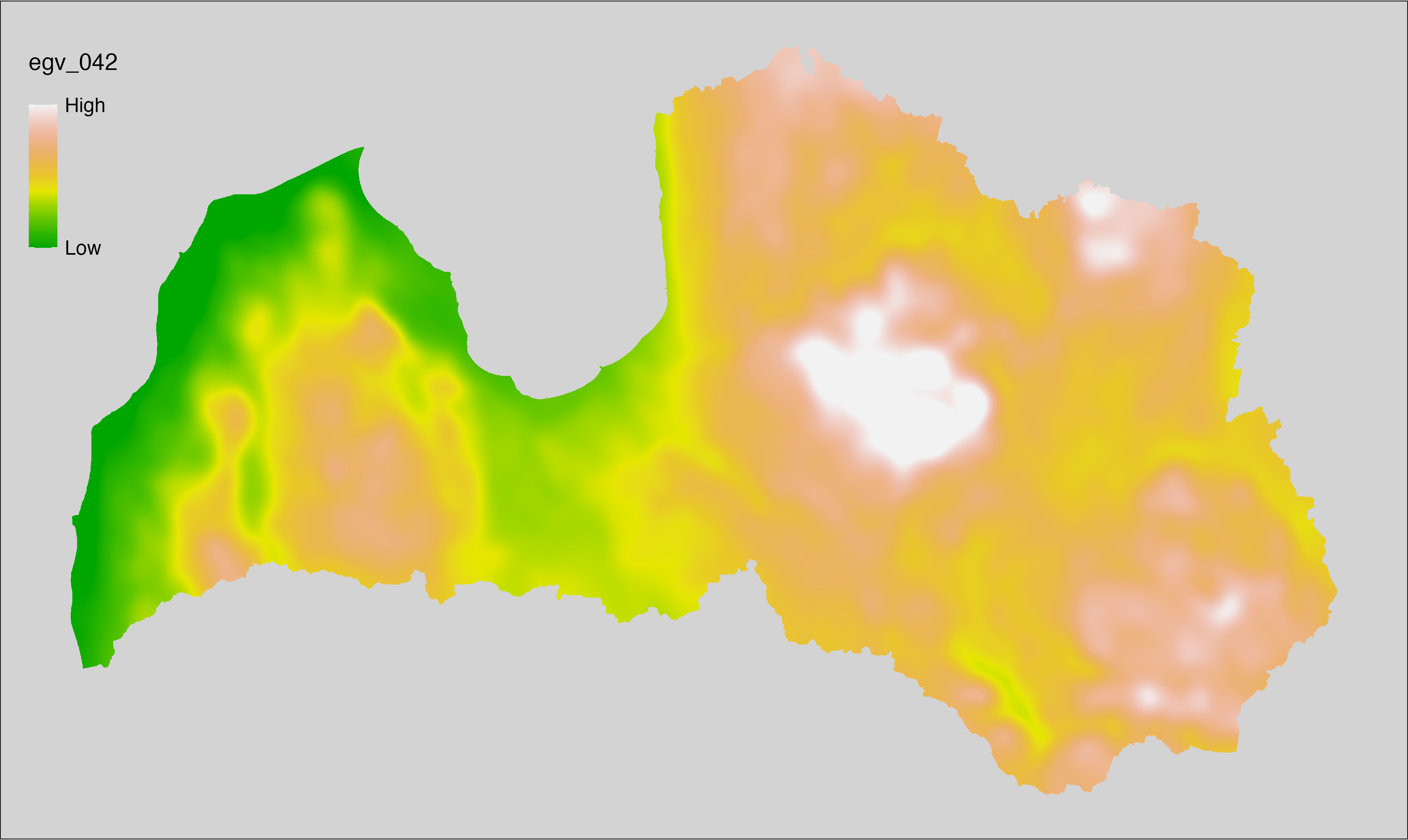
6.43 Climate_CHELSAv2.1-hurs-mean_cell
filename: Climate_CHELSAv2.1-hurs-mean_cell.tif
layername: egv_043
English name: Mean of monthly mean near-surface relative humidity (%) (CHELSA v2.1) within the analysis cell (1 ha)
Latvian name: Vidējais ik mēneša vidējais piezemes slāņa gaisa mitrums (%) (CHELSA v2.1) analīzes šūnā (1 ha)
Procedure: Directly follows CHELSA v2.1. EGV is prepared using
the workflow egvtools::downscale2egv() with inverse distance weighted (power =
2) gap filling and soft smoothing (power = 0.5) over 5 km radius around each cell.
Finally, the layer is standardised by subtracting the arithmetic mean and
dividing by the root mean squared error.
Code
# libs ----
if(!require(egvtools)) {remotes::install_github("aavotins/egvtools"); require(egvtools)}
# job ----
localname="Climate_CHELSAv2.1-hurs-mean_cell.tif"
layername="egv_043"
reading="./Geodata/2024/CHELSA/Climate_CHELSAv2.1-hurs-mean_cell.tif"
df <- downscale2egv(
template_path = "./Templates/TemplateRasters/LV100m_10km.tif",
grid_path = "./Templates/TemplateGrids/tikls1km_sauzeme.parquet",
rawfile_path = reading,
out_path = "./RasterGrids_100m/2024/RAW/",
file_name = localname,
layer_name = layername,
fill_gaps = TRUE,
smooth = TRUE,
smooth_radius_km = 5,
plot_result = TRUE)
print(df)
# standardisation ----
if(!require(terra)) {install.packages("terra"); require(terra)}
if(!require(tidyverse)) {install.packages("tidyverse"); require(tidyverse)}
nosaukums="Climate_CHELSAv2.1-hurs-mean_cell.tif"
ielasisanas_cels=paste0("./RasterGrids_100m/2024/RAW/",nosaukums)
saglabasanas_cels=paste0("./RasterGrids_100m/2024/Scaled/",nosaukums)
slanis=rast(ielasisanas_cels)
videjais=global(slanis,fun="mean",na.rm=TRUE)
centrets=slanis-videjais[,1]
standartnovirze=terra::global(centrets,fun="rms",na.rm=TRUE)
merogots=centrets/standartnovirze[,1]
writeRaster(merogots,
filename=saglabasanas_cels,
overwrite=TRUE)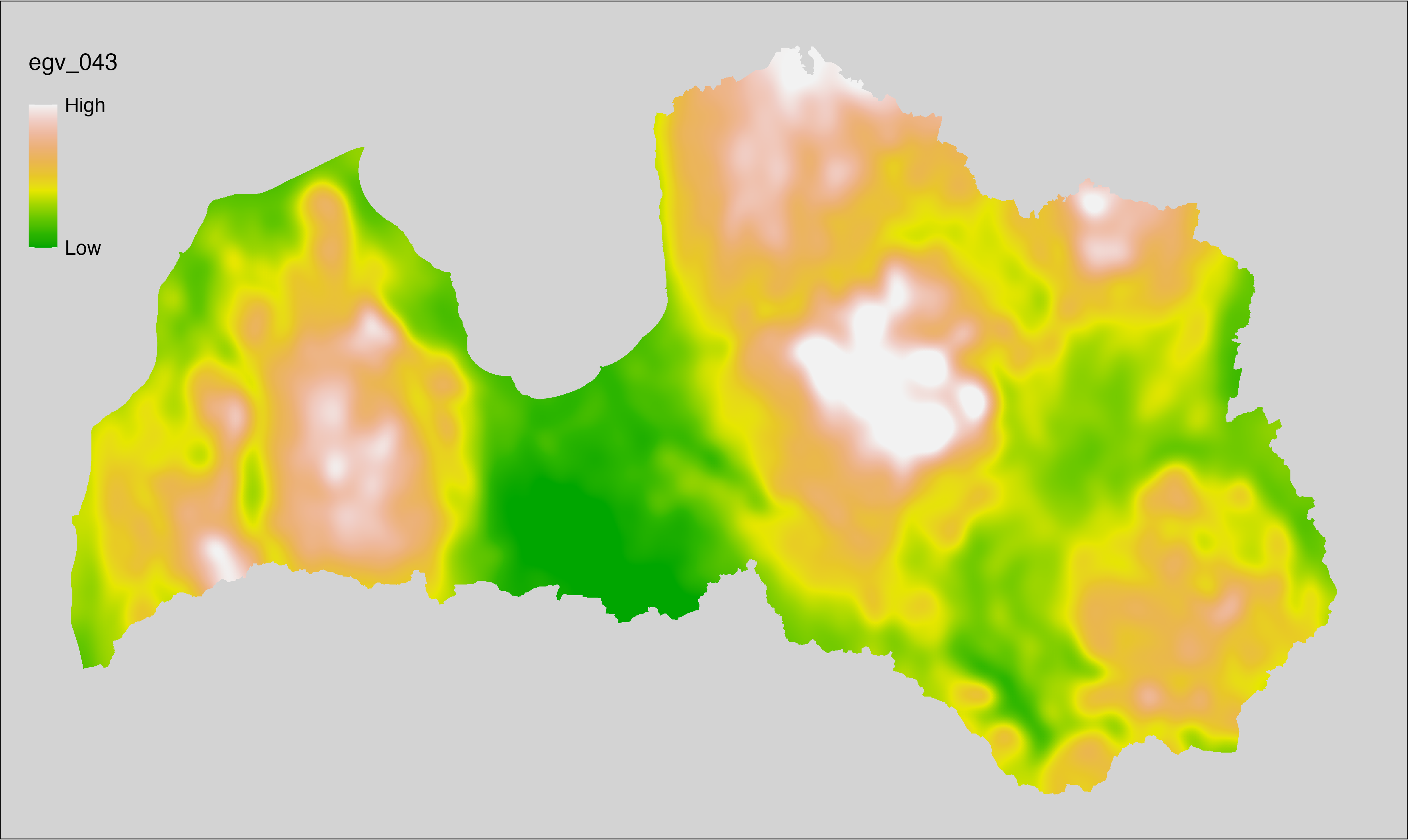
6.44 Climate_CHELSAv2.1-hurs-min_cell
filename: Climate_CHELSAv2.1-hurs-min_cell.tif
layername: egv_044
English name: Mean of monthly minimum near-surface relative humidity (%) (CHELSA v2.1) within the analysis cell (1 ha)
Latvian name: Vidējais ik mēneša minimālais gaisa mitrums (%) (CHELSA v2.1) analīzes šūnā (1 ha)
Procedure: Directly follows CHELSA v2.1. EGV is prepared using
the workflow egvtools::downscale2egv() with inverse distance weighted (power =
2) gap filling and soft smoothing (power = 0.5) over 5 km radius around each cell.
Finally, the layer is standardised by subtracting the arithmetic mean and
dividing by the root mean squared error.
Code
# libs ----
if(!require(egvtools)) {remotes::install_github("aavotins/egvtools"); require(egvtools)}
# job ----
localname="Climate_CHELSAv2.1-hurs-min_cell.tif"
layername="egv_044"
reading="./Geodata/2024/CHELSA/Climate_CHELSAv2.1-hurs-min_cell.tif"
df <- downscale2egv(
template_path = "./Templates/TemplateRasters/LV100m_10km.tif",
grid_path = "./Templates/TemplateGrids/tikls1km_sauzeme.parquet",
rawfile_path = reading,
out_path = "./RasterGrids_100m/2024/RAW/",
file_name = localname,
layer_name = layername,
fill_gaps = TRUE,
smooth = TRUE,
smooth_radius_km = 5,
plot_result = TRUE)
print(df)
# standardisation ----
if(!require(terra)) {install.packages("terra"); require(terra)}
if(!require(tidyverse)) {install.packages("tidyverse"); require(tidyverse)}
nosaukums="Climate_CHELSAv2.1-hurs-min_cell.tif"
ielasisanas_cels=paste0("./RasterGrids_100m/2024/RAW/",nosaukums)
saglabasanas_cels=paste0("./RasterGrids_100m/2024/Scaled/",nosaukums)
slanis=rast(ielasisanas_cels)
videjais=global(slanis,fun="mean",na.rm=TRUE)
centrets=slanis-videjais[,1]
standartnovirze=terra::global(centrets,fun="rms",na.rm=TRUE)
merogots=centrets/standartnovirze[,1]
writeRaster(merogots,
filename=saglabasanas_cels,
overwrite=TRUE)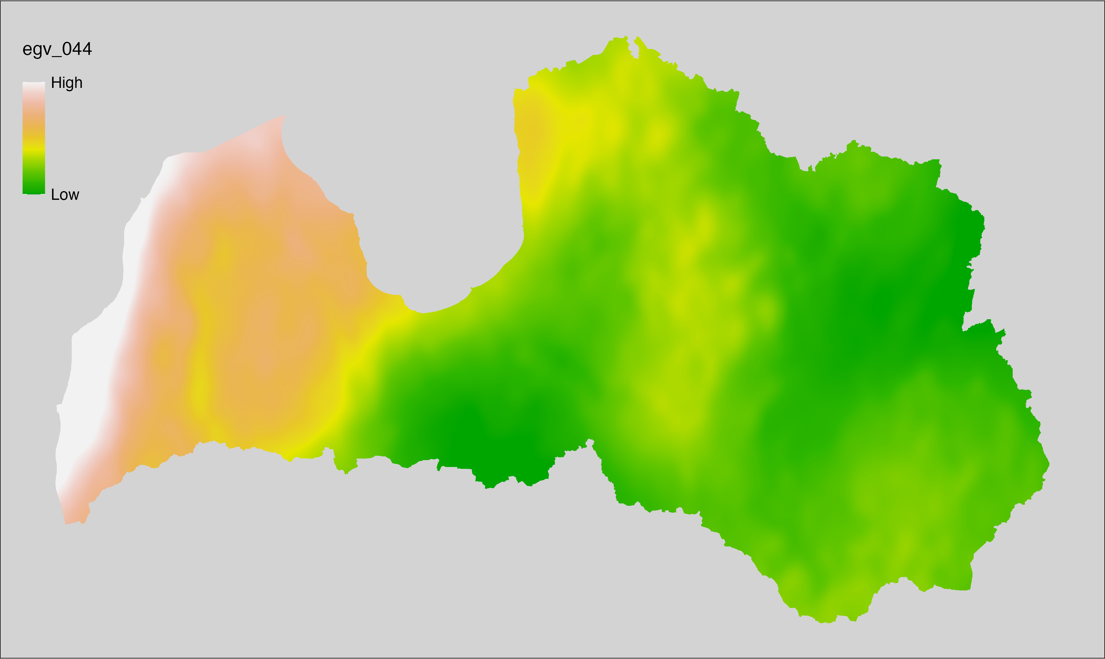
6.45 Climate_CHELSAv2.1-hurs-range_cell
filename: Climate_CHELSAv2.1-hurs-range_cell.tif
layername: egv_045
English name: Annual range of monthly near-surface relative humidity (%) (CHELSA v2.1) within the analysis cell (1 ha)
Latvian name: Gada gaisa mitruma piezemes slānī amplitūda (%) (CHELSA v2.1) analīzes šūnā (1 ha)
Procedure: Directly follows CHELSA v2.1. EGV is prepared using
the workflow egvtools::downscale2egv() with inverse distance weighted (power =
2) gap filling and soft smoothing (power = 0.5) over 5 km radius around each cell.
Finally, the layer is standardised by subtracting the arithmetic mean and
dividing by the root mean squared error.
Code
# libs ----
if(!require(egvtools)) {remotes::install_github("aavotins/egvtools"); require(egvtools)}
# job ----
localname="Climate_CHELSAv2.1-hurs-range_cell.tif"
layername="egv_045"
reading="./Geodata/2024/CHELSA/Climate_CHELSAv2.1-hurs-range_cell.tif"
df <- downscale2egv(
template_path = "./Templates/TemplateRasters/LV100m_10km.tif",
grid_path = "./Templates/TemplateGrids/tikls1km_sauzeme.parquet",
rawfile_path = reading,
out_path = "./RasterGrids_100m/2024/RAW/",
file_name = localname,
layer_name = layername,
fill_gaps = TRUE,
smooth = TRUE,
smooth_radius_km = 5,
plot_result = TRUE)
print(df)
# standardisation ----
if(!require(terra)) {install.packages("terra"); require(terra)}
if(!require(tidyverse)) {install.packages("tidyverse"); require(tidyverse)}
nosaukums="Climate_CHELSAv2.1-hurs-range_cell.tif"
ielasisanas_cels=paste0("./RasterGrids_100m/2024/RAW/",nosaukums)
saglabasanas_cels=paste0("./RasterGrids_100m/2024/Scaled/",nosaukums)
slanis=rast(ielasisanas_cels)
videjais=global(slanis,fun="mean",na.rm=TRUE)
centrets=slanis-videjais[,1]
standartnovirze=terra::global(centrets,fun="rms",na.rm=TRUE)
merogots=centrets/standartnovirze[,1]
writeRaster(merogots,
filename=saglabasanas_cels,
overwrite=TRUE)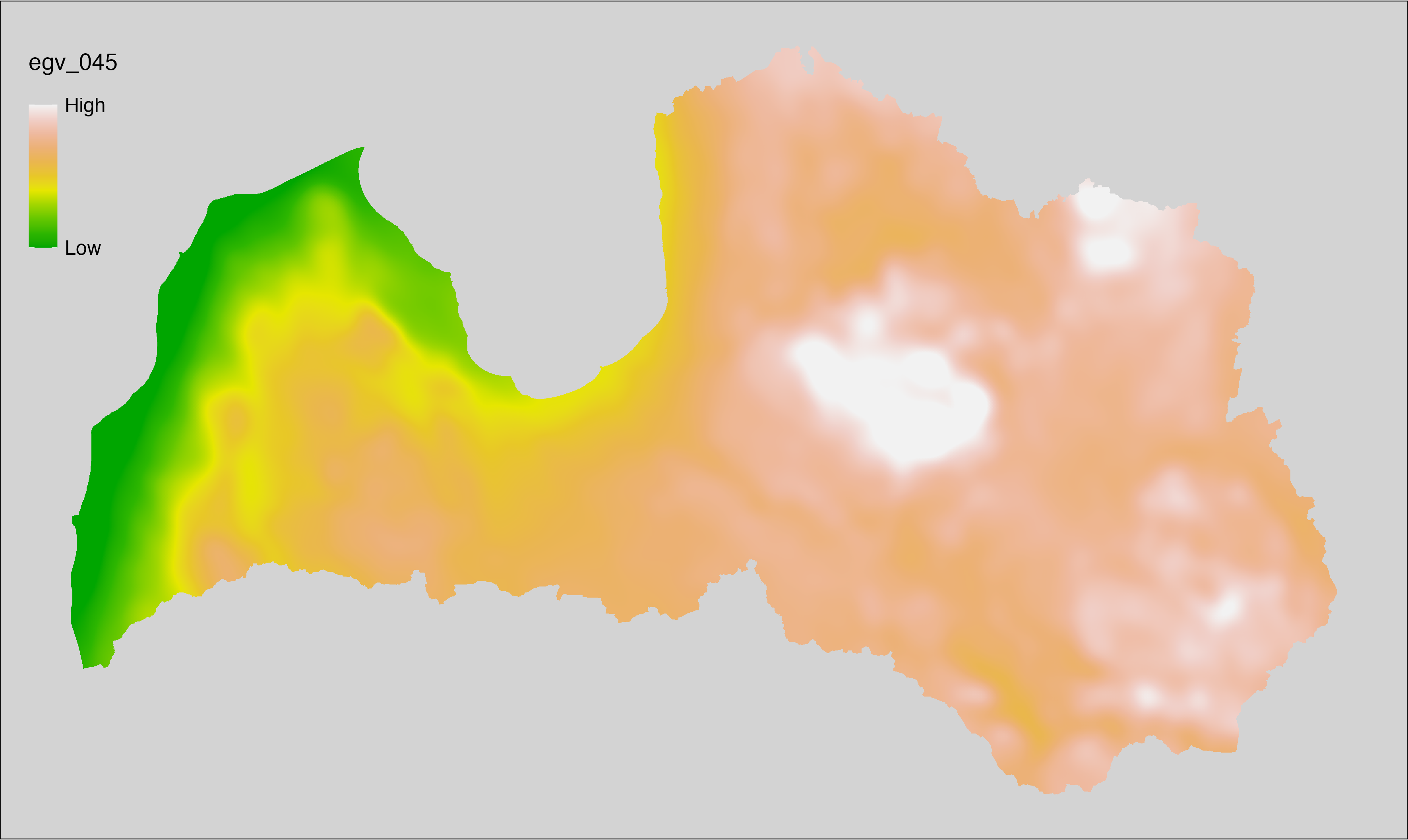
6.46 Climate_CHELSAv2.1-lgd_cell
filename: Climate_CHELSAv2.1-lgd_cell.tif
layername: egv_046
English name: Last day of the growing season (TREELIM) (CHELSA v2.1) within the analysis cell (1 ha)
Latvian name: Pēdējā veģetācijas sezonas diena (TREELIM) (CHELSA v2.1) analīzes šūnā (1 ha)
Procedure: Directly follows CHELSA v2.1. EGV is prepared using
the workflow egvtools::downscale2egv() with inverse distance weighted (power =
2) gap filling and soft smoothing (power = 0.5) over 5 km radius around each cell.
Finally, the layer is standardised by subtracting the arithmetic mean and
dividing by the root mean squared error.
Code
# libs ----
if(!require(egvtools)) {remotes::install_github("aavotins/egvtools"); require(egvtools)}
# job ----
localname="Climate_CHELSAv2.1-lgd_cell.tif"
layername="egv_046"
reading="./Geodata/2024/CHELSA/Climate_CHELSAv2.1-lgd_cell.tif"
df <- downscale2egv(
template_path = "./Templates/TemplateRasters/LV100m_10km.tif",
grid_path = "./Templates/TemplateGrids/tikls1km_sauzeme.parquet",
rawfile_path = reading,
out_path = "./RasterGrids_100m/2024/RAW/",
file_name = localname,
layer_name = layername,
fill_gaps = TRUE,
smooth = TRUE,
smooth_radius_km = 5,
plot_result = TRUE)
print(df)
# standardisation ----
if(!require(terra)) {install.packages("terra"); require(terra)}
if(!require(tidyverse)) {install.packages("tidyverse"); require(tidyverse)}
nosaukums="Climate_CHELSAv2.1-lgd_cell.tif"
ielasisanas_cels=paste0("./RasterGrids_100m/2024/RAW/",nosaukums)
saglabasanas_cels=paste0("./RasterGrids_100m/2024/Scaled/",nosaukums)
slanis=rast(ielasisanas_cels)
videjais=global(slanis,fun="mean",na.rm=TRUE)
centrets=slanis-videjais[,1]
standartnovirze=terra::global(centrets,fun="rms",na.rm=TRUE)
merogots=centrets/standartnovirze[,1]
writeRaster(merogots,
filename=saglabasanas_cels,
overwrite=TRUE)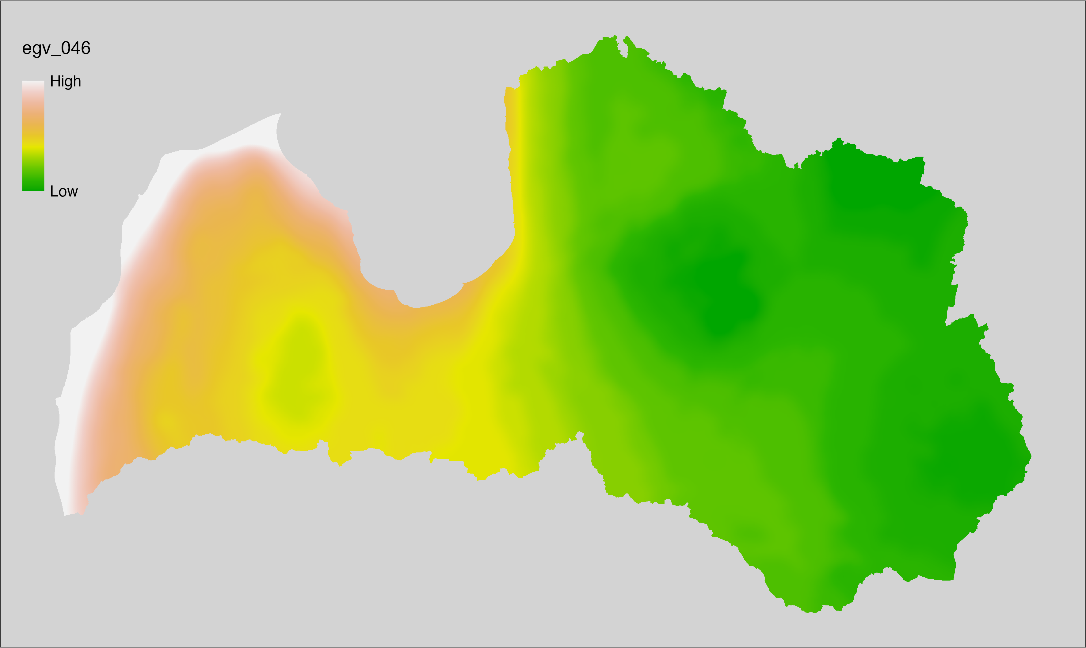
6.47 Climate_CHELSAv2.1-ngd0_cell
filename: Climate_CHELSAv2.1-ngd0_cell.tif
layername: egv_047
English name: Number of days in which air temperature at 2 m is > 0°C (CHELSA v2.1) within the analysis cell (1 ha)
Latvian name: Dienu skaits, kurā gaisa temperatūra 2 m augstumā pārsniedz 0°C (CHELSA v2.1) analīzes šūnā (1 ha)
Procedure: Directly follows CHELSA v2.1. EGV is prepared using
the workflow egvtools::downscale2egv() with inverse distance weighted (power =
2) gap filling and soft smoothing (power = 0.5) over 5 km radius around each cell.
Finally, the layer is standardised by subtracting the arithmetic mean and
dividing by the root mean squared error.
Code
# libs ----
if(!require(egvtools)) {remotes::install_github("aavotins/egvtools"); require(egvtools)}
# job ----
localname="Climate_CHELSAv2.1-ngd0_cell.tif"
layername="egv_047"
reading="./Geodata/2024/CHELSA/Climate_CHELSAv2.1-ngd0_cell.tif"
df <- downscale2egv(
template_path = "./Templates/TemplateRasters/LV100m_10km.tif",
grid_path = "./Templates/TemplateGrids/tikls1km_sauzeme.parquet",
rawfile_path = reading,
out_path = "./RasterGrids_100m/2024/RAW/",
file_name = localname,
layer_name = layername,
fill_gaps = TRUE,
smooth = TRUE,
smooth_radius_km = 5,
plot_result = TRUE)
print(df)
# standardisation ----
if(!require(terra)) {install.packages("terra"); require(terra)}
if(!require(tidyverse)) {install.packages("tidyverse"); require(tidyverse)}
nosaukums="Climate_CHELSAv2.1-ngd0_cell.tif"
ielasisanas_cels=paste0("./RasterGrids_100m/2024/RAW/",nosaukums)
saglabasanas_cels=paste0("./RasterGrids_100m/2024/Scaled/",nosaukums)
slanis=rast(ielasisanas_cels)
videjais=global(slanis,fun="mean",na.rm=TRUE)
centrets=slanis-videjais[,1]
standartnovirze=terra::global(centrets,fun="rms",na.rm=TRUE)
merogots=centrets/standartnovirze[,1]
writeRaster(merogots,
filename=saglabasanas_cels,
overwrite=TRUE)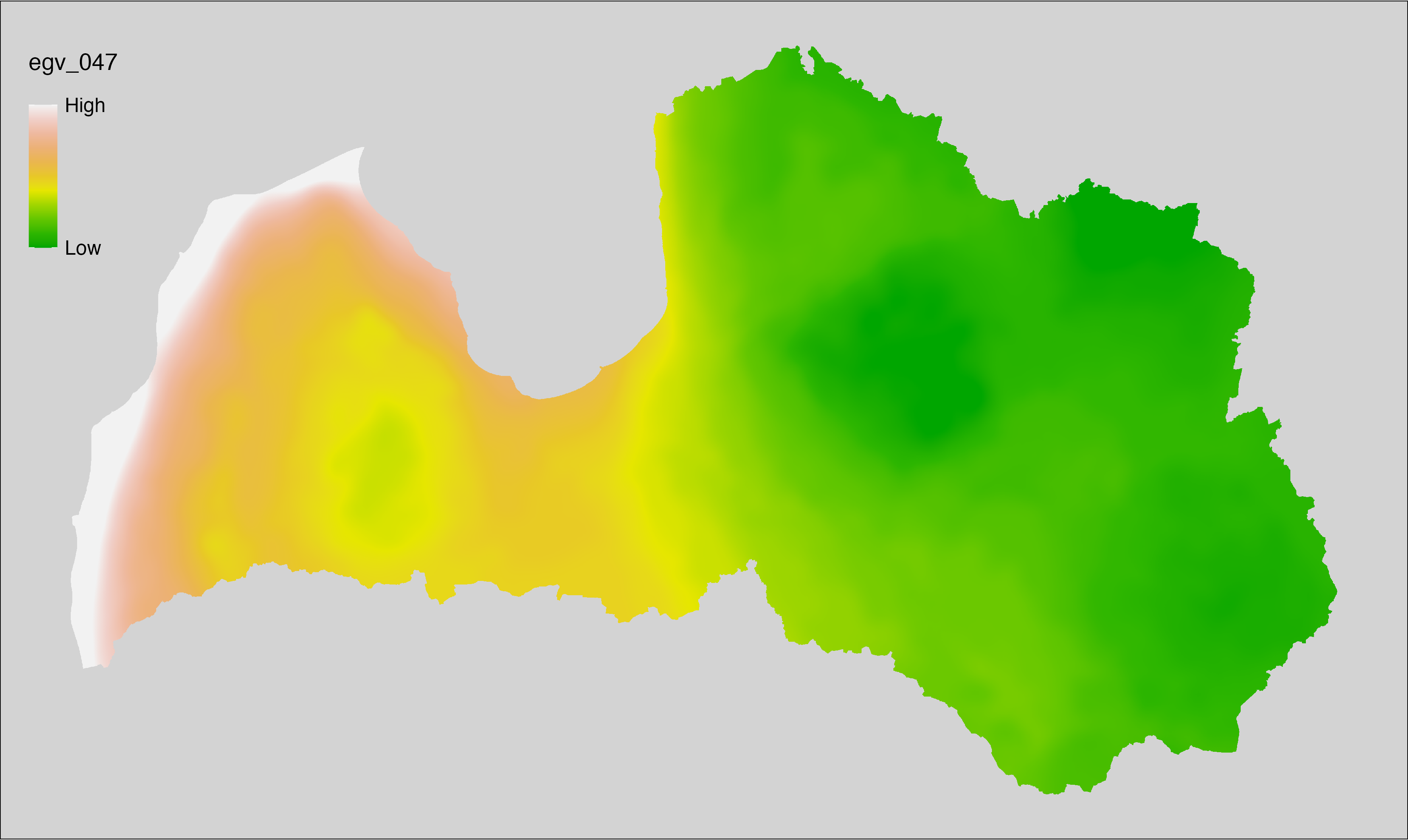
6.48 Climate_CHELSAv2.1-ngd10_cell
filename: Climate_CHELSAv2.1-ngd10_cell.tif
layername: egv_048
English name: Number of days in which air temperature at 2 m is > 10°C (CHELSA v2.1) within the analysis cell (1 ha)
Latvian name: Dienu skaits, kurā gaisa temperatūra 2 m augstumā pārsniedz 10°C (CHELSA v2.1) analīzes šūnā (1 ha)
Procedure: Directly follows CHELSA v2.1. EGV is prepared using
the workflow egvtools::downscale2egv() with inverse distance weighted (power =
2) gap filling and soft smoothing (power = 0.5) over 5 km radius around each cell.
Finally, the layer is standardised by subtracting the arithmetic mean and
dividing by the root mean squared error.
Code
# libs ----
if(!require(egvtools)) {remotes::install_github("aavotins/egvtools"); require(egvtools)}
# job ----
localname="Climate_CHELSAv2.1-ngd10_cell.tif"
layername="egv_048"
reading="./Geodata/2024/CHELSA/Climate_CHELSAv2.1-ngd10_cell.tif"
df <- downscale2egv(
template_path = "./Templates/TemplateRasters/LV100m_10km.tif",
grid_path = "./Templates/TemplateGrids/tikls1km_sauzeme.parquet",
rawfile_path = reading,
out_path = "./RasterGrids_100m/2024/RAW/",
file_name = localname,
layer_name = layername,
fill_gaps = TRUE,
smooth = TRUE,
smooth_radius_km = 5,
plot_result = TRUE)
print(df)
# standardisation ----
if(!require(terra)) {install.packages("terra"); require(terra)}
if(!require(tidyverse)) {install.packages("tidyverse"); require(tidyverse)}
nosaukums="Climate_CHELSAv2.1-ngd10_cell.tif"
ielasisanas_cels=paste0("./RasterGrids_100m/2024/RAW/",nosaukums)
saglabasanas_cels=paste0("./RasterGrids_100m/2024/Scaled/",nosaukums)
slanis=rast(ielasisanas_cels)
videjais=global(slanis,fun="mean",na.rm=TRUE)
centrets=slanis-videjais[,1]
standartnovirze=terra::global(centrets,fun="rms",na.rm=TRUE)
merogots=centrets/standartnovirze[,1]
writeRaster(merogots,
filename=saglabasanas_cels,
overwrite=TRUE)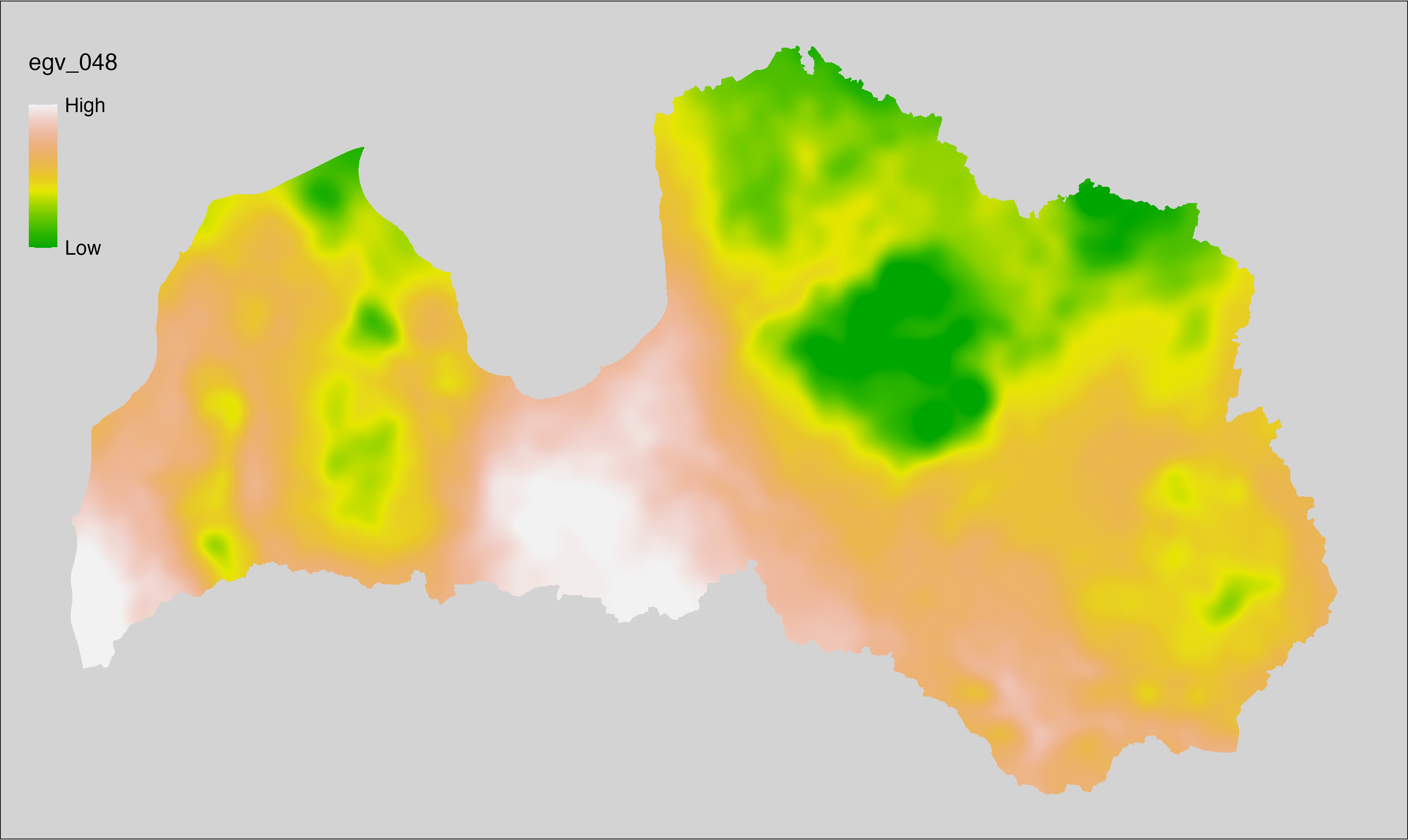
6.49 Climate_CHELSAv2.1-ngd5_cell
filename: Climate_CHELSAv2.1-ngd5_cell.tif
layername: egv_049
English name: Number of days in which air temperature at 2 m is > 5°C (CHELSA v2.1) within the analysis cell (1 ha)
Latvian name: Dienu skaits, kurā gaisa temperatūra 2 m augstumā pārsniedz 5°C (CHELSA v2.1) analīzes šūnā (1 ha)
Procedure: Directly follows CHELSA v2.1. EGV is prepared using
the workflow egvtools::downscale2egv() with inverse distance weighted (power =
2) gap filling and soft smoothing (power = 0.5) over 5 km radius around each cell.
Finally, the layer is standardised by subtracting the arithmetic mean and
dividing by the root mean squared error.
Code
# libs ----
if(!require(egvtools)) {remotes::install_github("aavotins/egvtools"); require(egvtools)}
# job ----
localname="Climate_CHELSAv2.1-ngd5_cell.tif"
layername="egv_049"
reading="./Geodata/2024/CHELSA/Climate_CHELSAv2.1-ngd5_cell.tif"
df <- downscale2egv(
template_path = "./Templates/TemplateRasters/LV100m_10km.tif",
grid_path = "./Templates/TemplateGrids/tikls1km_sauzeme.parquet",
rawfile_path = reading,
out_path = "./RasterGrids_100m/2024/RAW/",
file_name = localname,
layer_name = layername,
fill_gaps = TRUE,
smooth = TRUE,
smooth_radius_km = 5,
plot_result = TRUE)
print(df)
# standardisation ----
if(!require(terra)) {install.packages("terra"); require(terra)}
if(!require(tidyverse)) {install.packages("tidyverse"); require(tidyverse)}
nosaukums="Climate_CHELSAv2.1-ngd5_cell.tif"
ielasisanas_cels=paste0("./RasterGrids_100m/2024/RAW/",nosaukums)
saglabasanas_cels=paste0("./RasterGrids_100m/2024/Scaled/",nosaukums)
slanis=rast(ielasisanas_cels)
videjais=global(slanis,fun="mean",na.rm=TRUE)
centrets=slanis-videjais[,1]
standartnovirze=terra::global(centrets,fun="rms",na.rm=TRUE)
merogots=centrets/standartnovirze[,1]
writeRaster(merogots,
filename=saglabasanas_cels,
overwrite=TRUE)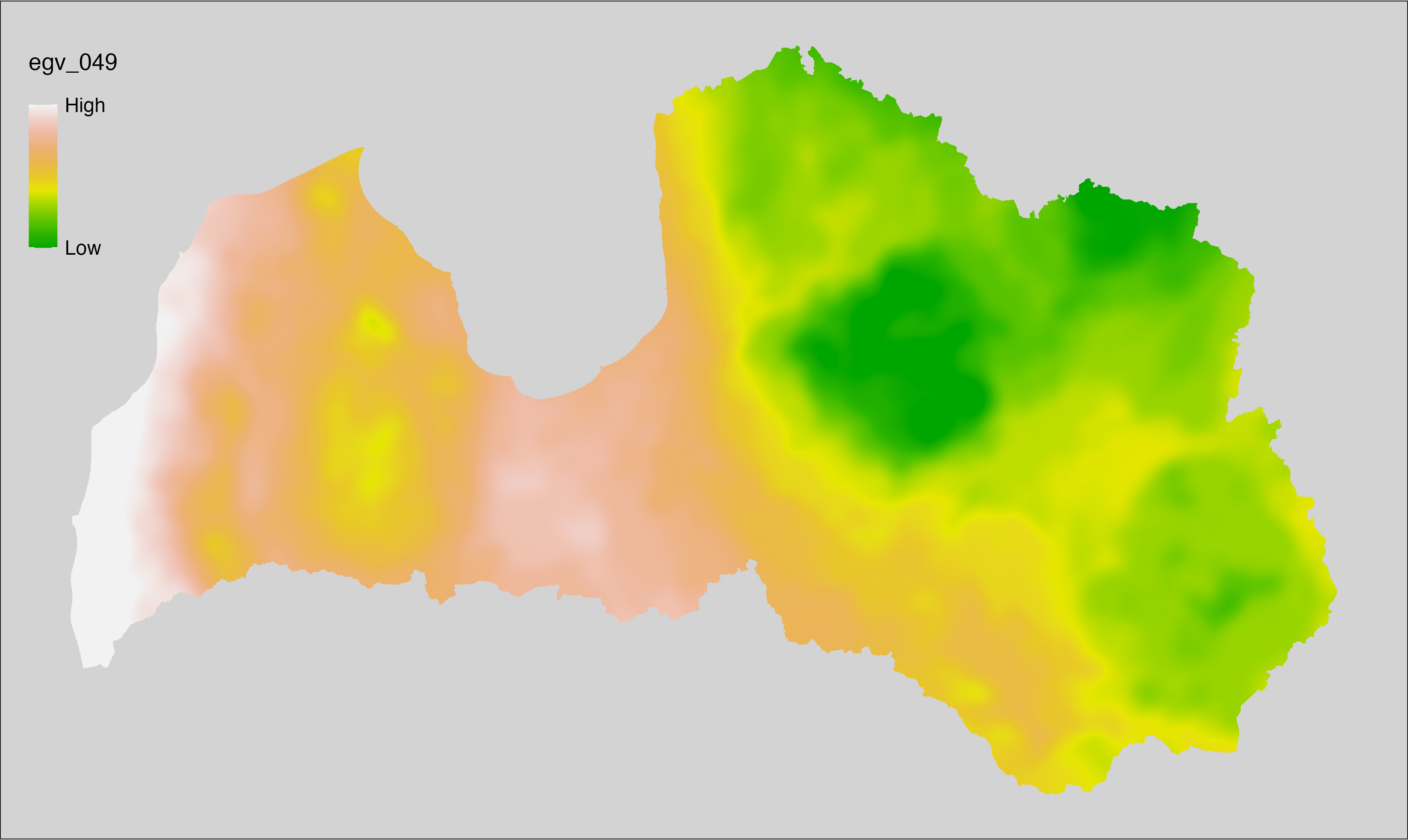
6.50 Climate_CHELSAv2.1-npp_cell
filename: Climate_CHELSAv2.1-npp_cell.tif
layername: egv_050
English name: Net primary productivity (g C m⁻² year⁻¹) (CHELSA v2.1) within the analysis cell (1 ha)
Latvian name: Neto primārā produkcija (g C m⁻² year⁻¹) (CHELSA v2.1) analīzes šūnā (1 ha)
Procedure: Directly follows CHELSA v2.1. EGV is prepared using
the workflow egvtools::downscale2egv() with inverse distance weighted (power =
2) gap filling and soft smoothing (power = 0.5) over 5 km radius around each cell.
Finally, the layer is standardised by subtracting the arithmetic mean and
dividing by the root mean squared error.
Code
# libs ----
if(!require(egvtools)) {remotes::install_github("aavotins/egvtools"); require(egvtools)}
# job ----
localname="Climate_CHELSAv2.1-npp_cell.tif"
layername="egv_050"
reading="./Geodata/2024/CHELSA/Climate_CHELSAv2.1-npp_cell.tif"
df <- downscale2egv(
template_path = "./Templates/TemplateRasters/LV100m_10km.tif",
grid_path = "./Templates/TemplateGrids/tikls1km_sauzeme.parquet",
rawfile_path = reading,
out_path = "./RasterGrids_100m/2024/RAW/",
file_name = localname,
layer_name = layername,
fill_gaps = TRUE,
smooth = TRUE,
smooth_radius_km = 5,
plot_result = TRUE)
print(df)
# standardisation ----
if(!require(terra)) {install.packages("terra"); require(terra)}
if(!require(tidyverse)) {install.packages("tidyverse"); require(tidyverse)}
nosaukums="Climate_CHELSAv2.1-npp_cell.tif"
ielasisanas_cels=paste0("./RasterGrids_100m/2024/RAW/",nosaukums)
saglabasanas_cels=paste0("./RasterGrids_100m/2024/Scaled/",nosaukums)
slanis=rast(ielasisanas_cels)
videjais=global(slanis,fun="mean",na.rm=TRUE)
centrets=slanis-videjais[,1]
standartnovirze=terra::global(centrets,fun="rms",na.rm=TRUE)
merogots=centrets/standartnovirze[,1]
writeRaster(merogots,
filename=saglabasanas_cels,
overwrite=TRUE)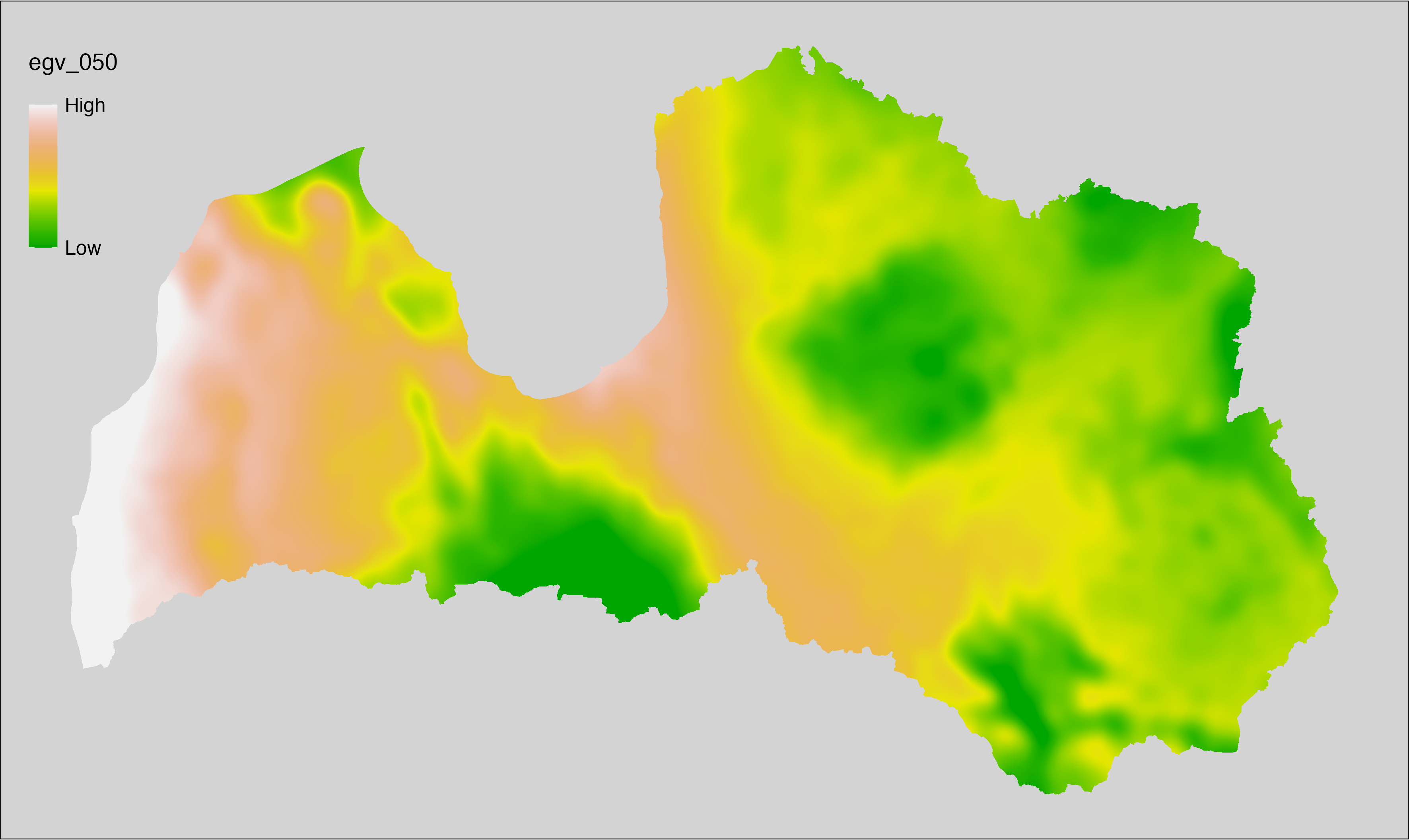
6.51 Climate_CHELSAv2.1-pet-penman-max_cell
filename: Climate_CHELSAv2.1-pet-penman-max_cell.tif
layername: egv_051
English name: Mean of monthly maximum potential evapotranspiration (kg m⁻² month⁻¹) (CHELSA v2.1) within the analysis cell (1 ha)
Latvian name: Vidējā ik mēneša maksimālā potenciālā evapotranspirācija (kg m⁻² month⁻¹) (CHELSA v2.1) analīzes šūnā (1 ha)
Procedure: Directly follows CHELSA v2.1. EGV is prepared using
the workflow egvtools::downscale2egv() with inverse distance weighted (power =
2) gap filling and soft smoothing (power = 0.5) over 5 km radius around each cell.
Finally, the layer is standardised by subtracting the arithmetic mean and
dividing by the root mean squared error.
Code
# libs ----
if(!require(egvtools)) {remotes::install_github("aavotins/egvtools"); require(egvtools)}
# job ----
localname="Climate_CHELSAv2.1-pet-penman-max_cell.tif"
layername="egv_051"
reading="./Geodata/2024/CHELSA/Climate_CHELSAv2.1-pet-penman-max_cell.tif"
df <- downscale2egv(
template_path = "./Templates/TemplateRasters/LV100m_10km.tif",
grid_path = "./Templates/TemplateGrids/tikls1km_sauzeme.parquet",
rawfile_path = reading,
out_path = "./RasterGrids_100m/2024/RAW/",
file_name = localname,
layer_name = layername,
fill_gaps = TRUE,
smooth = TRUE,
smooth_radius_km = 5,
plot_result = TRUE)
print(df)
# standardisation ----
if(!require(terra)) {install.packages("terra"); require(terra)}
if(!require(tidyverse)) {install.packages("tidyverse"); require(tidyverse)}
nosaukums="Climate_CHELSAv2.1-pet-penman-max_cell.tif"
ielasisanas_cels=paste0("./RasterGrids_100m/2024/RAW/",nosaukums)
saglabasanas_cels=paste0("./RasterGrids_100m/2024/Scaled/",nosaukums)
slanis=rast(ielasisanas_cels)
videjais=global(slanis,fun="mean",na.rm=TRUE)
centrets=slanis-videjais[,1]
standartnovirze=terra::global(centrets,fun="rms",na.rm=TRUE)
merogots=centrets/standartnovirze[,1]
writeRaster(merogots,
filename=saglabasanas_cels,
overwrite=TRUE)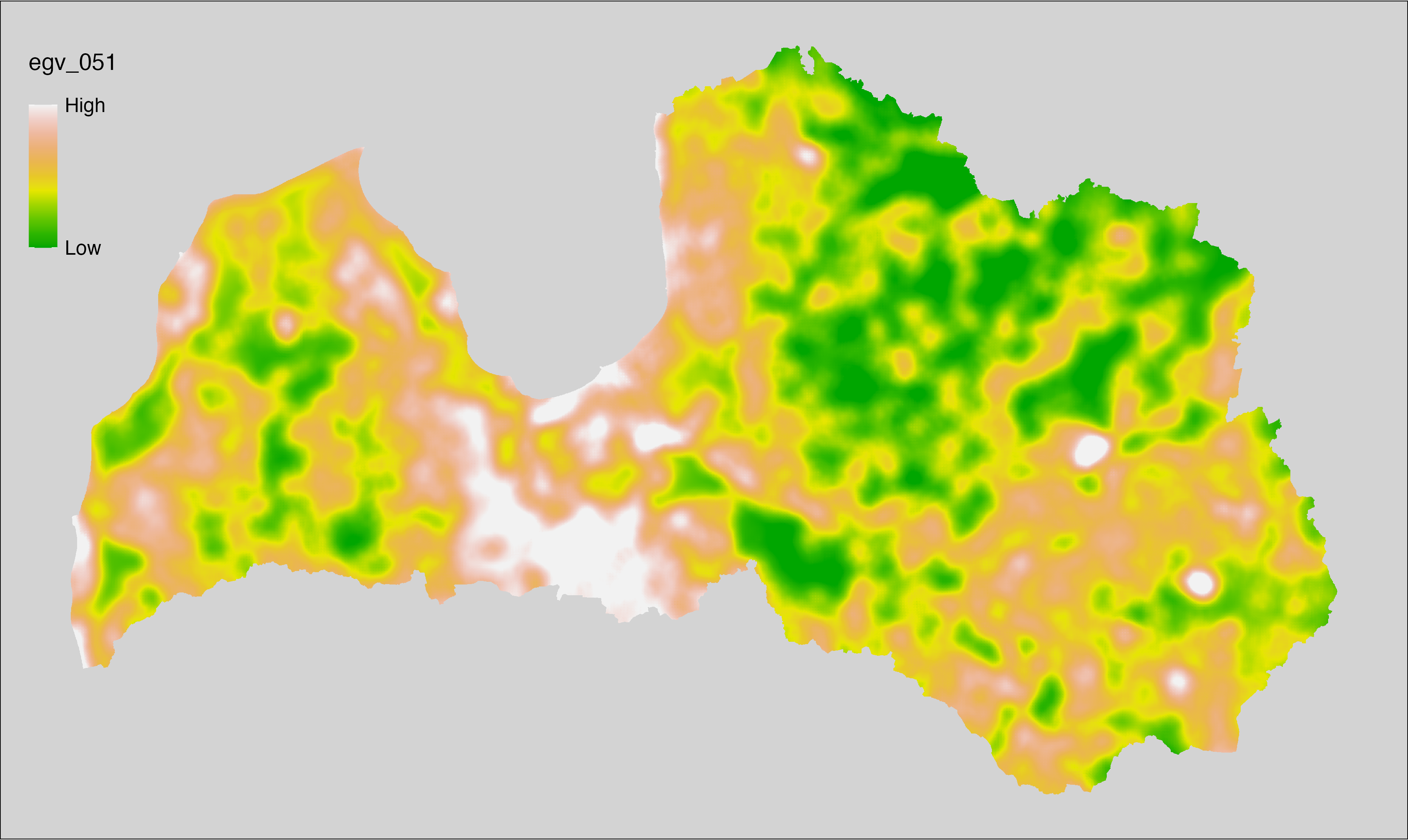
6.52 Climate_CHELSAv2.1-pet-penman-mean_cell
filename: Climate_CHELSAv2.1-pet-penman-mean_cell.tif
layername: egv_052
English name: Mean of monthly mean potential evapotranspiration (kg m⁻² month⁻¹) (CHELSA v2.1) within the analysis cell (1 ha)
Latvian name: Vidējā ik mēneša vidējā potenciālā evapotranspirācija (kg m⁻² month⁻¹) (CHELSA v2.1) analīzes šūnā (1 ha)
Procedure: Directly follows CHELSA v2.1. EGV is prepared using
the workflow egvtools::downscale2egv() with inverse distance weighted (power =
2) gap filling and soft smoothing (power = 0.5) over 5 km radius around each cell.
Finally, the layer is standardised by subtracting the arithmetic mean and
dividing by the root mean squared error.
Code
# libs ----
if(!require(egvtools)) {remotes::install_github("aavotins/egvtools"); require(egvtools)}
# job ----
localname="Climate_CHELSAv2.1-pet-penman-mean_cell.tif"
layername="egv_052"
reading="./Geodata/2024/CHELSA/Climate_CHELSAv2.1-pet-penman-mean_cell.tif"
df <- downscale2egv(
template_path = "./Templates/TemplateRasters/LV100m_10km.tif",
grid_path = "./Templates/TemplateGrids/tikls1km_sauzeme.parquet",
rawfile_path = reading,
out_path = "./RasterGrids_100m/2024/RAW/",
file_name = localname,
layer_name = layername,
fill_gaps = TRUE,
smooth = TRUE,
smooth_radius_km = 5,
plot_result = TRUE)
print(df)
# standardisation ----
if(!require(terra)) {install.packages("terra"); require(terra)}
if(!require(tidyverse)) {install.packages("tidyverse"); require(tidyverse)}
nosaukums="Climate_CHELSAv2.1-pet-penman-mean_cell.tif"
ielasisanas_cels=paste0("./RasterGrids_100m/2024/RAW/",nosaukums)
saglabasanas_cels=paste0("./RasterGrids_100m/2024/Scaled/",nosaukums)
slanis=rast(ielasisanas_cels)
videjais=global(slanis,fun="mean",na.rm=TRUE)
centrets=slanis-videjais[,1]
standartnovirze=terra::global(centrets,fun="rms",na.rm=TRUE)
merogots=centrets/standartnovirze[,1]
writeRaster(merogots,
filename=saglabasanas_cels,
overwrite=TRUE)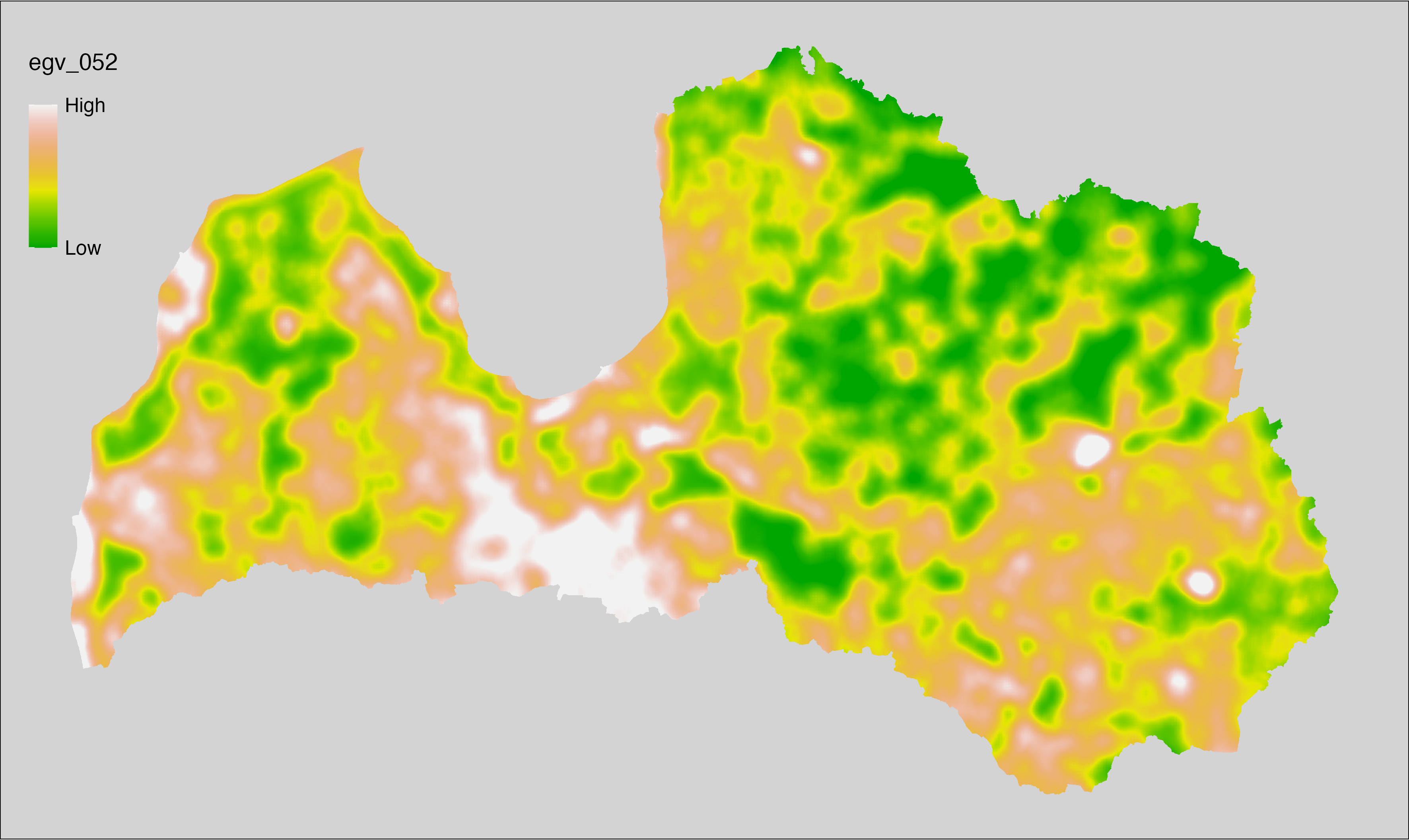
6.53 Climate_CHELSAv2.1-pet-penman-min_cell
filename: Climate_CHELSAv2.1-pet-penman-min_cell.tif
layername: egv_053
English name: Mean of monthly minimum potential evapotranspiration (kg m⁻² month⁻¹) (CHELSA v2.1) within the analysis cell (1 ha)
Latvian name: Vidējā ik mēneša minimālā potenciālā evapotranspirācija (kg m⁻² month⁻¹) (CHELSA v2.1) analīzes šūnā (1 ha)
Procedure: Directly follows CHELSA v2.1. EGV is prepared using
the workflow egvtools::downscale2egv() with inverse distance weighted (power =
2) gap filling and soft smoothing (power = 0.5) over 5 km radius around each cell.
Finally, the layer is standardised by subtracting the arithmetic mean and
dividing by the root mean squared error.
Code
# libs ----
if(!require(egvtools)) {remotes::install_github("aavotins/egvtools"); require(egvtools)}
# job ----
localname="Climate_CHELSAv2.1-pet-penman-min_cell.tif"
layername="egv_053"
reading="./Geodata/2024/CHELSA/Climate_CHELSAv2.1-pet-penman-min_cell.tif"
df <- downscale2egv(
template_path = "./Templates/TemplateRasters/LV100m_10km.tif",
grid_path = "./Templates/TemplateGrids/tikls1km_sauzeme.parquet",
rawfile_path = reading,
out_path = "./RasterGrids_100m/2024/RAW/",
file_name = localname,
layer_name = layername,
fill_gaps = TRUE,
smooth = TRUE,
smooth_radius_km = 5,
plot_result = TRUE)
print(df)
# standardisation ----
if(!require(terra)) {install.packages("terra"); require(terra)}
if(!require(tidyverse)) {install.packages("tidyverse"); require(tidyverse)}
nosaukums="Climate_CHELSAv2.1-pet-penman-min_cell.tif"
ielasisanas_cels=paste0("./RasterGrids_100m/2024/RAW/",nosaukums)
saglabasanas_cels=paste0("./RasterGrids_100m/2024/Scaled/",nosaukums)
slanis=rast(ielasisanas_cels)
videjais=global(slanis,fun="mean",na.rm=TRUE)
centrets=slanis-videjais[,1]
standartnovirze=terra::global(centrets,fun="rms",na.rm=TRUE)
merogots=centrets/standartnovirze[,1]
writeRaster(merogots,
filename=saglabasanas_cels,
overwrite=TRUE)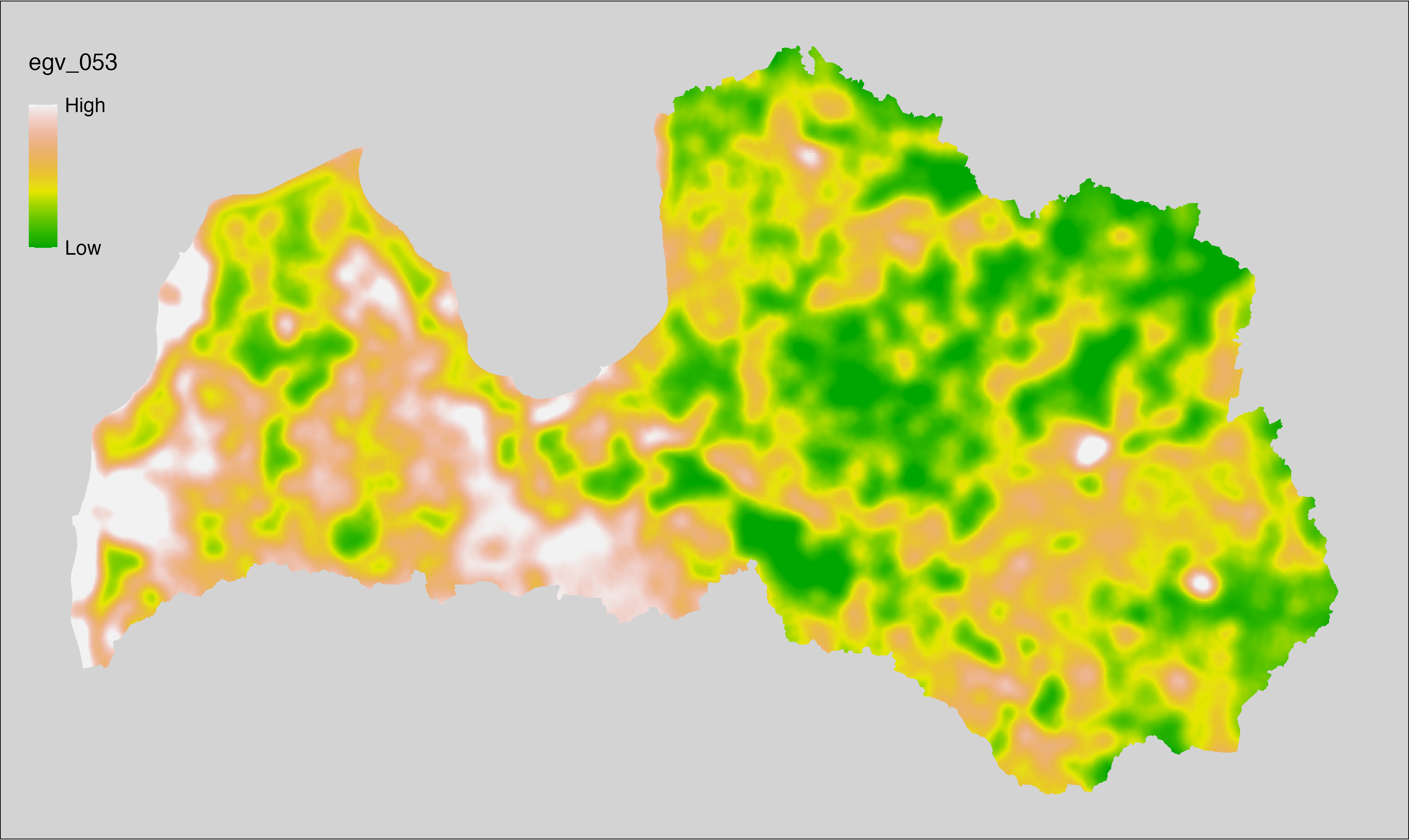
6.54 Climate_CHELSAv2.1-pet-penman-range_cell
filename: Climate_CHELSAv2.1-pet-penman-range_cell.tif
layername: egv_054
English name: Annual range of monthly potential evapotranspiration (kg m⁻² month⁻¹) (CHELSA v2.1) within the analysis cell (1 ha)
Latvian name: Gada potenciālās evapotranspirācijas amplitūda (kg m⁻² month⁻¹) (CHELSA v2.1) analīzes šūnā (1 ha)
Procedure: Directly follows CHELSA v2.1. EGV is prepared using
the workflow egvtools::downscale2egv() with inverse distance weighted (power =
2) gap filling and soft smoothing (power = 0.5) over 5 km radius around each cell.
Finally, the layer is standardised by subtracting the arithmetic mean and
dividing by the root mean squared error.
Code
# libs ----
if(!require(egvtools)) {remotes::install_github("aavotins/egvtools"); require(egvtools)}
# job ----
localname="Climate_CHELSAv2.1-pet-penman-range_cell.tif"
layername="egv_054"
reading="./Geodata/2024/CHELSA/Climate_CHELSAv2.1-pet-penman-range_cell.tif"
df <- downscale2egv(
template_path = "./Templates/TemplateRasters/LV100m_10km.tif",
grid_path = "./Templates/TemplateGrids/tikls1km_sauzeme.parquet",
rawfile_path = reading,
out_path = "./RasterGrids_100m/2024/RAW/",
file_name = localname,
layer_name = layername,
fill_gaps = TRUE,
smooth = TRUE,
smooth_radius_km = 5,
plot_result = TRUE)
print(df)
# standardisation ----
if(!require(terra)) {install.packages("terra"); require(terra)}
if(!require(tidyverse)) {install.packages("tidyverse"); require(tidyverse)}
nosaukums="Climate_CHELSAv2.1-pet-penman-range_cell.tif"
ielasisanas_cels=paste0("./RasterGrids_100m/2024/RAW/",nosaukums)
saglabasanas_cels=paste0("./RasterGrids_100m/2024/Scaled/",nosaukums)
slanis=rast(ielasisanas_cels)
videjais=global(slanis,fun="mean",na.rm=TRUE)
centrets=slanis-videjais[,1]
standartnovirze=terra::global(centrets,fun="rms",na.rm=TRUE)
merogots=centrets/standartnovirze[,1]
writeRaster(merogots,
filename=saglabasanas_cels,
overwrite=TRUE)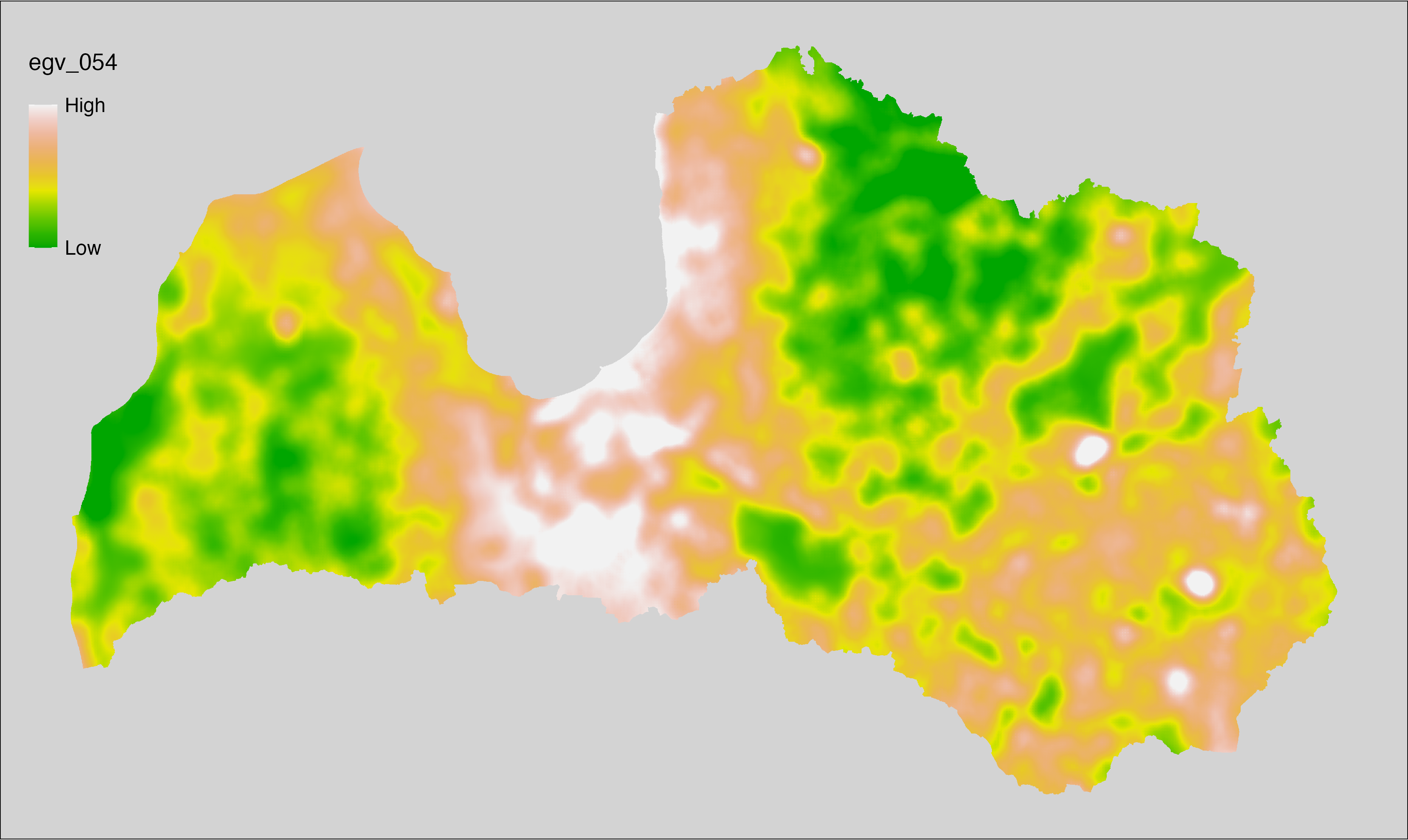
6.55 Climate_CHELSAv2.1-rsds-max_cell
filename: Climate_CHELSAv2.1-rsds-max_cell.tif
layername: egv_055
English name: Mean of monthly maximum surface downwelling shortwave flux in air (MJ m⁻² d⁻¹) (CHELSA v2.1) within the analysis cell (1 ha)
Latvian name: Vidējā ik mēneša maksimālā Zemes virsmu sasniedzošā saules radiācija (MJ m⁻² d⁻¹) (CHELSA v2.1) analīzes šūnā (1 ha)
Procedure: Directly follows CHELSA v2.1. EGV is prepared using
the workflow egvtools::downscale2egv() with inverse distance weighted (power =
2) gap filling and soft smoothing (power = 0.5) over 5 km radius around each cell.
Finally, the layer is standardised by subtracting the arithmetic mean and
dividing by the root mean squared error.
Code
# libs ----
if(!require(egvtools)) {remotes::install_github("aavotins/egvtools"); require(egvtools)}
# job ----
localname="Climate_CHELSAv2.1-rsds-max_cell.tif"
layername="egv_055"
reading="./Geodata/2024/CHELSA/Climate_CHELSAv2.1-rsds-max_cell.tif"
df <- downscale2egv(
template_path = "./Templates/TemplateRasters/LV100m_10km.tif",
grid_path = "./Templates/TemplateGrids/tikls1km_sauzeme.parquet",
rawfile_path = reading,
out_path = "./RasterGrids_100m/2024/RAW/",
file_name = localname,
layer_name = layername,
fill_gaps = TRUE,
smooth = TRUE,
smooth_radius_km = 5,
plot_result = TRUE)
print(df)
# standardisation ----
if(!require(terra)) {install.packages("terra"); require(terra)}
if(!require(tidyverse)) {install.packages("tidyverse"); require(tidyverse)}
nosaukums="Climate_CHELSAv2.1-rsds-max_cell.tif"
ielasisanas_cels=paste0("./RasterGrids_100m/2024/RAW/",nosaukums)
saglabasanas_cels=paste0("./RasterGrids_100m/2024/Scaled/",nosaukums)
slanis=rast(ielasisanas_cels)
videjais=global(slanis,fun="mean",na.rm=TRUE)
centrets=slanis-videjais[,1]
standartnovirze=terra::global(centrets,fun="rms",na.rm=TRUE)
merogots=centrets/standartnovirze[,1]
writeRaster(merogots,
filename=saglabasanas_cels,
overwrite=TRUE)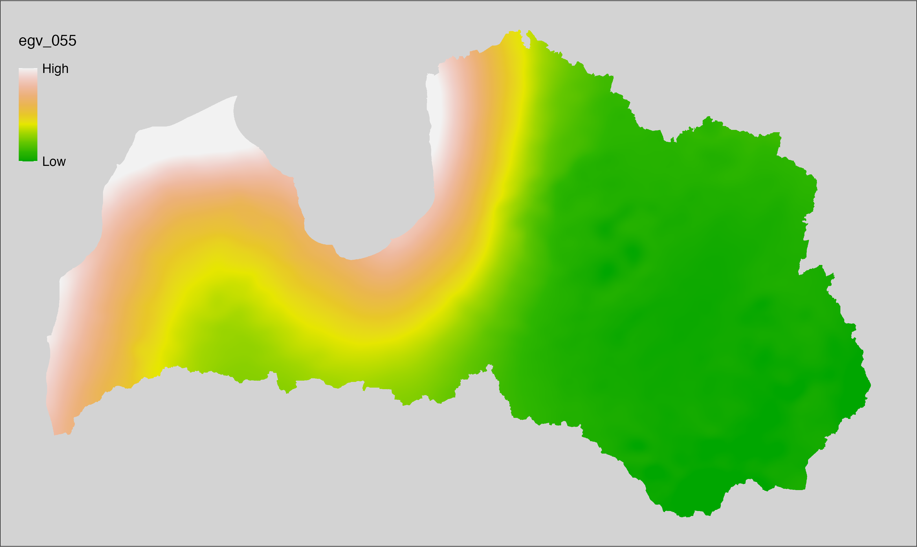
6.56 Climate_CHELSAv2.1-rsds-mean_cell
filename: Climate_CHELSAv2.1-rsds-mean_cell.tif
layername: egv_056
English name: Mean of monthly mean surface downwelling shortwave flux in air (MJ m⁻² d⁻¹) (CHELSA v2.1) within the analysis cell (1 ha)
Latvian name: Vidējā ik mēneša vidējā Zemes virsmu sasniedzošā saules radiācija (MJ m⁻² d⁻¹) (CHELSA v2.1) analīzes šūnā (1 ha)
Procedure: Directly follows CHELSA v2.1. EGV is prepared using
the workflow egvtools::downscale2egv() with inverse distance weighted (power =
2) gap filling and soft smoothing (power = 0.5) over 5 km radius around each cell.
Finally, the layer is standardised by subtracting the arithmetic mean and
dividing by the root mean squared error.
Code
# libs ----
if(!require(egvtools)) {remotes::install_github("aavotins/egvtools"); require(egvtools)}
# job ----
localname="Climate_CHELSAv2.1-rsds-mean_cell.tif"
layername="egv_056"
reading="./Geodata/2024/CHELSA/Climate_CHELSAv2.1-rsds-mean_cell.tif"
df <- downscale2egv(
template_path = "./Templates/TemplateRasters/LV100m_10km.tif",
grid_path = "./Templates/TemplateGrids/tikls1km_sauzeme.parquet",
rawfile_path = reading,
out_path = "./RasterGrids_100m/2024/RAW/",
file_name = localname,
layer_name = layername,
fill_gaps = TRUE,
smooth = TRUE,
smooth_radius_km = 5,
plot_result = TRUE)
print(df)
# standardisation ----
if(!require(terra)) {install.packages("terra"); require(terra)}
if(!require(tidyverse)) {install.packages("tidyverse"); require(tidyverse)}
nosaukums="Climate_CHELSAv2.1-rsds-mean_cell.tif"
ielasisanas_cels=paste0("./RasterGrids_100m/2024/RAW/",nosaukums)
saglabasanas_cels=paste0("./RasterGrids_100m/2024/Scaled/",nosaukums)
slanis=rast(ielasisanas_cels)
videjais=global(slanis,fun="mean",na.rm=TRUE)
centrets=slanis-videjais[,1]
standartnovirze=terra::global(centrets,fun="rms",na.rm=TRUE)
merogots=centrets/standartnovirze[,1]
writeRaster(merogots,
filename=saglabasanas_cels,
overwrite=TRUE)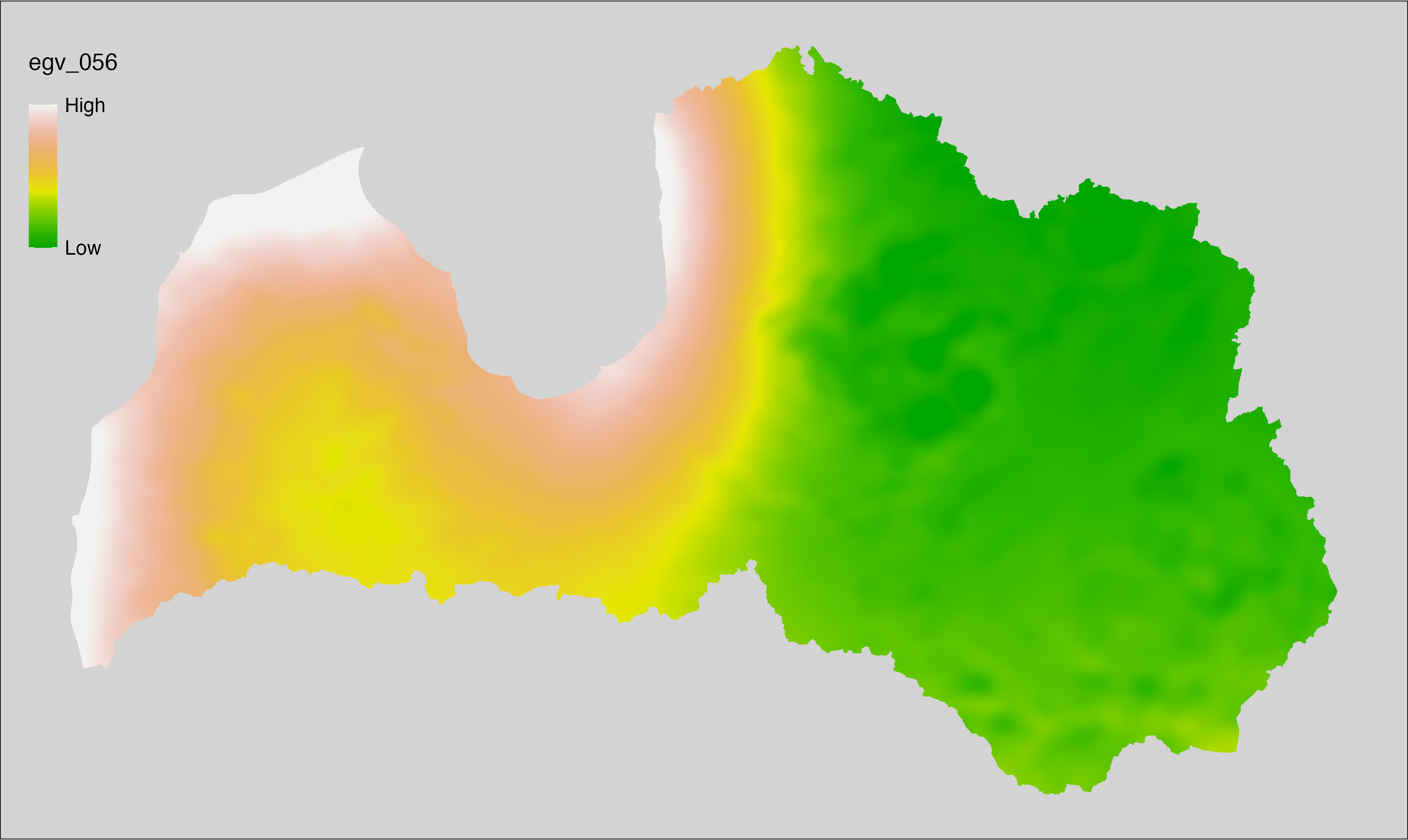
6.57 Climate_CHELSAv2.1-rsds-min_cell
filename: Climate_CHELSAv2.1-rsds-min_cell.tif
layername: egv_057
English name: Mean of monthly minimum surface shortwave flux in air (MJ m⁻² d⁻¹) (CHELSA v2.1) within the analysis cell (1 ha)
Latvian name: Vidējā ik mēneša minimālā Zemes virsmu sasniedzošā saules radiācija (MJ m⁻² d⁻¹) (CHELSA v2.1) analīzes šūnā (1 ha)
Procedure: Directly follows CHELSA v2.1. EGV is prepared using
the workflow egvtools::downscale2egv() with inverse distance weighted (power =
2) gap filling and soft smoothing (power = 0.5) over 5 km radius around each cell.
Finally, the layer is standardised by subtracting the arithmetic mean and
dividing by the root mean squared error.
Code
# libs ----
if(!require(egvtools)) {remotes::install_github("aavotins/egvtools"); require(egvtools)}
# job ----
localname="Climate_CHELSAv2.1-rsds-min_cell.tif"
layername="egv_057"
reading="./Geodata/2024/CHELSA/Climate_CHELSAv2.1-rsds-min_cell.tif"
df <- downscale2egv(
template_path = "./Templates/TemplateRasters/LV100m_10km.tif",
grid_path = "./Templates/TemplateGrids/tikls1km_sauzeme.parquet",
rawfile_path = reading,
out_path = "./RasterGrids_100m/2024/RAW/",
file_name = localname,
layer_name = layername,
fill_gaps = TRUE,
smooth = TRUE,
smooth_radius_km = 5,
plot_result = TRUE)
print(df)
# standardisation ----
if(!require(terra)) {install.packages("terra"); require(terra)}
if(!require(tidyverse)) {install.packages("tidyverse"); require(tidyverse)}
nosaukums="Climate_CHELSAv2.1-rsds-min_cell.tif"
ielasisanas_cels=paste0("./RasterGrids_100m/2024/RAW/",nosaukums)
saglabasanas_cels=paste0("./RasterGrids_100m/2024/Scaled/",nosaukums)
slanis=rast(ielasisanas_cels)
videjais=global(slanis,fun="mean",na.rm=TRUE)
centrets=slanis-videjais[,1]
standartnovirze=terra::global(centrets,fun="rms",na.rm=TRUE)
merogots=centrets/standartnovirze[,1]
writeRaster(merogots,
filename=saglabasanas_cels,
overwrite=TRUE)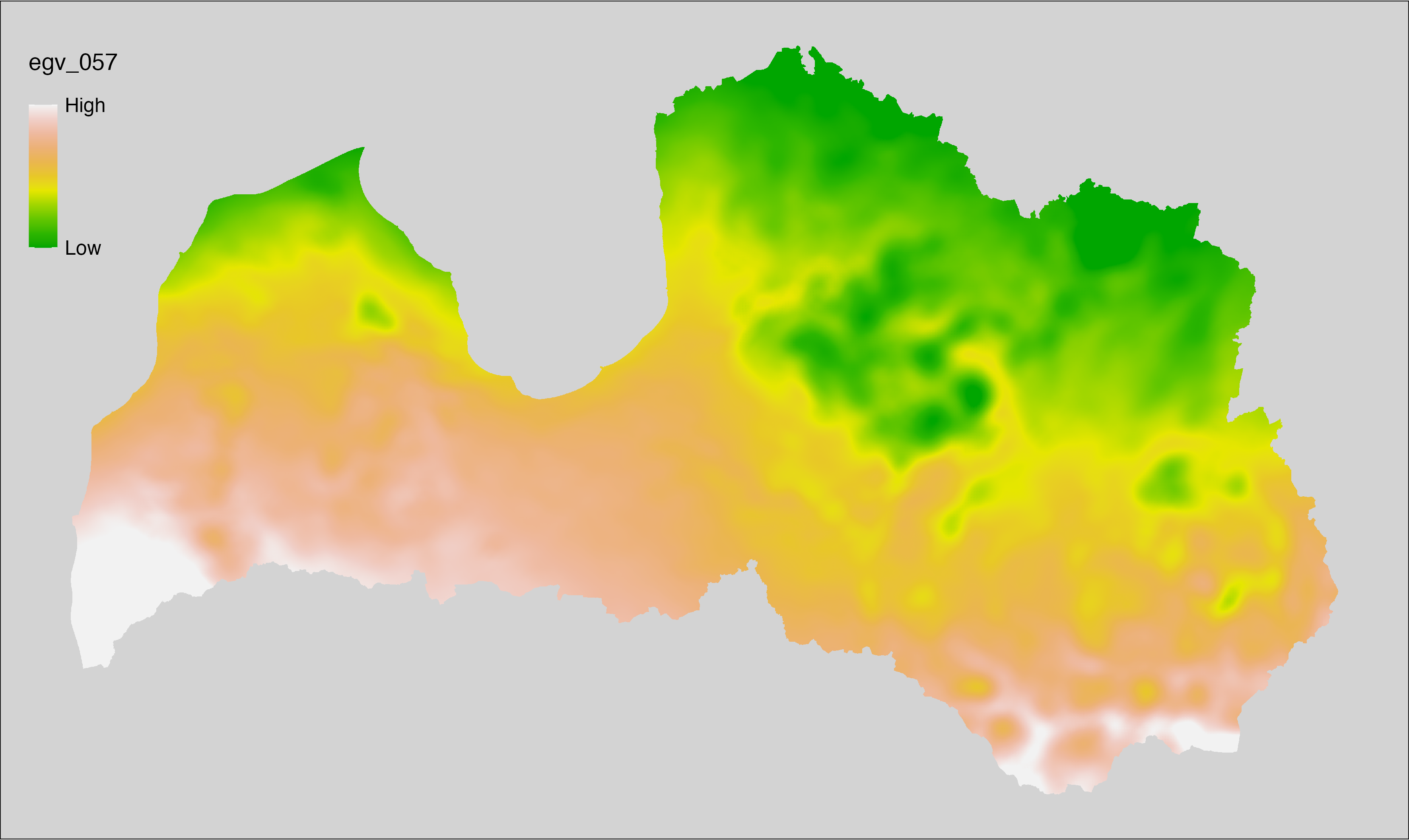
6.58 Climate_CHELSAv2.1-rsds-range_cell
filename: Climate_CHELSAv2.1-rsds-range_cell.tif
layername: egv_058
English name: Annual range of daily mean surface downwelling shortwave flux in air (MJ m⁻² d⁻¹) (CHELSA v2.1) within the analysis cell (1 ha)
Latvian name: Gada amplitūda ik dienas vidējai Zemes virsmu sasniedzošajai saules radiācijai (MJ m⁻² d⁻¹) (CHELSA v2.1) analīzes šūnā (1 ha)
Procedure: Directly follows CHELSA v2.1. EGV is prepared using
the workflow egvtools::downscale2egv() with inverse distance weighted (power =
2) gap filling and soft smoothing (power = 0.5) over 5 km radius around each cell.
Finally, the layer is standardised by subtracting the arithmetic mean and
dividing by the root mean squared error.
Code
# libs ----
if(!require(egvtools)) {remotes::install_github("aavotins/egvtools"); require(egvtools)}
# job ----
localname="Climate_CHELSAv2.1-rsds-range_cell.tif"
layername="egv_058"
reading="./Geodata/2024/CHELSA/Climate_CHELSAv2.1-rsds-range_cell.tif"
df <- downscale2egv(
template_path = "./Templates/TemplateRasters/LV100m_10km.tif",
grid_path = "./Templates/TemplateGrids/tikls1km_sauzeme.parquet",
rawfile_path = reading,
out_path = "./RasterGrids_100m/2024/RAW/",
file_name = localname,
layer_name = layername,
fill_gaps = TRUE,
smooth = TRUE,
smooth_radius_km = 5,
plot_result = TRUE)
print(df)
# standardisation ----
if(!require(terra)) {install.packages("terra"); require(terra)}
if(!require(tidyverse)) {install.packages("tidyverse"); require(tidyverse)}
nosaukums="Climate_CHELSAv2.1-rsds-range_cell.tif"
ielasisanas_cels=paste0("./RasterGrids_100m/2024/RAW/",nosaukums)
saglabasanas_cels=paste0("./RasterGrids_100m/2024/Scaled/",nosaukums)
slanis=rast(ielasisanas_cels)
videjais=global(slanis,fun="mean",na.rm=TRUE)
centrets=slanis-videjais[,1]
standartnovirze=terra::global(centrets,fun="rms",na.rm=TRUE)
merogots=centrets/standartnovirze[,1]
writeRaster(merogots,
filename=saglabasanas_cels,
overwrite=TRUE)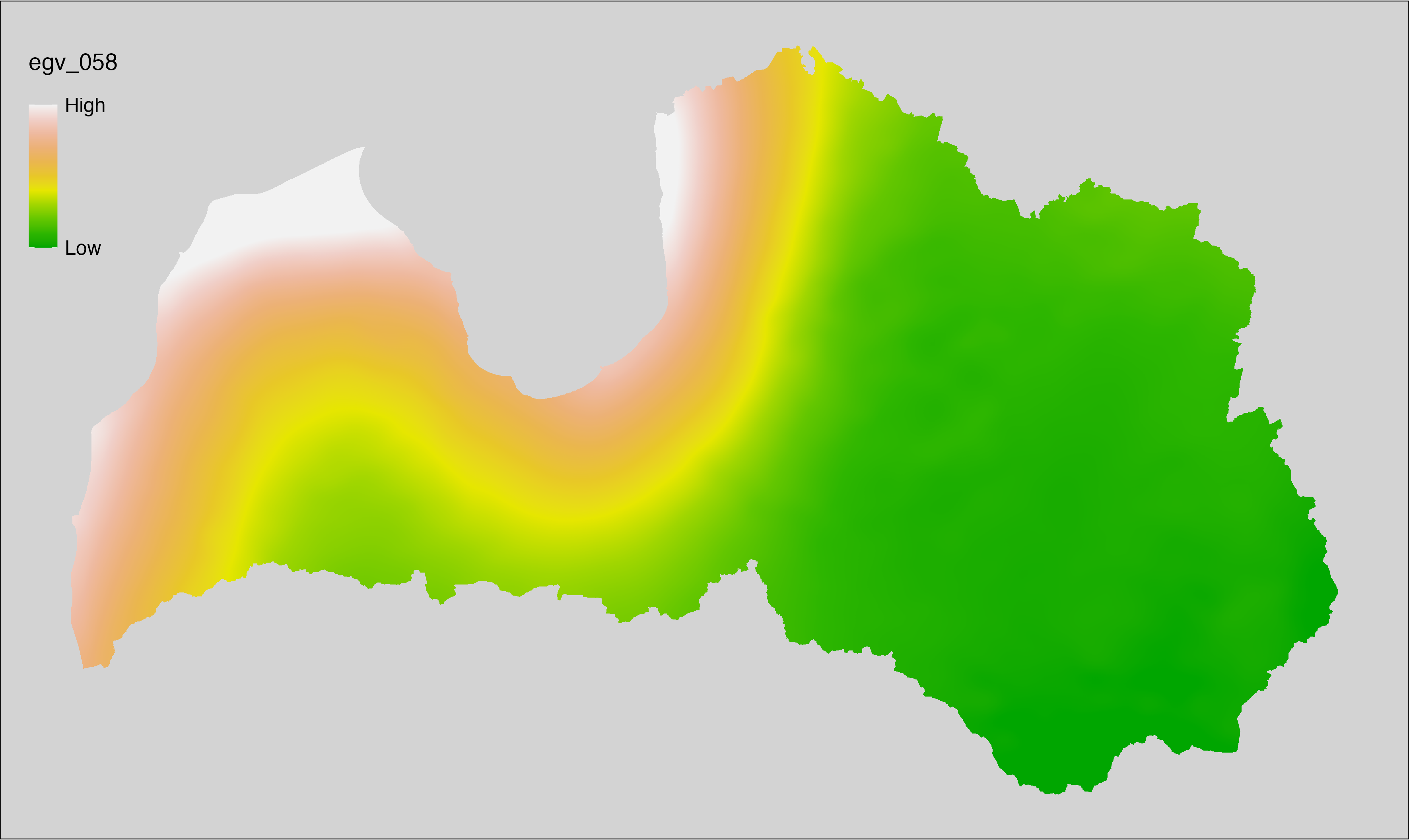
6.59 Climate_CHELSAv2.1-scd_cell
filename: Climate_CHELSAv2.1-scd_cell.tif
layername: egv_059
English name: Number of days with snow cover (TREELIM) (CHELSA v2.1) within the analysis cell (1 ha)
Latvian name: Dienu ar sniega segu skaits (TREELIM) (CHELSA v2.1) analīzes šūnā (1 ha)
Procedure: Directly follows CHELSA v2.1. EGV is prepared using
the workflow egvtools::downscale2egv() with inverse distance weighted (power =
2) gap filling and soft smoothing (power = 0.5) over 5 km radius around each cell.
Finally, the layer is standardised by subtracting the arithmetic mean and
dividing by the root mean squared error.
Code
# libs ----
if(!require(egvtools)) {remotes::install_github("aavotins/egvtools"); require(egvtools)}
# job ----
localname="Climate_CHELSAv2.1-scd_cell.tif"
layername="egv_059"
reading="./Geodata/2024/CHELSA/Climate_CHELSAv2.1-scd_cell.tif"
df <- downscale2egv(
template_path = "./Templates/TemplateRasters/LV100m_10km.tif",
grid_path = "./Templates/TemplateGrids/tikls1km_sauzeme.parquet",
rawfile_path = reading,
out_path = "./RasterGrids_100m/2024/RAW/",
file_name = localname,
layer_name = layername,
fill_gaps = TRUE,
smooth = TRUE,
smooth_radius_km = 5,
plot_result = TRUE)
print(df)
# standardisation ----
if(!require(terra)) {install.packages("terra"); require(terra)}
if(!require(tidyverse)) {install.packages("tidyverse"); require(tidyverse)}
nosaukums="Climate_CHELSAv2.1-scd_cell.tif"
ielasisanas_cels=paste0("./RasterGrids_100m/2024/RAW/",nosaukums)
saglabasanas_cels=paste0("./RasterGrids_100m/2024/Scaled/",nosaukums)
slanis=rast(ielasisanas_cels)
videjais=global(slanis,fun="mean",na.rm=TRUE)
centrets=slanis-videjais[,1]
standartnovirze=terra::global(centrets,fun="rms",na.rm=TRUE)
merogots=centrets/standartnovirze[,1]
writeRaster(merogots,
filename=saglabasanas_cels,
overwrite=TRUE)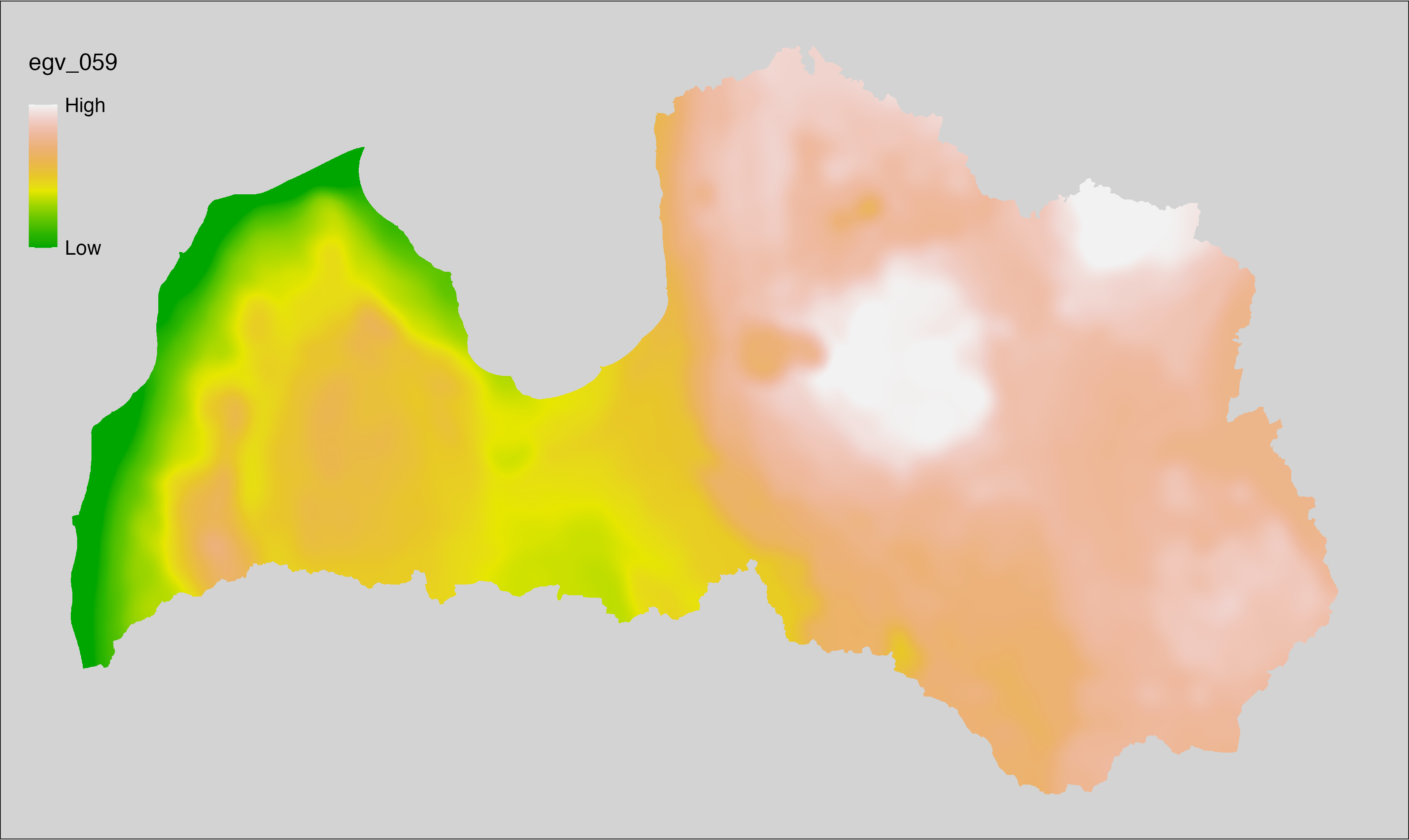
6.60 Climate_CHELSAv2.1-sfcWind-max_cell
filename: Climate_CHELSAv2.1-sfcWind-max_cell.tif
layername: egv_060
English name: Mean of monthly maximum near-surface wind speed (m s⁻¹) (CHELSA v2.1) within the analysis cell (1 ha)
Latvian name: Vidējais ik mēneša maksimālais piezemes slāņa vēja ātrums (m s⁻¹) (CHELSA v2.1) analīzes šūnā (1 ha)
Procedure: Directly follows CHELSA v2.1. EGV is prepared using
the workflow egvtools::downscale2egv() with inverse distance weighted (power =
2) gap filling and soft smoothing (power = 0.5) over 5 km radius around each cell.
Finally, the layer is standardised by subtracting the arithmetic mean and
dividing by the root mean squared error.
Code
# libs ----
if(!require(egvtools)) {remotes::install_github("aavotins/egvtools"); require(egvtools)}
# job ----
localname="Climate_CHELSAv2.1-sfcWind-max_cell.tif"
layername="egv_060"
reading="./Geodata/2024/CHELSA/Climate_CHELSAv2.1-sfcWind-max_cell.tif"
df <- downscale2egv(
template_path = "./Templates/TemplateRasters/LV100m_10km.tif",
grid_path = "./Templates/TemplateGrids/tikls1km_sauzeme.parquet",
rawfile_path = reading,
out_path = "./RasterGrids_100m/2024/RAW/",
file_name = localname,
layer_name = layername,
fill_gaps = TRUE,
smooth = TRUE,
smooth_radius_km = 5,
plot_result = TRUE)
print(df)
# standardisation ----
if(!require(terra)) {install.packages("terra"); require(terra)}
if(!require(tidyverse)) {install.packages("tidyverse"); require(tidyverse)}
nosaukums="Climate_CHELSAv2.1-sfcWind-max_cell.tif"
ielasisanas_cels=paste0("./RasterGrids_100m/2024/RAW/",nosaukums)
saglabasanas_cels=paste0("./RasterGrids_100m/2024/Scaled/",nosaukums)
slanis=rast(ielasisanas_cels)
videjais=global(slanis,fun="mean",na.rm=TRUE)
centrets=slanis-videjais[,1]
standartnovirze=terra::global(centrets,fun="rms",na.rm=TRUE)
merogots=centrets/standartnovirze[,1]
writeRaster(merogots,
filename=saglabasanas_cels,
overwrite=TRUE)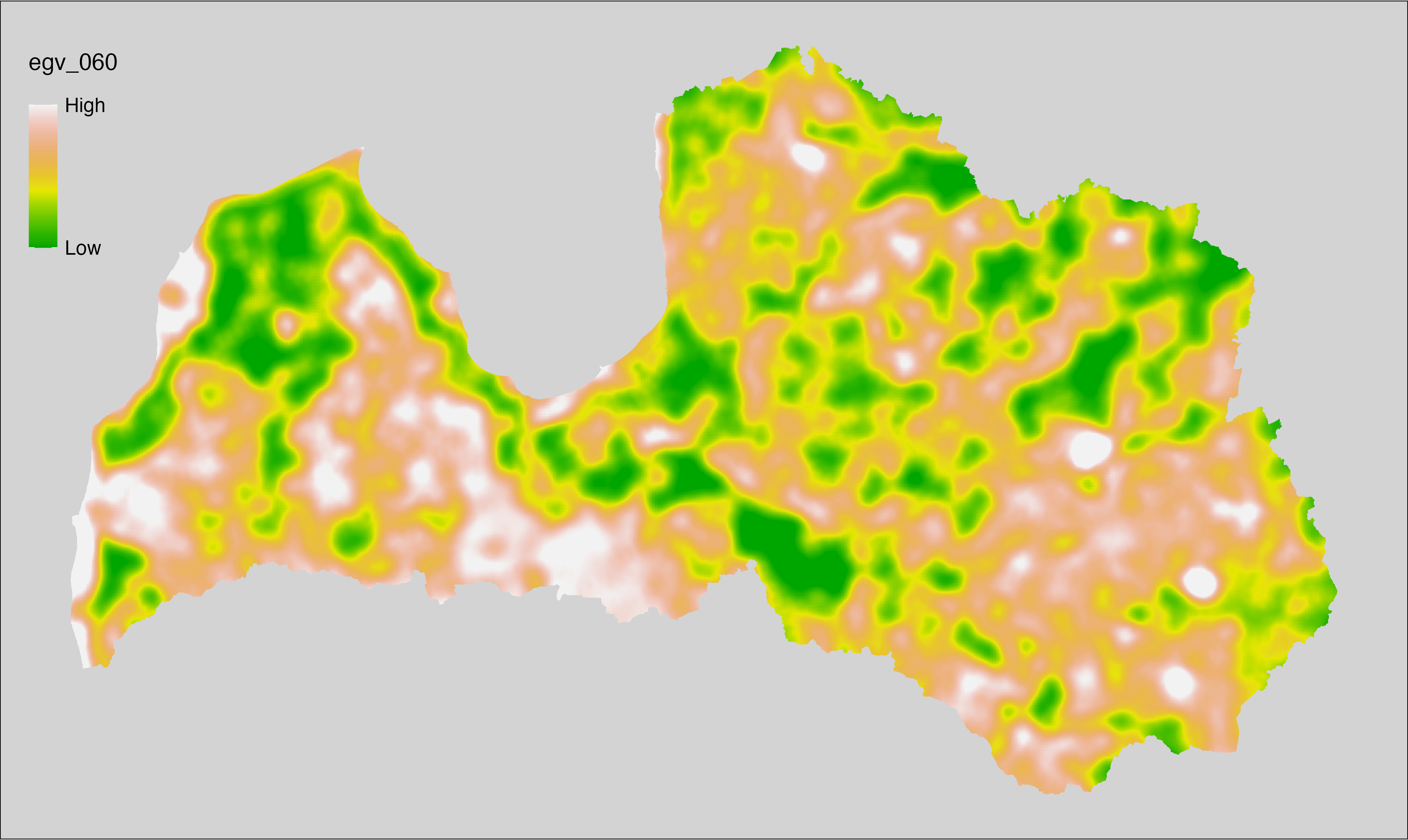
6.61 Climate_CHELSAv2.1-sfcWind-mean_cell
filename: Climate_CHELSAv2.1-sfcWind-mean_cell.tif
layername: egv_061
English name: Mean of monthly mean near-surface wind speed (m s⁻¹) (CHELSA v2.1) within the analysis cell (1 ha)
Latvian name: Vidējais ik mēneša vidējais piezemes slāņa vēja ātrums (m s⁻¹) (CHELSA v2.1) analīzes šūnā (1 ha)
Procedure: Directly follows CHELSA v2.1. EGV is prepared using
the workflow egvtools::downscale2egv() with inverse distance weighted (power =
2) gap filling and soft smoothing (power = 0.5) over 5 km radius around each cell.
Finally, the layer is standardised by subtracting the arithmetic mean and
dividing by the root mean squared error.
Code
# libs ----
if(!require(egvtools)) {remotes::install_github("aavotins/egvtools"); require(egvtools)}
# job ----
localname="Climate_CHELSAv2.1-sfcWind-mean_cell.tif"
layername="egv_061"
reading="./Geodata/2024/CHELSA/Climate_CHELSAv2.1-sfcWind-mean_cell.tif"
df <- downscale2egv(
template_path = "./Templates/TemplateRasters/LV100m_10km.tif",
grid_path = "./Templates/TemplateGrids/tikls1km_sauzeme.parquet",
rawfile_path = reading,
out_path = "./RasterGrids_100m/2024/RAW/",
file_name = localname,
layer_name = layername,
fill_gaps = TRUE,
smooth = TRUE,
smooth_radius_km = 5,
plot_result = TRUE)
print(df)
# standardisation ----
if(!require(terra)) {install.packages("terra"); require(terra)}
if(!require(tidyverse)) {install.packages("tidyverse"); require(tidyverse)}
nosaukums="Climate_CHELSAv2.1-sfcWind-mean_cell.tif"
ielasisanas_cels=paste0("./RasterGrids_100m/2024/RAW/",nosaukums)
saglabasanas_cels=paste0("./RasterGrids_100m/2024/Scaled/",nosaukums)
slanis=rast(ielasisanas_cels)
videjais=global(slanis,fun="mean",na.rm=TRUE)
centrets=slanis-videjais[,1]
standartnovirze=terra::global(centrets,fun="rms",na.rm=TRUE)
merogots=centrets/standartnovirze[,1]
writeRaster(merogots,
filename=saglabasanas_cels,
overwrite=TRUE)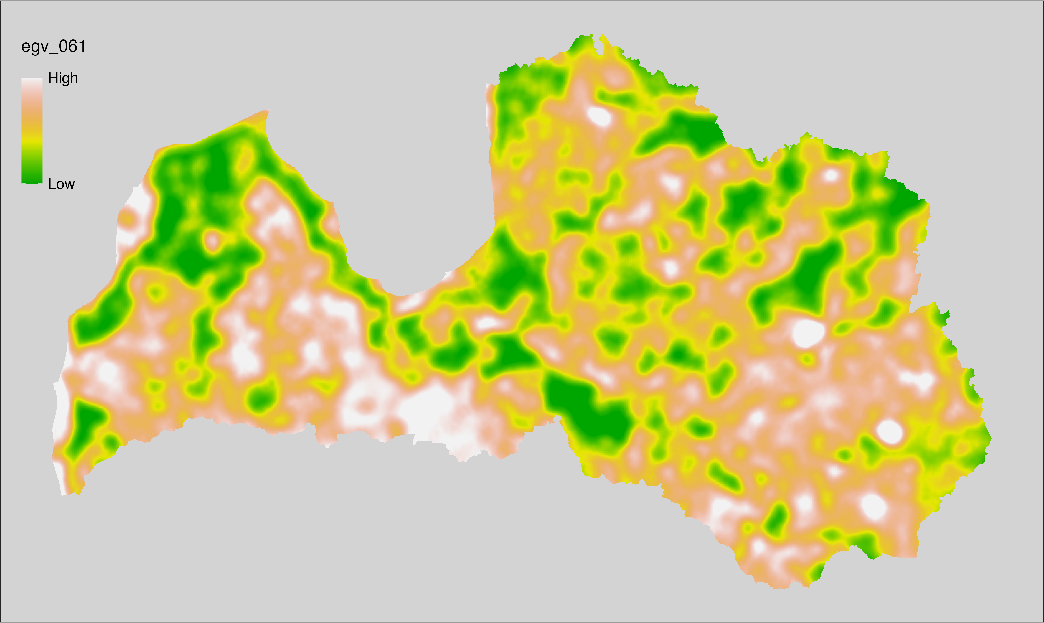
6.62 Climate_CHELSAv2.1-sfcWind-min_cell
filename: Climate_CHELSAv2.1-sfcWind-min_cell.tif
layername: egv_062
English name: Mean of monthly minimum near-surface wind speed (m s⁻¹) (CHELSA v2.1) within the analysis cell (1 ha)
Latvian name: Vidējais ik mēneša minimālais piezemes slāņa vēja ātrums (m s⁻¹) (CHELSA v2.1) analīzes šūnā (1 ha)
Procedure: Directly follows CHELSA v2.1. EGV is prepared using
the workflow egvtools::downscale2egv() with inverse distance weighted (power =
2) gap filling and soft smoothing (power = 0.5) over 5 km radius around each cell.
Finally, the layer is standardised by subtracting the arithmetic mean and
dividing by the root mean squared error.
Code
# libs ----
if(!require(egvtools)) {remotes::install_github("aavotins/egvtools"); require(egvtools)}
# job ----
localname="Climate_CHELSAv2.1-sfcWind-min_cell.tif"
layername="egv_062"
reading="./Geodata/2024/CHELSA/Climate_CHELSAv2.1-sfcWind-min_cell.tif"
df <- downscale2egv(
template_path = "./Templates/TemplateRasters/LV100m_10km.tif",
grid_path = "./Templates/TemplateGrids/tikls1km_sauzeme.parquet",
rawfile_path = reading,
out_path = "./RasterGrids_100m/2024/RAW/",
file_name = localname,
layer_name = layername,
fill_gaps = TRUE,
smooth = TRUE,
smooth_radius_km = 5,
plot_result = TRUE)
print(df)
# standardisation ----
if(!require(terra)) {install.packages("terra"); require(terra)}
if(!require(tidyverse)) {install.packages("tidyverse"); require(tidyverse)}
nosaukums="Climate_CHELSAv2.1-sfcWind-min_cell.tif"
ielasisanas_cels=paste0("./RasterGrids_100m/2024/RAW/",nosaukums)
saglabasanas_cels=paste0("./RasterGrids_100m/2024/Scaled/",nosaukums)
slanis=rast(ielasisanas_cels)
videjais=global(slanis,fun="mean",na.rm=TRUE)
centrets=slanis-videjais[,1]
standartnovirze=terra::global(centrets,fun="rms",na.rm=TRUE)
merogots=centrets/standartnovirze[,1]
writeRaster(merogots,
filename=saglabasanas_cels,
overwrite=TRUE)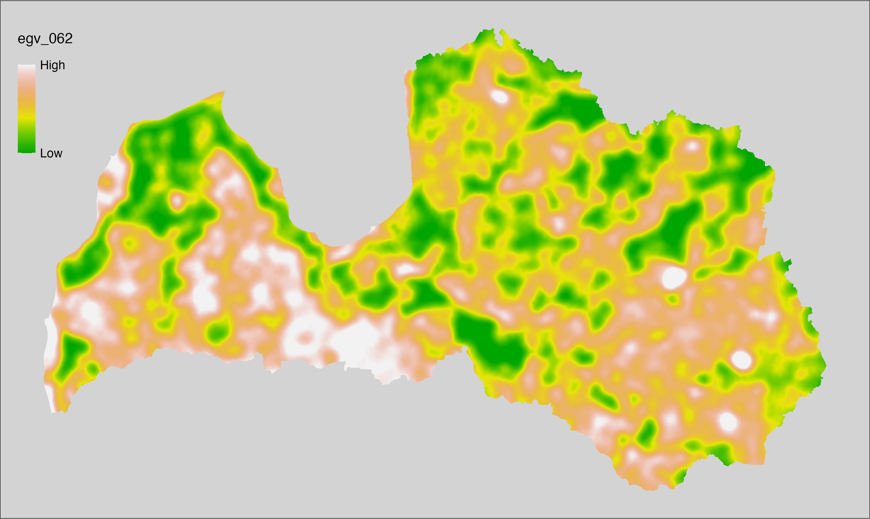
6.63 Climate_CHELSAv2.1-sfcWind-range_cell
filename: Climate_CHELSAv2.1-sfcWind-range_cell.tif
layername: egv_063
English name: Annual range of monthly mean near-surface wind speed (m s⁻¹) (CHELSA v2.1) within the analysis cell (1 ha)
Latvian name: Gada amplitūda ik mēneša vidējam piezemes slāņa vēja ātrumam (m s⁻¹) (CHELSA v2.1) analīzes šūnā (1 ha)
Procedure: Directly follows CHELSA v2.1. EGV is prepared using
the workflow egvtools::downscale2egv() with inverse distance weighted (power =
2) gap filling and soft smoothing (power = 0.5) over 5 km radius around each cell.
Finally, the layer is standardised by subtracting the arithmetic mean and
dividing by the root mean squared error.
Code
# libs ----
if(!require(egvtools)) {remotes::install_github("aavotins/egvtools"); require(egvtools)}
# job ----
localname="Climate_CHELSAv2.1-sfcWind-range_cell.tif"
layername="egv_063"
reading="./Geodata/2024/CHELSA/Climate_CHELSAv2.1-sfcWind-range_cell.tif"
df <- downscale2egv(
template_path = "./Templates/TemplateRasters/LV100m_10km.tif",
grid_path = "./Templates/TemplateGrids/tikls1km_sauzeme.parquet",
rawfile_path = reading,
out_path = "./RasterGrids_100m/2024/RAW/",
file_name = localname,
layer_name = layername,
fill_gaps = TRUE,
smooth = TRUE,
smooth_radius_km = 5,
plot_result = TRUE)
print(df)
# standardisation ----
if(!require(terra)) {install.packages("terra"); require(terra)}
if(!require(tidyverse)) {install.packages("tidyverse"); require(tidyverse)}
nosaukums="Climate_CHELSAv2.1-sfcWind-range_cell.tif"
ielasisanas_cels=paste0("./RasterGrids_100m/2024/RAW/",nosaukums)
saglabasanas_cels=paste0("./RasterGrids_100m/2024/Scaled/",nosaukums)
slanis=rast(ielasisanas_cels)
videjais=global(slanis,fun="mean",na.rm=TRUE)
centrets=slanis-videjais[,1]
standartnovirze=terra::global(centrets,fun="rms",na.rm=TRUE)
merogots=centrets/standartnovirze[,1]
writeRaster(merogots,
filename=saglabasanas_cels,
overwrite=TRUE)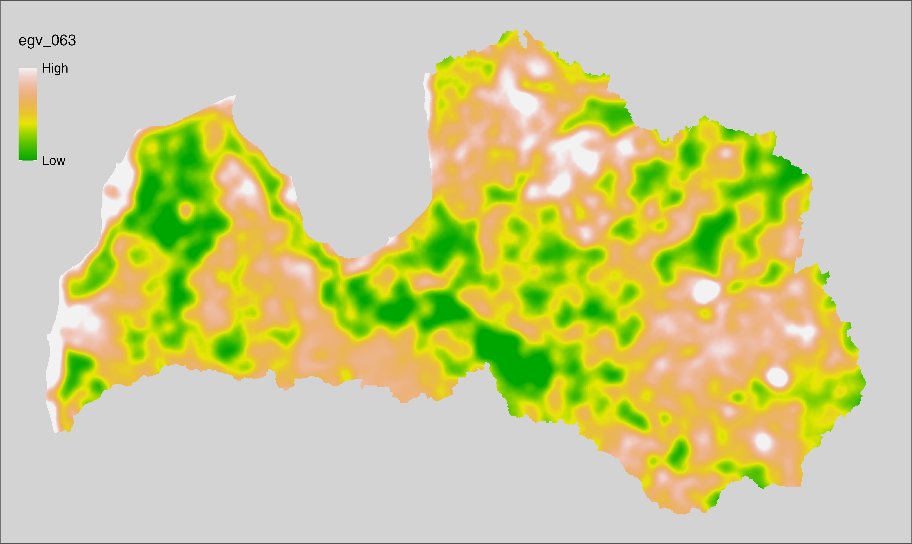
6.64 Climate_CHELSAv2.1-swb_cell
filename: Climate_CHELSAv2.1-swb_cell.tif
layername: egv_064
English name: Site water balance (kg m⁻² year⁻¹) (CHELSA v2.1) within the analysis cell (1 ha)
Latvian name: Ūdens bilance (kg m⁻² year⁻¹) (CHELSA v2.1) analīzes šūnā (1 ha)
Procedure: Directly follows CHELSA v2.1. EGV is prepared using
the workflow egvtools::downscale2egv() with inverse distance weighted (power =
2) gap filling and soft smoothing (power = 0.5) over 5 km radius around each cell.
Finally, the layer is standardised by subtracting the arithmetic mean and
dividing by the root mean squared error.
Code
# libs ----
if(!require(egvtools)) {remotes::install_github("aavotins/egvtools"); require(egvtools)}
# job ----
localname="Climate_CHELSAv2.1-swb_cell.tif"
layername="egv_064"
reading="./Geodata/2024/CHELSA/Climate_CHELSAv2.1-swb_cell.tif"
df <- downscale2egv(
template_path = "./Templates/TemplateRasters/LV100m_10km.tif",
grid_path = "./Templates/TemplateGrids/tikls1km_sauzeme.parquet",
rawfile_path = reading,
out_path = "./RasterGrids_100m/2024/RAW/",
file_name = localname,
layer_name = layername,
fill_gaps = TRUE,
smooth = TRUE,
smooth_radius_km = 5,
plot_result = TRUE)
print(df)
# standardisation ----
if(!require(terra)) {install.packages("terra"); require(terra)}
if(!require(tidyverse)) {install.packages("tidyverse"); require(tidyverse)}
nosaukums="Climate_CHELSAv2.1-swb_cell.tif"
ielasisanas_cels=paste0("./RasterGrids_100m/2024/RAW/",nosaukums)
saglabasanas_cels=paste0("./RasterGrids_100m/2024/Scaled/",nosaukums)
slanis=rast(ielasisanas_cels)
videjais=global(slanis,fun="mean",na.rm=TRUE)
centrets=slanis-videjais[,1]
standartnovirze=terra::global(centrets,fun="rms",na.rm=TRUE)
merogots=centrets/standartnovirze[,1]
writeRaster(merogots,
filename=saglabasanas_cels,
overwrite=TRUE)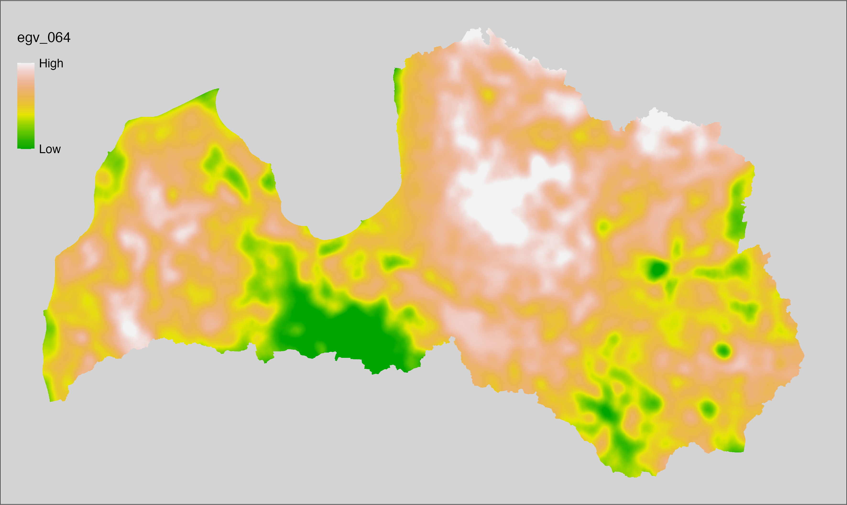
6.65 Climate_CHELSAv2.1-swe_cell
filename: Climate_CHELSAv2.1-swe_cell.tif
layername: egv_065
English name: Snow water equivalent (kg m⁻² year⁻¹) (CHELSA v2.1) within the analysis cell (1 ha)
Latvian name: Ūdens ekvivalents sniegā (kg m⁻² year⁻¹) (CHELSA v2.1) analīzes šūnā (1 ha)
Procedure: Directly follows CHELSA v2.1. EGV is prepared using
the workflow egvtools::downscale2egv() with inverse distance weighted (power =
2) gap filling and soft smoothing (power = 0.5) over 5 km radius around each cell.
Finally, the layer is standardised by subtracting the arithmetic mean and
dividing by the root mean squared error.
Code
# libs ----
if(!require(egvtools)) {remotes::install_github("aavotins/egvtools"); require(egvtools)}
# job ----
localname="Climate_CHELSAv2.1-swe_cell.tif"
layername="egv_065"
reading="./Geodata/2024/CHELSA/Climate_CHELSAv2.1-swe_cell.tif"
df <- downscale2egv(
template_path = "./Templates/TemplateRasters/LV100m_10km.tif",
grid_path = "./Templates/TemplateGrids/tikls1km_sauzeme.parquet",
rawfile_path = reading,
out_path = "./RasterGrids_100m/2024/RAW/",
file_name = localname,
layer_name = layername,
fill_gaps = TRUE,
smooth = TRUE,
smooth_radius_km = 5,
plot_result = TRUE)
print(df)
# standardisation ----
if(!require(terra)) {install.packages("terra"); require(terra)}
if(!require(tidyverse)) {install.packages("tidyverse"); require(tidyverse)}
nosaukums="Climate_CHELSAv2.1-swe_cell.tif"
ielasisanas_cels=paste0("./RasterGrids_100m/2024/RAW/",nosaukums)
saglabasanas_cels=paste0("./RasterGrids_100m/2024/Scaled/",nosaukums)
slanis=rast(ielasisanas_cels)
videjais=global(slanis,fun="mean",na.rm=TRUE)
centrets=slanis-videjais[,1]
standartnovirze=terra::global(centrets,fun="rms",na.rm=TRUE)
merogots=centrets/standartnovirze[,1]
writeRaster(merogots,
filename=saglabasanas_cels,
overwrite=TRUE)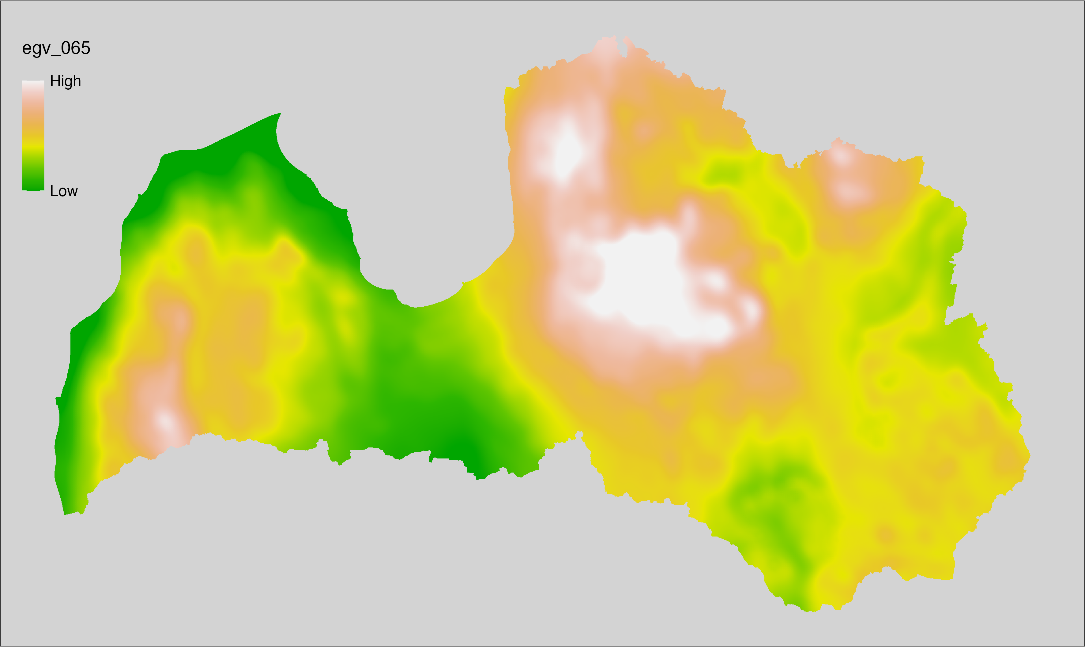
6.66 Climate_CHELSAv2.1-vpd-max_cell
filename: Climate_CHELSAv2.1-vpd-max_cell.tif
layername: egv_066
English name: Mean of monthly maximum vapor pressure deficit (Pa) (CHELSA v2.1) within the analysis cell (1 ha)
Latvian name: Vidējais ik mēneša maksimālais iztvaikošanas spiediena deficīts (Pa) (CHELSA v2.1) analīzes šūnā (1 ha)
Procedure: Directly follows CHELSA v2.1. EGV is prepared using
the workflow egvtools::downscale2egv() with inverse distance weighted (power =
2) gap filling and soft smoothing (power = 0.5) over 5 km radius around each cell.
Finally, the layer is standardised by subtracting the arithmetic mean and
dividing by the root mean squared error.
Code
# libs ----
if(!require(egvtools)) {remotes::install_github("aavotins/egvtools"); require(egvtools)}
# job ----
localname="Climate_CHELSAv2.1-vpd-max_cell.tif"
layername="egv_066"
reading="./Geodata/2024/CHELSA/Climate_CHELSAv2.1-vpd-max_cell.tif"
df <- downscale2egv(
template_path = "./Templates/TemplateRasters/LV100m_10km.tif",
grid_path = "./Templates/TemplateGrids/tikls1km_sauzeme.parquet",
rawfile_path = reading,
out_path = "./RasterGrids_100m/2024/RAW/",
file_name = localname,
layer_name = layername,
fill_gaps = TRUE,
smooth = TRUE,
smooth_radius_km = 5,
plot_result = TRUE)
print(df)
# standardisation ----
if(!require(terra)) {install.packages("terra"); require(terra)}
if(!require(tidyverse)) {install.packages("tidyverse"); require(tidyverse)}
nosaukums="Climate_CHELSAv2.1-vpd-max_cell.tif"
ielasisanas_cels=paste0("./RasterGrids_100m/2024/RAW/",nosaukums)
saglabasanas_cels=paste0("./RasterGrids_100m/2024/Scaled/",nosaukums)
slanis=rast(ielasisanas_cels)
videjais=global(slanis,fun="mean",na.rm=TRUE)
centrets=slanis-videjais[,1]
standartnovirze=terra::global(centrets,fun="rms",na.rm=TRUE)
merogots=centrets/standartnovirze[,1]
writeRaster(merogots,
filename=saglabasanas_cels,
overwrite=TRUE)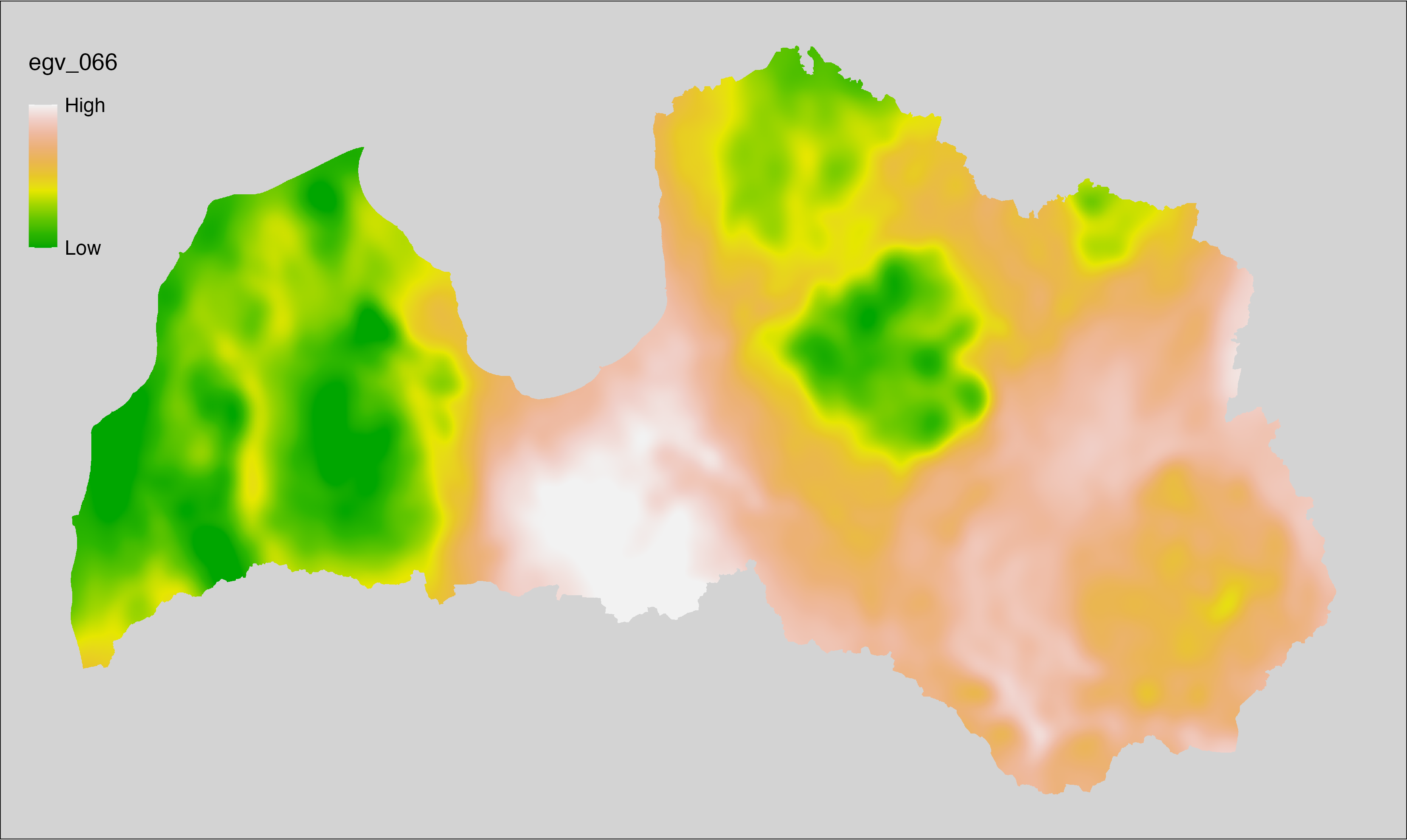
6.67 Climate_CHELSAv2.1-vpd-mean_cell
filename: Climate_CHELSAv2.1-vpd-mean_cell.tif
layername: egv_067
English name: Mean of monthly mean vapor pressure deficit (Pa) (CHELSA v2.1) within the analysis cell (1 ha)
Latvian name: Vidējais ik mēneša vidējais iztvaikošanas spiediena deficīts (Pa) (CHELSA v2.1) analīzes šūnā (1 ha)
Procedure: Directly follows CHELSA v2.1. EGV is prepared using
the workflow egvtools::downscale2egv() with inverse distance weighted (power =
2) gap filling and soft smoothing (power = 0.5) over 5 km radius around each cell.
Finally, the layer is standardised by subtracting the arithmetic mean and
dividing by the root mean squared error.
Code
# libs ----
if(!require(egvtools)) {remotes::install_github("aavotins/egvtools"); require(egvtools)}
# job ----
localname="Climate_CHELSAv2.1-vpd-mean_cell.tif"
layername="egv_067"
reading="./Geodata/2024/CHELSA/Climate_CHELSAv2.1-vpd-mean_cell.tif"
df <- downscale2egv(
template_path = "./Templates/TemplateRasters/LV100m_10km.tif",
grid_path = "./Templates/TemplateGrids/tikls1km_sauzeme.parquet",
rawfile_path = reading,
out_path = "./RasterGrids_100m/2024/RAW/",
file_name = localname,
layer_name = layername,
fill_gaps = TRUE,
smooth = TRUE,
smooth_radius_km = 5,
plot_result = TRUE)
print(df)
# standardisation ----
if(!require(terra)) {install.packages("terra"); require(terra)}
if(!require(tidyverse)) {install.packages("tidyverse"); require(tidyverse)}
nosaukums="Climate_CHELSAv2.1-vpd-mean_cell.tif"
ielasisanas_cels=paste0("./RasterGrids_100m/2024/RAW/",nosaukums)
saglabasanas_cels=paste0("./RasterGrids_100m/2024/Scaled/",nosaukums)
slanis=rast(ielasisanas_cels)
videjais=global(slanis,fun="mean",na.rm=TRUE)
centrets=slanis-videjais[,1]
standartnovirze=terra::global(centrets,fun="rms",na.rm=TRUE)
merogots=centrets/standartnovirze[,1]
writeRaster(merogots,
filename=saglabasanas_cels,
overwrite=TRUE)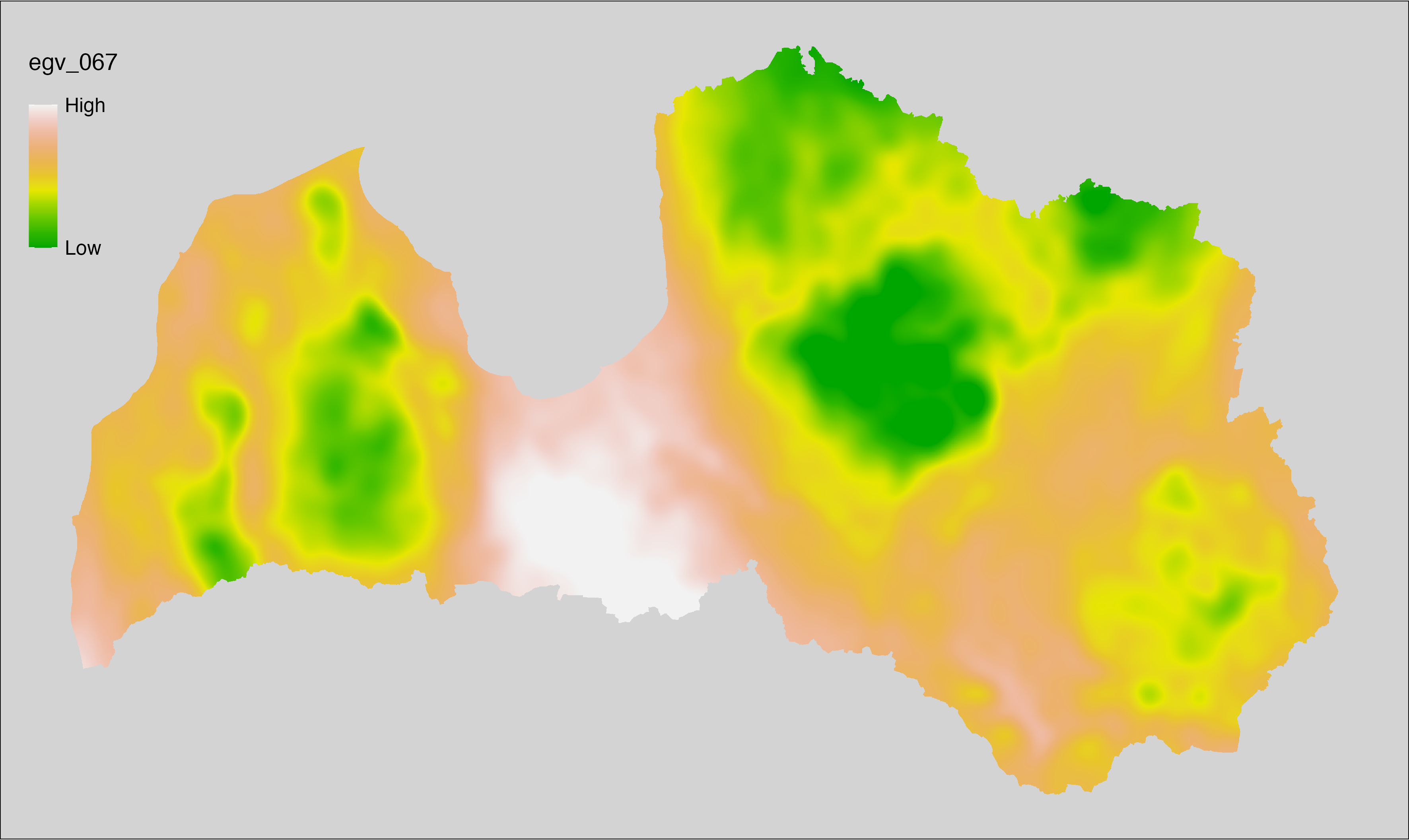
6.68 Climate_CHELSAv2.1-vpd-min_cell
filename: Climate_CHELSAv2.1-vpd-min_cell.tif
layername: egv_068
English name: Mean of monthly minimum vapor pressure deficit (Pa) (CHELSA v2.1) within the analysis cell (1 ha)
Latvian name: Vidējais ik mēneša minimālais iztvaikošanas spiediena deficīts (Pa) (CHELSA v2.1) analīzes šūnā (1 ha)
Procedure: Directly follows CHELSA v2.1. EGV is prepared using
the workflow egvtools::downscale2egv() with inverse distance weighted (power =
2) gap filling and soft smoothing (power = 0.5) over 5 km radius around each cell.
Finally, the layer is standardised by subtracting the arithmetic mean and
dividing by the root mean squared error.
Code
# libs ----
if(!require(egvtools)) {remotes::install_github("aavotins/egvtools"); require(egvtools)}
# job ----
localname="Climate_CHELSAv2.1-vpd-min_cell.tif"
layername="egv_068"
reading="./Geodata/2024/CHELSA/Climate_CHELSAv2.1-vpd-min_cell.tif"
df <- downscale2egv(
template_path = "./Templates/TemplateRasters/LV100m_10km.tif",
grid_path = "./Templates/TemplateGrids/tikls1km_sauzeme.parquet",
rawfile_path = reading,
out_path = "./RasterGrids_100m/2024/RAW/",
file_name = localname,
layer_name = layername,
fill_gaps = TRUE,
smooth = TRUE,
smooth_radius_km = 5,
plot_result = TRUE)
print(df)
# standardisation ----
if(!require(terra)) {install.packages("terra"); require(terra)}
if(!require(tidyverse)) {install.packages("tidyverse"); require(tidyverse)}
nosaukums="Climate_CHELSAv2.1-vpd-min_cell.tif"
ielasisanas_cels=paste0("./RasterGrids_100m/2024/RAW/",nosaukums)
saglabasanas_cels=paste0("./RasterGrids_100m/2024/Scaled/",nosaukums)
slanis=rast(ielasisanas_cels)
videjais=global(slanis,fun="mean",na.rm=TRUE)
centrets=slanis-videjais[,1]
standartnovirze=terra::global(centrets,fun="rms",na.rm=TRUE)
merogots=centrets/standartnovirze[,1]
writeRaster(merogots,
filename=saglabasanas_cels,
overwrite=TRUE)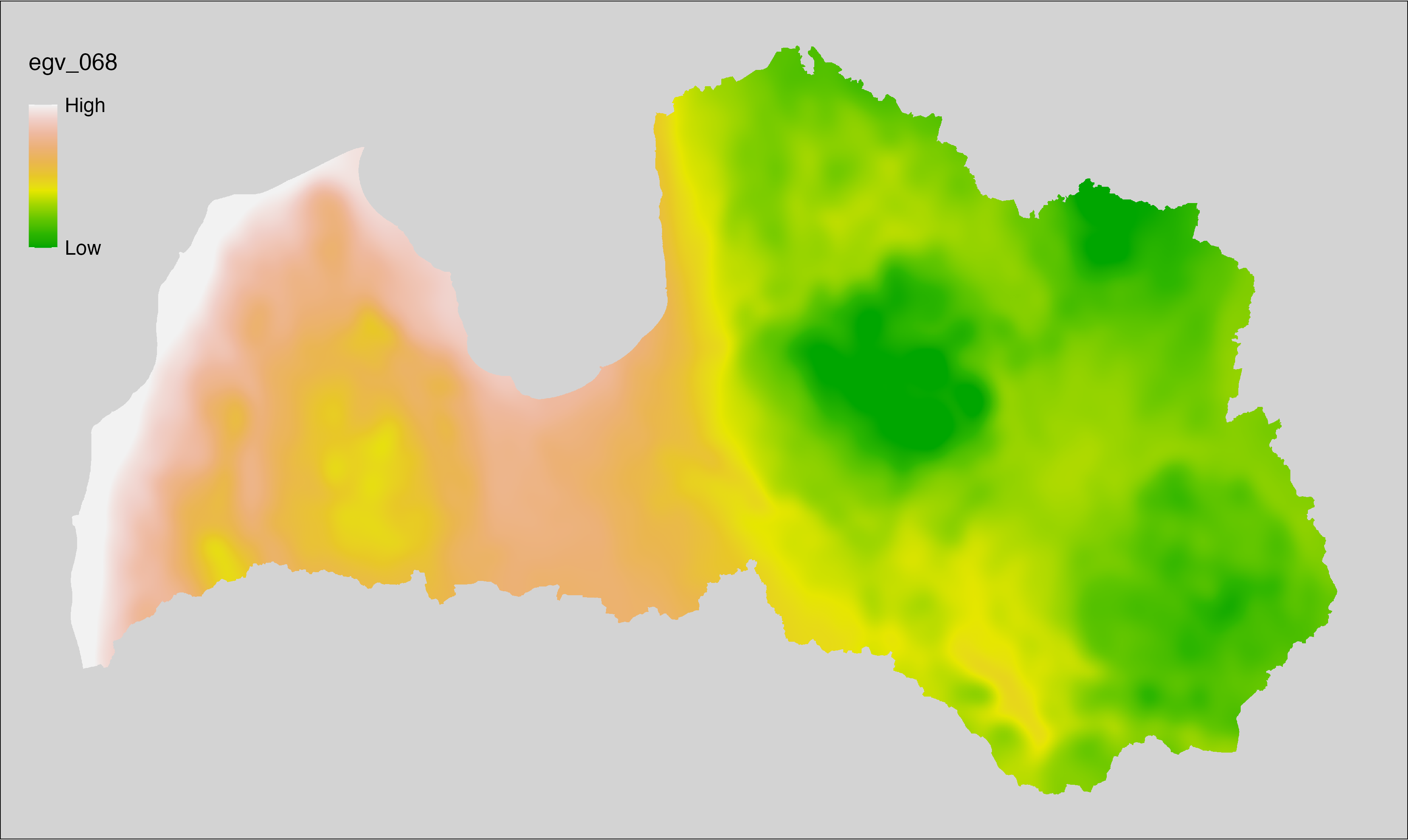
6.69 Climate_CHELSAv2.1-vpd-range_cell
filename: Climate_CHELSAv2.1-vpd-range_cell.tif
layername: egv_069
English name: Annual range of monthly mean vapor pressure deficit (Pa) (CHELSA v2.1) within the analysis cell (1 ha)
Latvian name: Gada iztvaikošanas spiediena deficīta ik mēneša vidējo amplitūda (Pa) (CHELSA v2.1) analīzes šūnā (1 ha)
Procedure: Directly follows CHELSA v2.1. EGV is prepared using
the workflow egvtools::downscale2egv() with inverse distance weighted (power =
2) gap filling and soft smoothing (power = 0.5) over 5 km radius around each cell.
Finally, the layer is standardised by subtracting the arithmetic mean and
dividing by the root mean squared error.
Code
# libs ----
if(!require(egvtools)) {remotes::install_github("aavotins/egvtools"); require(egvtools)}
# job ----
localname="Climate_CHELSAv2.1-vpd-range_cell.tif"
layername="egv_069"
reading="./Geodata/2024/CHELSA/Climate_CHELSAv2.1-vpd-range_cell.tif"
df <- downscale2egv(
template_path = "./Templates/TemplateRasters/LV100m_10km.tif",
grid_path = "./Templates/TemplateGrids/tikls1km_sauzeme.parquet",
rawfile_path = reading,
out_path = "./RasterGrids_100m/2024/RAW/",
file_name = localname,
layer_name = layername,
fill_gaps = TRUE,
smooth = TRUE,
smooth_radius_km = 5,
plot_result = TRUE)
print(df)
# standardisation ----
if(!require(terra)) {install.packages("terra"); require(terra)}
if(!require(tidyverse)) {install.packages("tidyverse"); require(tidyverse)}
nosaukums="Climate_CHELSAv2.1-vpd-range_cell.tif"
ielasisanas_cels=paste0("./RasterGrids_100m/2024/RAW/",nosaukums)
saglabasanas_cels=paste0("./RasterGrids_100m/2024/Scaled/",nosaukums)
slanis=rast(ielasisanas_cels)
videjais=global(slanis,fun="mean",na.rm=TRUE)
centrets=slanis-videjais[,1]
standartnovirze=terra::global(centrets,fun="rms",na.rm=TRUE)
merogots=centrets/standartnovirze[,1]
writeRaster(merogots,
filename=saglabasanas_cels,
overwrite=TRUE)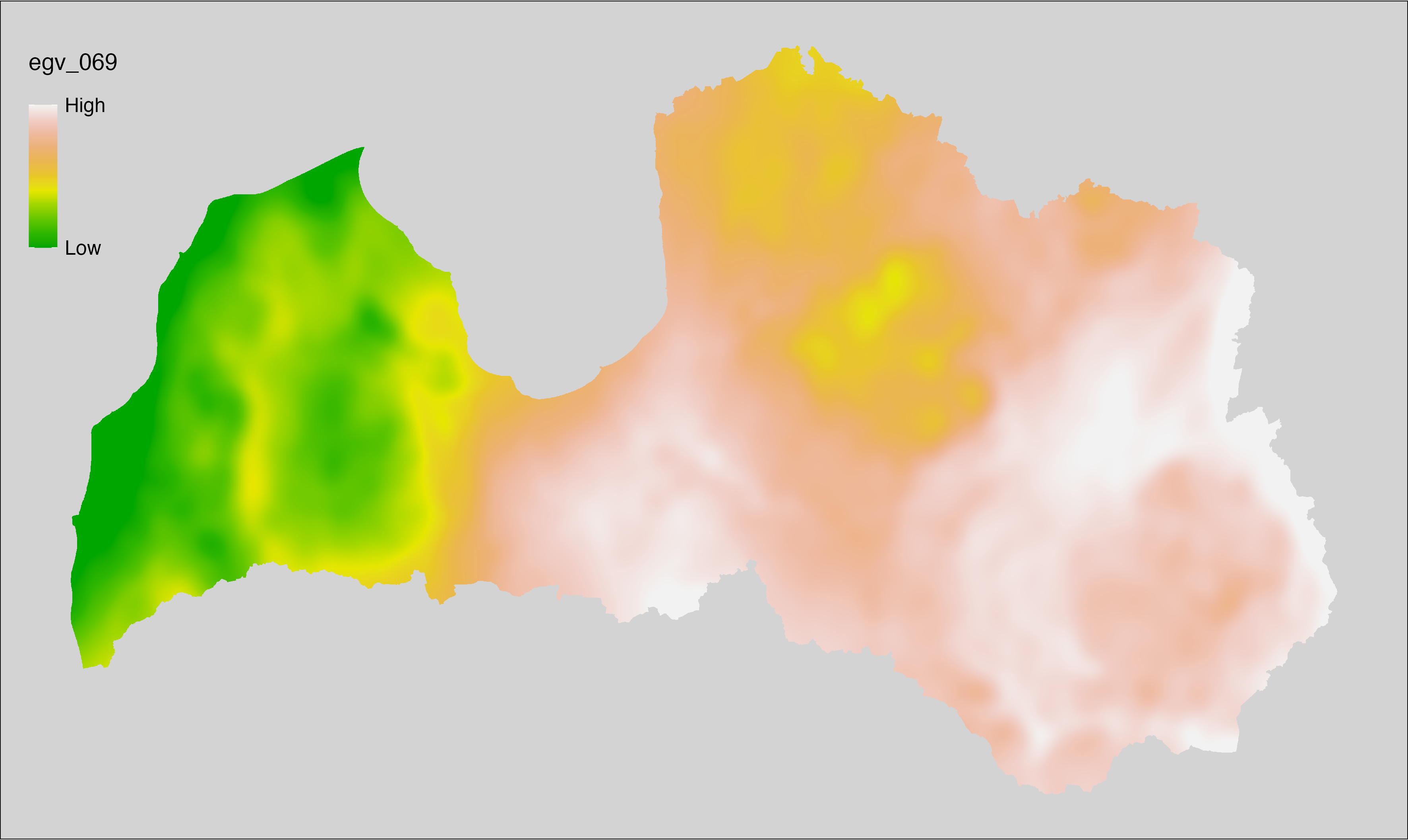
6.70 HydroClim_01-max_cell
filename: HydroClim_01-max_cell.tif
layername: egv_070
English name: Maximum per subcatchment upstream mean annual air temperature (°C) (HydroClim) within the analysis cell (1 ha)
Latvian name: Sateces apakšbaseina maksimālā vidējā gaisa temperatūra augštecē (°C) (HydroClim) analīzes šūnā (1 ha)
Procedure: Information from the HydroClim
data - including both basin and raster layers - is used. First, basin CRS is transformed to EPSG:3059. Then,
zonal statistics (per basin) using a layer specific summary function (max) are
calculated (exactextractr::exact_extract()), and the the results are rasterised with the workflow
egvtools::polygon2input(). Once rasterised to input data, EGV is created using the workflow
egvtools::input2egv(). To prevent from gaps at the edges, inverse distance
weighted (power = 2) gap filling is implemented. To save disk space,
the intermediate input layer is unlinked. Finally, the layer is standardised by
subtracting the arithmetic mean and dividing by the root mean squared error.
Code
# libs ----
if(!require(egvtools)) {remotes::install_github("aavotins/egvtools"); require(egvtools)}
if(!require(terra)) {install.packages("terra"); require(terra)}
if(!require(tidyverse)) {install.packages("tidyverse"); require(tidyverse)}
if(!require(sf)) {install.packages("sf"); require(sf)}
if(!require(sfarrow)) {install.packages("sfarrow"); require(sfarrow)}
if(!require(exactextractr)) {install.packages("exactextractr"); require(exactextractr)}
# basins ----
level12=st_read("./Geodata/2024/HydroClim/hybas_lake_eu_lev01-12_v1c/hybas_lake_eu_lev12_v1c.shp")
grid_1km=sfarrow::st_read_parquet("./Templates/TemplateGrids/tikls1km_sauzeme.parquet")
grid_1km=st_transform(grid_1km,crs=3059)
level12=st_transform(level12,crs=3059)
level12=level12[grid_1km,,]
level12=st_make_valid(level12)
# job ----
localname="HydroClim_01-max_cell.tif"
layername="egv_070"
summary_function="max"
slanis=rast(paste0("./Geodata/2024/HydroClim/",localname))
level12$Hydro_values=exact_extract(slanis,level12,fun=summary_function)
polygon2input(vector_data = level12,
template_path = "./Templates/TemplateRasters/LV10m_10km.tif",
out_path = "./RasterGrids_10m/2024/",
file_name = localname,
value_field = "Hydro_values",
fun="first",
value_type = "continuous",
prepare=FALSE,
project_mode = "auto",
check_na = FALSE,
plot_result=FALSE,
plot_gaps = FALSE,
overwrite=TRUE)
egvrez=input2egv(input=paste0("./RasterGrids_10m/2024/",localname),
egv_template= "./Templates/TemplateRasters/LV100m_10km.tif",
summary_function = "average",
missing_job = "FillOutput",
input_template = "./Templates/TemplateRasters/LV10m_10km.tif",
outlocation = "./RasterGrids_100m/2024/RAW/",
outfilename = localname,
layername = layername,
idw_weight = 2,
plot_gaps = FALSE,plot_final = FALSE)
egvrez
unlink(paste0("./RasterGrids_10m/2024/",localname))
# standardisation ----
if(!require(terra)) {install.packages("terra"); require(terra)}
if(!require(tidyverse)) {install.packages("tidyverse"); require(tidyverse)}
nosaukums="HydroClim_01-max_cell.tif"
ielasisanas_cels=paste0("./RasterGrids_100m/2024/RAW/",nosaukums)
saglabasanas_cels=paste0("./RasterGrids_100m/2024/Scaled/",nosaukums)
slanis=rast(ielasisanas_cels)
videjais=global(slanis,fun="mean",na.rm=TRUE)
centrets=slanis-videjais[,1]
standartnovirze=terra::global(centrets,fun="rms",na.rm=TRUE)
merogots=centrets/standartnovirze[,1]
writeRaster(merogots,
filename=saglabasanas_cels,
overwrite=TRUE)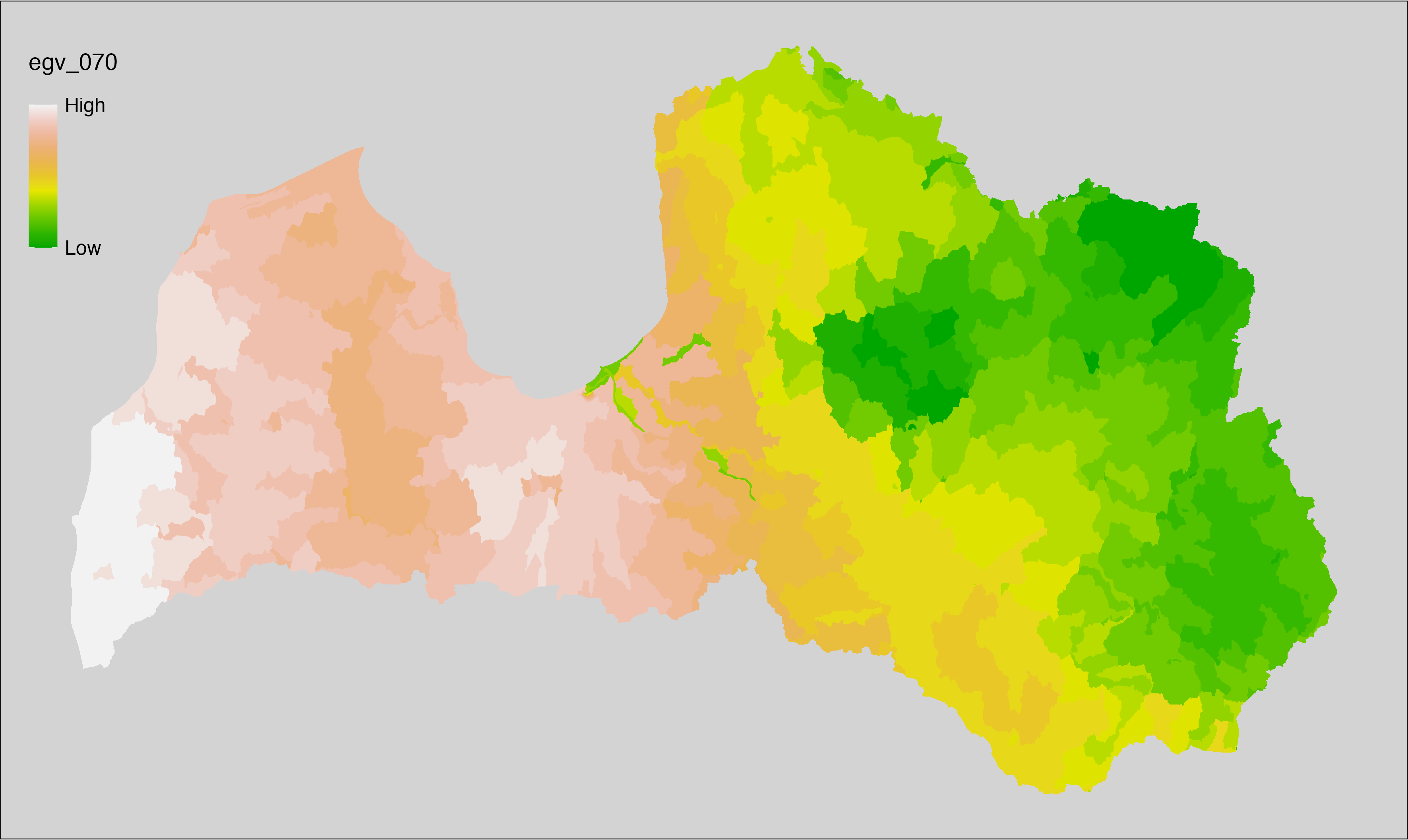
6.71 HydroClim_02-max_cell
filename: HydroClim_02-max_cell.tif
layername: egv_071
English name: Maximum per subcatchment upstream mean diurnal air temperature range (°C) (HydroClim) within the analysis cell (1 ha)
Latvian name: Sateces apakšbaseina maksimālā diennakts gaisa temperatūras amplitūda augštecē (°C) (HydroClim) analīzes šūnā (1 ha)
Procedure: Information from the HydroClim
data - including both basin and raster layers - is used. First, basin CRS is transformed to EPSG:3059. Then,
zonal statistics (per basin) using a layer specific summary function (max) are
calculated (exactextractr::exact_extract()), and the the results are rasterised with the workflow
egvtools::polygon2input(). Once rasterised to input data, EGV is created using the workflow
egvtools::input2egv(). To prevent from gaps at the edges, inverse distance
weighted (power = 2) gap filling is implemented. To save disk space,
the intermediate input layer is unlinked. Finally, the layer is standardised by
subtracting the arithmetic mean and dividing by the root mean squared error.
Code
# libs ----
if(!require(egvtools)) {remotes::install_github("aavotins/egvtools"); require(egvtools)}
if(!require(terra)) {install.packages("terra"); require(terra)}
if(!require(tidyverse)) {install.packages("tidyverse"); require(tidyverse)}
if(!require(sf)) {install.packages("sf"); require(sf)}
if(!require(sfarrow)) {install.packages("sfarrow"); require(sfarrow)}
if(!require(exactextractr)) {install.packages("exactextractr"); require(exactextractr)}
# basins ----
level12=st_read("./Geodata/2024/HydroClim/hybas_lake_eu_lev01-12_v1c/hybas_lake_eu_lev12_v1c.shp")
grid_1km=sfarrow::st_read_parquet("./Templates/TemplateGrids/tikls1km_sauzeme.parquet")
grid_1km=st_transform(grid_1km,crs=3059)
level12=st_transform(level12,crs=3059)
level12=level12[grid_1km,,]
level12=st_make_valid(level12)
# job ----
localname="HydroClim_02-max_cell.tif"
layername="egv_071"
summary_function="max"
slanis=rast(paste0("./Geodata/2024/HydroClim/",localname))
level12$Hydro_values=exact_extract(slanis,level12,fun=summary_function)
polygon2input(vector_data = level12,
template_path = "./Templates/TemplateRasters/LV10m_10km.tif",
out_path = "./RasterGrids_10m/2024/",
file_name = localname,
value_field = "Hydro_values",
fun="first",
value_type = "continuous",
prepare=FALSE,
project_mode = "auto",
check_na = FALSE,
plot_result=FALSE,
plot_gaps = FALSE,
overwrite=TRUE)
egvrez=input2egv(input=paste0("./RasterGrids_10m/2024/",localname),
egv_template= "./Templates/TemplateRasters/LV100m_10km.tif",
summary_function = "average",
missing_job = "FillOutput",
input_template = "./Templates/TemplateRasters/LV10m_10km.tif",
outlocation = "./RasterGrids_100m/2024/RAW/",
outfilename = localname,
layername = layername,
idw_weight = 2,
plot_gaps = FALSE,plot_final = FALSE)
egvrez
unlink(paste0("./RasterGrids_10m/2024/",localname))
# standardisation ----
if(!require(terra)) {install.packages("terra"); require(terra)}
if(!require(tidyverse)) {install.packages("tidyverse"); require(tidyverse)}
nosaukums="HydroClim_02-max_cell.tif"
ielasisanas_cels=paste0("./RasterGrids_100m/2024/RAW/",nosaukums)
saglabasanas_cels=paste0("./RasterGrids_100m/2024/Scaled/",nosaukums)
slanis=rast(ielasisanas_cels)
videjais=global(slanis,fun="mean",na.rm=TRUE)
centrets=slanis-videjais[,1]
standartnovirze=terra::global(centrets,fun="rms",na.rm=TRUE)
merogots=centrets/standartnovirze[,1]
writeRaster(merogots,
filename=saglabasanas_cels,
overwrite=TRUE)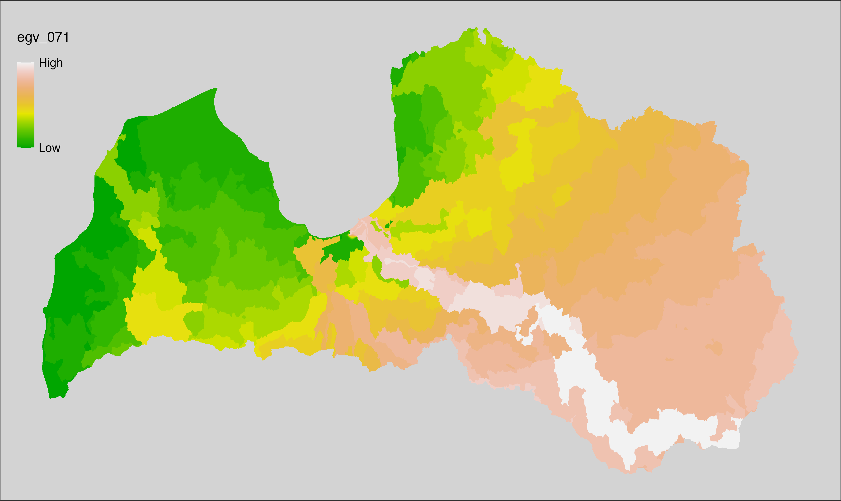
6.72 HydroClim_03-max_cell
filename: HydroClim_03-max_cell.tif
layername: egv_072
English name: Maximum per subcatchment upstream isothermality (ratio of diurnal variation to annual variation in temperatures) (°C) (HydroClim) within the analysis cell (1 ha)
Latvian name: Sateces apakšbaseina maksimālā izotermalitāte (diennakts un gada temperatūru variabilitātes attiecība) augštecē (°C) (HydroClim) analīzes šūnā (1 ha)
Procedure: Information from the HydroClim
data - including both basin and raster layers - is used. First, basin CRS is transformed to EPSG:3059. Then,
zonal statistics (per basin) using a layer specific summary function (max) are
calculated (exactextractr::exact_extract()), and the the results are rasterised with the workflow
egvtools::polygon2input(). Once rasterised to input data, EGV is created using the workflow
egvtools::input2egv(). To prevent from gaps at the edges, inverse distance
weighted (power = 2) gap filling is implemented. To save disk space,
the intermediate input layer is unlinked. Finally, the layer is standardised by
subtracting the arithmetic mean and dividing by the root mean squared error.
Code
# libs ----
if(!require(egvtools)) {remotes::install_github("aavotins/egvtools"); require(egvtools)}
if(!require(terra)) {install.packages("terra"); require(terra)}
if(!require(tidyverse)) {install.packages("tidyverse"); require(tidyverse)}
if(!require(sf)) {install.packages("sf"); require(sf)}
if(!require(sfarrow)) {install.packages("sfarrow"); require(sfarrow)}
if(!require(exactextractr)) {install.packages("exactextractr"); require(exactextractr)}
# basins ----
level12=st_read("./Geodata/2024/HydroClim/hybas_lake_eu_lev01-12_v1c/hybas_lake_eu_lev12_v1c.shp")
grid_1km=sfarrow::st_read_parquet("./Templates/TemplateGrids/tikls1km_sauzeme.parquet")
grid_1km=st_transform(grid_1km,crs=3059)
level12=st_transform(level12,crs=3059)
level12=level12[grid_1km,,]
level12=st_make_valid(level12)
# job ----
localname="HydroClim_03-max_cell.tif"
layername="egv_072"
summary_function="max"
slanis=rast(paste0("./Geodata/2024/HydroClim/",localname))
level12$Hydro_values=exact_extract(slanis,level12,fun=summary_function)
polygon2input(vector_data = level12,
template_path = "./Templates/TemplateRasters/LV10m_10km.tif",
out_path = "./RasterGrids_10m/2024/",
file_name = localname,
value_field = "Hydro_values",
fun="first",
value_type = "continuous",
prepare=FALSE,
project_mode = "auto",
check_na = FALSE,
plot_result=FALSE,
plot_gaps = FALSE,
overwrite=TRUE)
egvrez=input2egv(input=paste0("./RasterGrids_10m/2024/",localname),
egv_template= "./Templates/TemplateRasters/LV100m_10km.tif",
summary_function = "average",
missing_job = "FillOutput",
input_template = "./Templates/TemplateRasters/LV10m_10km.tif",
outlocation = "./RasterGrids_100m/2024/RAW/",
outfilename = localname,
layername = layername,
idw_weight = 2,
plot_gaps = FALSE,plot_final = FALSE)
egvrez
unlink(paste0("./RasterGrids_10m/2024/",localname))
# standardisation ----
if(!require(terra)) {install.packages("terra"); require(terra)}
if(!require(tidyverse)) {install.packages("tidyverse"); require(tidyverse)}
nosaukums="HydroClim_03-max_cell.tif"
ielasisanas_cels=paste0("./RasterGrids_100m/2024/RAW/",nosaukums)
saglabasanas_cels=paste0("./RasterGrids_100m/2024/Scaled/",nosaukums)
slanis=rast(ielasisanas_cels)
videjais=global(slanis,fun="mean",na.rm=TRUE)
centrets=slanis-videjais[,1]
standartnovirze=terra::global(centrets,fun="rms",na.rm=TRUE)
merogots=centrets/standartnovirze[,1]
writeRaster(merogots,
filename=saglabasanas_cels,
overwrite=TRUE)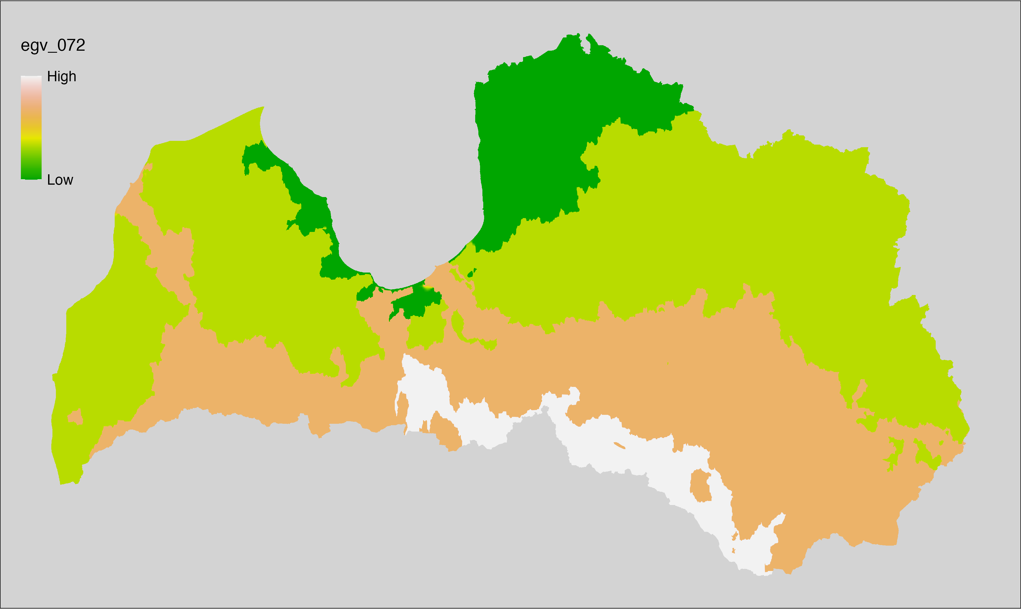
6.73 HydroClim_04-max_cell
filename: HydroClim_04-max_cell.tif
layername: egv_073
English name: Maximum per subcatchment upstream temperature seasonality (standard deviation of the monthly mean temperatures) (°C/100) (HydroClim) within the analysis cell (1 ha)
Latvian name: Sateces apakšbaseina maksimālā temperatūras sezonalitāte (mēneša vidējo temperatūru standartnovirze) augštecē (°C/100) (HydroClim) analīzes šūnā (1 ha)
Procedure: Information from the HydroClim
data - including both basin and raster layers - is used. First, basin CRS is transformed to EPSG:3059. Then,
zonal statistics (per basin) using a layer specific summary function (max) are
calculated (exactextractr::exact_extract()), and the the results are rasterised with the workflow
egvtools::polygon2input(). Once rasterised to input data, EGV is created using the workflow
egvtools::input2egv(). To prevent from gaps at the edges, inverse distance
weighted (power = 2) gap filling is implemented. To save disk space,
the intermediate input layer is unlinked. Finally, the layer is standardised by
subtracting the arithmetic mean and dividing by the root mean squared error.
Code
# libs ----
if(!require(egvtools)) {remotes::install_github("aavotins/egvtools"); require(egvtools)}
if(!require(terra)) {install.packages("terra"); require(terra)}
if(!require(tidyverse)) {install.packages("tidyverse"); require(tidyverse)}
if(!require(sf)) {install.packages("sf"); require(sf)}
if(!require(sfarrow)) {install.packages("sfarrow"); require(sfarrow)}
if(!require(exactextractr)) {install.packages("exactextractr"); require(exactextractr)}
# basins ----
level12=st_read("./Geodata/2024/HydroClim/hybas_lake_eu_lev01-12_v1c/hybas_lake_eu_lev12_v1c.shp")
grid_1km=sfarrow::st_read_parquet("./Templates/TemplateGrids/tikls1km_sauzeme.parquet")
grid_1km=st_transform(grid_1km,crs=3059)
level12=st_transform(level12,crs=3059)
level12=level12[grid_1km,,]
level12=st_make_valid(level12)
# job ----
localname="HydroClim_04-max_cell.tif"
layername="egv_073"
summary_function="max"
slanis=rast(paste0("./Geodata/2024/HydroClim/",localname))
level12$Hydro_values=exact_extract(slanis,level12,fun=summary_function)
polygon2input(vector_data = level12,
template_path = "./Templates/TemplateRasters/LV10m_10km.tif",
out_path = "./RasterGrids_10m/2024/",
file_name = localname,
value_field = "Hydro_values",
fun="first",
value_type = "continuous",
prepare=FALSE,
project_mode = "auto",
check_na = FALSE,
plot_result=FALSE,
plot_gaps = FALSE,
overwrite=TRUE)
egvrez=input2egv(input=paste0("./RasterGrids_10m/2024/",localname),
egv_template= "./Templates/TemplateRasters/LV100m_10km.tif",
summary_function = "average",
missing_job = "FillOutput",
input_template = "./Templates/TemplateRasters/LV10m_10km.tif",
outlocation = "./RasterGrids_100m/2024/RAW/",
outfilename = localname,
layername = layername,
idw_weight = 2,
plot_gaps = FALSE,plot_final = FALSE)
egvrez
unlink(paste0("./RasterGrids_10m/2024/",localname))
# standardisation ----
if(!require(terra)) {install.packages("terra"); require(terra)}
if(!require(tidyverse)) {install.packages("tidyverse"); require(tidyverse)}
nosaukums="HydroClim_04-max_cell.tif"
ielasisanas_cels=paste0("./RasterGrids_100m/2024/RAW/",nosaukums)
saglabasanas_cels=paste0("./RasterGrids_100m/2024/Scaled/",nosaukums)
slanis=rast(ielasisanas_cels)
videjais=global(slanis,fun="mean",na.rm=TRUE)
centrets=slanis-videjais[,1]
standartnovirze=terra::global(centrets,fun="rms",na.rm=TRUE)
merogots=centrets/standartnovirze[,1]
writeRaster(merogots,
filename=saglabasanas_cels,
overwrite=TRUE)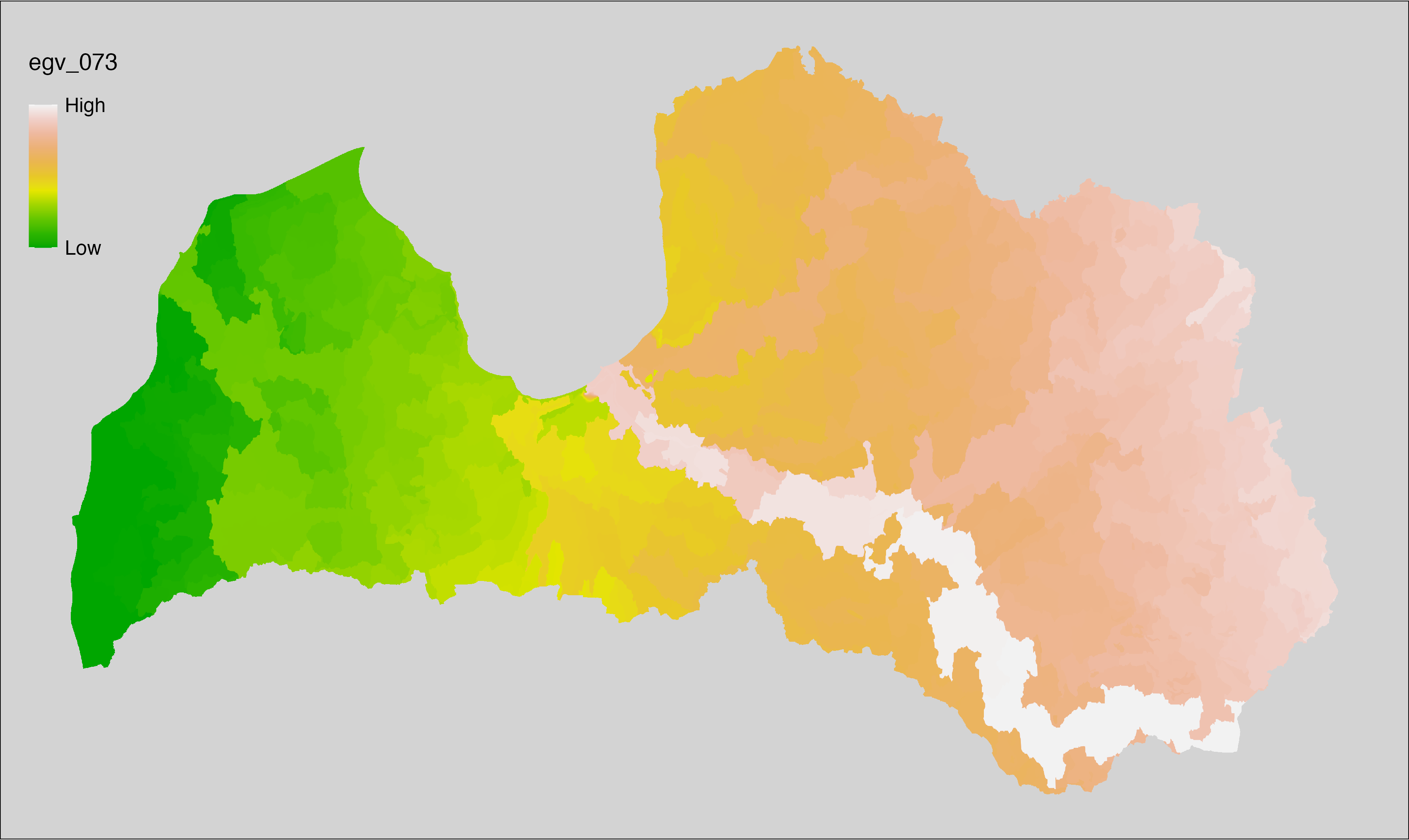
6.74 HydroClim_05-max_cell
filename: HydroClim_05-max_cell.tif
layername: egv_074
English name: Maximum per subcatchment upstream mean daily maximum air temperature (°C) of the warmest month (HydroClim) within the analysis cell (1 ha)
Latvian name: Sateces apakšbaseina maksimālā augšteces dienas augstākā gaisa temperatūra siltākajā mēnesī (°C) (HydroClim) analīzes šūnā (1 ha)
Procedure: Information from the HydroClim
data - including both basin and raster layers - is used. First, basin CRS is transformed to EPSG:3059. Then,
zonal statistics (per basin) using a layer specific summary function (max) are
calculated (exactextractr::exact_extract()), and the the results are rasterised with the workflow
egvtools::polygon2input(). Once rasterised to input data, EGV is created using the workflow
egvtools::input2egv(). To prevent from gaps at the edges, inverse distance
weighted (power = 2) gap filling is implemented. To save disk space,
the intermediate input layer is unlinked. Finally, the layer is standardised by
subtracting the arithmetic mean and dividing by the root mean squared error.
Code
# libs ----
if(!require(egvtools)) {remotes::install_github("aavotins/egvtools"); require(egvtools)}
if(!require(terra)) {install.packages("terra"); require(terra)}
if(!require(tidyverse)) {install.packages("tidyverse"); require(tidyverse)}
if(!require(sf)) {install.packages("sf"); require(sf)}
if(!require(sfarrow)) {install.packages("sfarrow"); require(sfarrow)}
if(!require(exactextractr)) {install.packages("exactextractr"); require(exactextractr)}
# basins ----
level12=st_read("./Geodata/2024/HydroClim/hybas_lake_eu_lev01-12_v1c/hybas_lake_eu_lev12_v1c.shp")
grid_1km=sfarrow::st_read_parquet("./Templates/TemplateGrids/tikls1km_sauzeme.parquet")
grid_1km=st_transform(grid_1km,crs=3059)
level12=st_transform(level12,crs=3059)
level12=level12[grid_1km,,]
level12=st_make_valid(level12)
# job ----
localname="HydroClim_05-max_cell.tif"
layername="egv_074"
summary_function="max"
slanis=rast(paste0("./Geodata/2024/HydroClim/",localname))
level12$Hydro_values=exact_extract(slanis,level12,fun=summary_function)
polygon2input(vector_data = level12,
template_path = "./Templates/TemplateRasters/LV10m_10km.tif",
out_path = "./RasterGrids_10m/2024/",
file_name = localname,
value_field = "Hydro_values",
fun="first",
value_type = "continuous",
prepare=FALSE,
project_mode = "auto",
check_na = FALSE,
plot_result=FALSE,
plot_gaps = FALSE,
overwrite=TRUE)
egvrez=input2egv(input=paste0("./RasterGrids_10m/2024/",localname),
egv_template= "./Templates/TemplateRasters/LV100m_10km.tif",
summary_function = "average",
missing_job = "FillOutput",
input_template = "./Templates/TemplateRasters/LV10m_10km.tif",
outlocation = "./RasterGrids_100m/2024/RAW/",
outfilename = localname,
layername = layername,
idw_weight = 2,
plot_gaps = FALSE,plot_final = FALSE)
egvrez
unlink(paste0("./RasterGrids_10m/2024/",localname))
# standardisation ----
if(!require(terra)) {install.packages("terra"); require(terra)}
if(!require(tidyverse)) {install.packages("tidyverse"); require(tidyverse)}
nosaukums="HydroClim_05-max_cell.tif"
ielasisanas_cels=paste0("./RasterGrids_100m/2024/RAW/",nosaukums)
saglabasanas_cels=paste0("./RasterGrids_100m/2024/Scaled/",nosaukums)
slanis=rast(ielasisanas_cels)
videjais=global(slanis,fun="mean",na.rm=TRUE)
centrets=slanis-videjais[,1]
standartnovirze=terra::global(centrets,fun="rms",na.rm=TRUE)
merogots=centrets/standartnovirze[,1]
writeRaster(merogots,
filename=saglabasanas_cels,
overwrite=TRUE)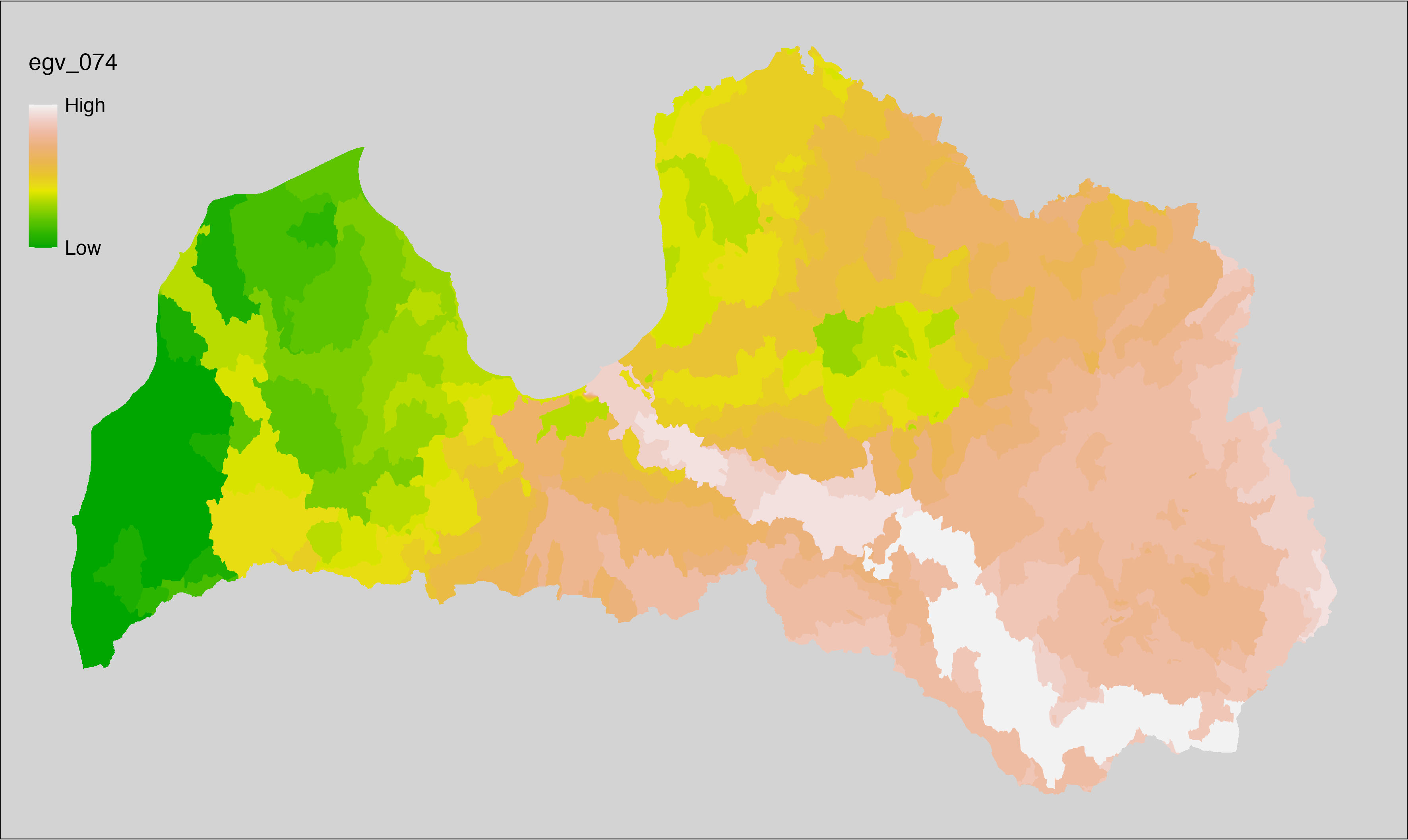
6.75 HydroClim_06-min_cell
filename: HydroClim_06-min_cell.tif
layername: egv_075
English name: Minimum per subcatchment upstream mean daily minimum air temperature (°C) of the coldest month (HydroClim) within the analysis cell (1 ha)
Latvian name: Sateces apakšbaseina minimālā augšteces dienas zemākā gaisa temperatūra vēsākajā mēnesī (°C) (HydroClim) analīzes šūnā (1 ha)
Procedure: Information from the HydroClim
data - including both basin and raster layers - is used. First, basin CRS is transformed to EPSG:3059. Then,
zonal statistics (per basin) using a layer specific summary function (min) are
calculated (exactextractr::exact_extract()), and the the results are rasterised with the workflow
egvtools::polygon2input(). Once rasterised to input data, EGV is created using the workflow
egvtools::input2egv(). To prevent from gaps at the edges, inverse distance
weighted (power = 2) gap filling is implemented. To save disk space,
the intermediate input layer is unlinked. Finally, the layer is standardised by
subtracting the arithmetic mean and dividing by the root mean squared error.
Code
# libs ----
if(!require(egvtools)) {remotes::install_github("aavotins/egvtools"); require(egvtools)}
if(!require(terra)) {install.packages("terra"); require(terra)}
if(!require(tidyverse)) {install.packages("tidyverse"); require(tidyverse)}
if(!require(sf)) {install.packages("sf"); require(sf)}
if(!require(sfarrow)) {install.packages("sfarrow"); require(sfarrow)}
if(!require(exactextractr)) {install.packages("exactextractr"); require(exactextractr)}
# basins ----
level12=st_read("./Geodata/2024/HydroClim/hybas_lake_eu_lev01-12_v1c/hybas_lake_eu_lev12_v1c.shp")
grid_1km=sfarrow::st_read_parquet("./Templates/TemplateGrids/tikls1km_sauzeme.parquet")
grid_1km=st_transform(grid_1km,crs=3059)
level12=st_transform(level12,crs=3059)
level12=level12[grid_1km,,]
level12=st_make_valid(level12)
# job ----
localname="HydroClim_06-min_cell.tif"
layername="egv_075"
summary_function="min"
slanis=rast(paste0("./Geodata/2024/HydroClim/",localname))
level12$Hydro_values=exact_extract(slanis,level12,fun=summary_function)
polygon2input(vector_data = level12,
template_path = "./Templates/TemplateRasters/LV10m_10km.tif",
out_path = "./RasterGrids_10m/2024/",
file_name = localname,
value_field = "Hydro_values",
fun="first",
value_type = "continuous",
prepare=FALSE,
project_mode = "auto",
check_na = FALSE,
plot_result=FALSE,
plot_gaps = FALSE,
overwrite=TRUE)
egvrez=input2egv(input=paste0("./RasterGrids_10m/2024/",localname),
egv_template= "./Templates/TemplateRasters/LV100m_10km.tif",
summary_function = "average",
missing_job = "FillOutput",
input_template = "./Templates/TemplateRasters/LV10m_10km.tif",
outlocation = "./RasterGrids_100m/2024/RAW/",
outfilename = localname,
layername = layername,
idw_weight = 2,
plot_gaps = FALSE,plot_final = FALSE)
egvrez
unlink(paste0("./RasterGrids_10m/2024/",localname))
# standardisation ----
if(!require(terra)) {install.packages("terra"); require(terra)}
if(!require(tidyverse)) {install.packages("tidyverse"); require(tidyverse)}
nosaukums="HydroClim_06-min_cell.tif"
ielasisanas_cels=paste0("./RasterGrids_100m/2024/RAW/",nosaukums)
saglabasanas_cels=paste0("./RasterGrids_100m/2024/Scaled/",nosaukums)
slanis=rast(ielasisanas_cels)
videjais=global(slanis,fun="mean",na.rm=TRUE)
centrets=slanis-videjais[,1]
standartnovirze=terra::global(centrets,fun="rms",na.rm=TRUE)
merogots=centrets/standartnovirze[,1]
writeRaster(merogots,
filename=saglabasanas_cels,
overwrite=TRUE)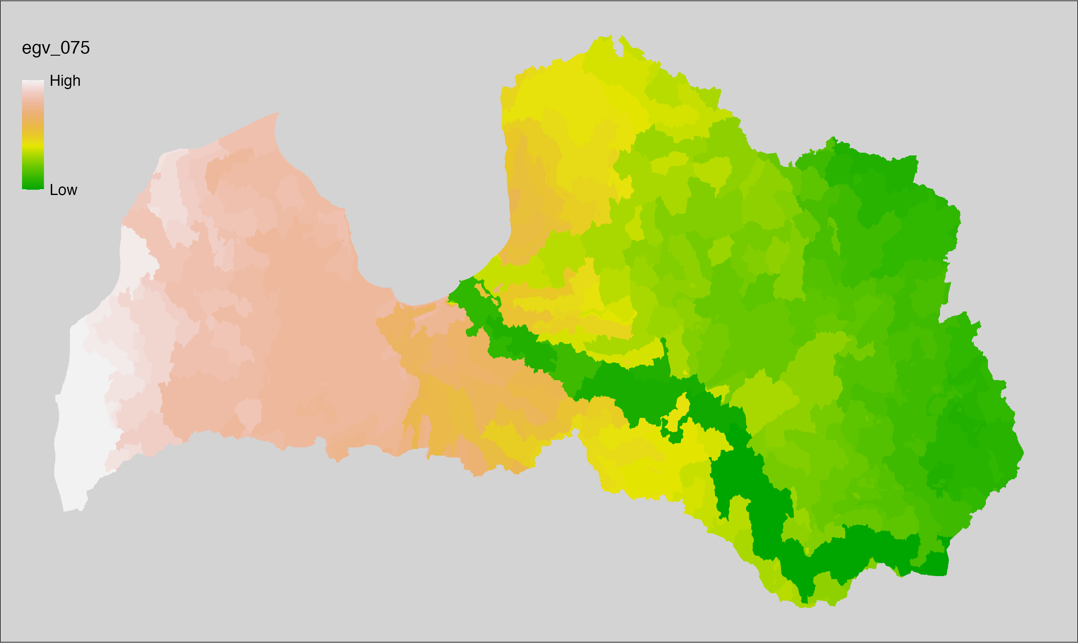
6.76 HydroClim_07-max_cell
filename: HydroClim_07-max_cell.tif
layername: egv_076
English name: Maximum per subcatchment upstream annual range of air temperature (°C) (HydroClim) within the analysis cell (1 ha)
Latvian name: Sateces apakšbaseina maksimālā augšteces gada gaisa temperatūru amplitūda (°C) (HydroClim) analīzes šūnā (1 ha)
Procedure: Information from the HydroClim
data - including both basin and raster layers - is used. First, basin CRS is transformed to EPSG:3059. Then,
zonal statistics (per basin) using a layer specific summary function (max) are
calculated (exactextractr::exact_extract()), and the the results are rasterised with the workflow
egvtools::polygon2input(). Once rasterised to input data, EGV is created using the workflow
egvtools::input2egv(). To prevent from gaps at the edges, inverse distance
weighted (power = 2) gap filling is implemented. To save disk space,
the intermediate input layer is unlinked. Finally, the layer is standardised by
subtracting the arithmetic mean and dividing by the root mean squared error.
Code
# libs ----
if(!require(egvtools)) {remotes::install_github("aavotins/egvtools"); require(egvtools)}
if(!require(terra)) {install.packages("terra"); require(terra)}
if(!require(tidyverse)) {install.packages("tidyverse"); require(tidyverse)}
if(!require(sf)) {install.packages("sf"); require(sf)}
if(!require(sfarrow)) {install.packages("sfarrow"); require(sfarrow)}
if(!require(exactextractr)) {install.packages("exactextractr"); require(exactextractr)}
# basins ----
level12=st_read("./Geodata/2024/HydroClim/hybas_lake_eu_lev01-12_v1c/hybas_lake_eu_lev12_v1c.shp")
grid_1km=sfarrow::st_read_parquet("./Templates/TemplateGrids/tikls1km_sauzeme.parquet")
grid_1km=st_transform(grid_1km,crs=3059)
level12=st_transform(level12,crs=3059)
level12=level12[grid_1km,,]
level12=st_make_valid(level12)
# job ----
localname="HydroClim_07-max_cell.tif"
layername="egv_076"
summary_function="max"
slanis=rast(paste0("./Geodata/2024/HydroClim/",localname))
level12$Hydro_values=exact_extract(slanis,level12,fun=summary_function)
polygon2input(vector_data = level12,
template_path = "./Templates/TemplateRasters/LV10m_10km.tif",
out_path = "./RasterGrids_10m/2024/",
file_name = localname,
value_field = "Hydro_values",
fun="first",
value_type = "continuous",
prepare=FALSE,
project_mode = "auto",
check_na = FALSE,
plot_result=FALSE,
plot_gaps = FALSE,
overwrite=TRUE)
egvrez=input2egv(input=paste0("./RasterGrids_10m/2024/",localname),
egv_template= "./Templates/TemplateRasters/LV100m_10km.tif",
summary_function = "average",
missing_job = "FillOutput",
input_template = "./Templates/TemplateRasters/LV10m_10km.tif",
outlocation = "./RasterGrids_100m/2024/RAW/",
outfilename = localname,
layername = layername,
idw_weight = 2,
plot_gaps = FALSE,plot_final = FALSE)
egvrez
unlink(paste0("./RasterGrids_10m/2024/",localname))
# standardisation ----
if(!require(terra)) {install.packages("terra"); require(terra)}
if(!require(tidyverse)) {install.packages("tidyverse"); require(tidyverse)}
nosaukums="HydroClim_07-max_cell.tif"
ielasisanas_cels=paste0("./RasterGrids_100m/2024/RAW/",nosaukums)
saglabasanas_cels=paste0("./RasterGrids_100m/2024/Scaled/",nosaukums)
slanis=rast(ielasisanas_cels)
videjais=global(slanis,fun="mean",na.rm=TRUE)
centrets=slanis-videjais[,1]
standartnovirze=terra::global(centrets,fun="rms",na.rm=TRUE)
merogots=centrets/standartnovirze[,1]
writeRaster(merogots,
filename=saglabasanas_cels,
overwrite=TRUE)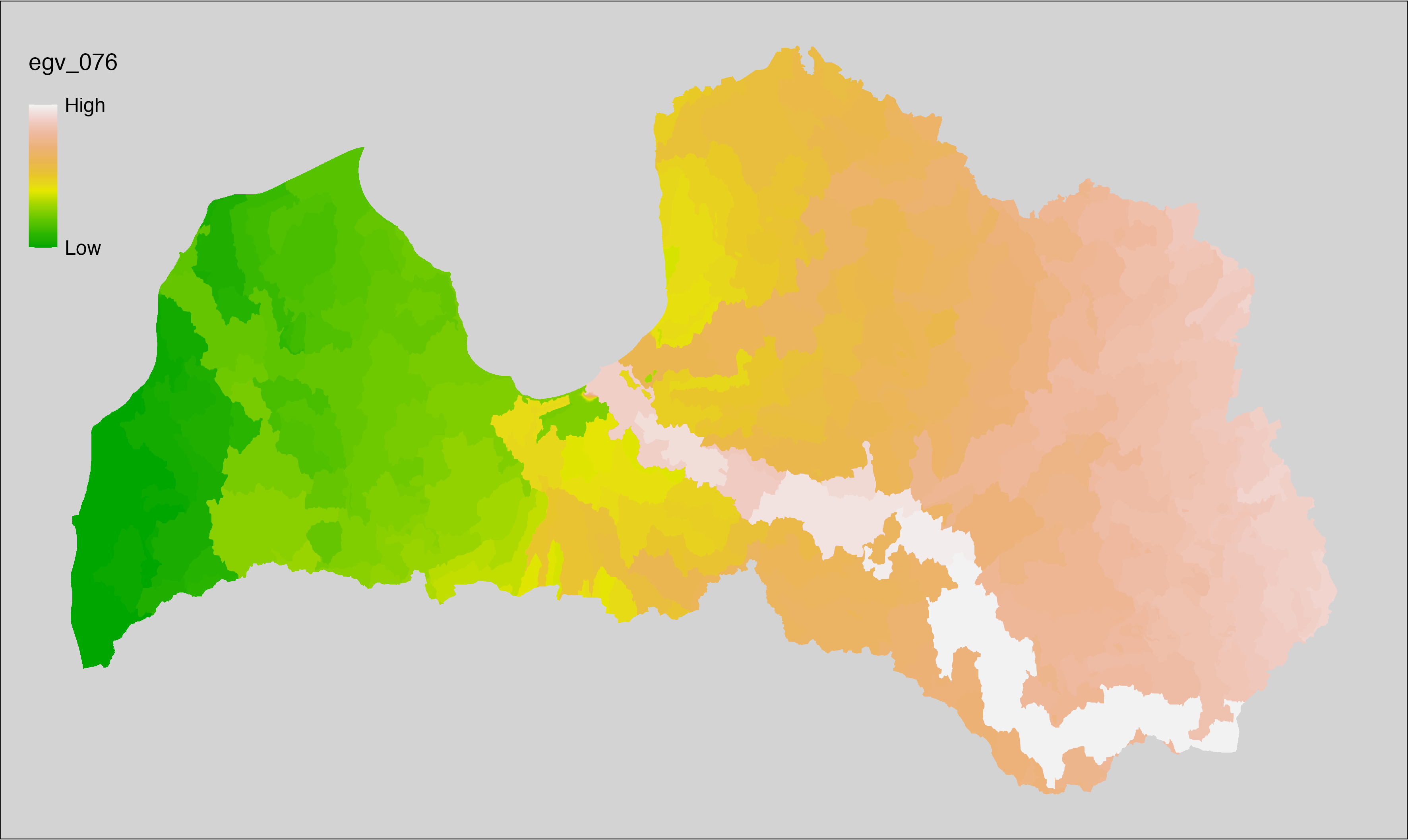
6.77 HydroClim_08-max_cell
filename: HydroClim_08-max_cell.tif
layername: egv_077
English name: Maximum per subcatchment upstream mean daily mean air temperatures (°C) of the wettest quarter (HydroClim) within the analysis cell (1 ha)
Latvian name: Sateces apakšbaseina maksimālā augšteces dienas vidējā gaisa temperatūra mitrākajā ceturksnī (°C) (HydroClim) analīzes šūnā (1 ha)
Procedure: Information from the HydroClim
data - including both basin and raster layers - is used. First, basin CRS is transformed to EPSG:3059. Then,
zonal statistics (per basin) using a layer specific summary function (max) are
calculated (exactextractr::exact_extract()), and the the results are rasterised with the workflow
egvtools::polygon2input(). Once rasterised to input data, EGV is created using the workflow
egvtools::input2egv(). To prevent from gaps at the edges, inverse distance
weighted (power = 2) gap filling is implemented. To save disk space,
the intermediate input layer is unlinked. Finally, the layer is standardised by
subtracting the arithmetic mean and dividing by the root mean squared error.
Code
# libs ----
if(!require(egvtools)) {remotes::install_github("aavotins/egvtools"); require(egvtools)}
if(!require(terra)) {install.packages("terra"); require(terra)}
if(!require(tidyverse)) {install.packages("tidyverse"); require(tidyverse)}
if(!require(sf)) {install.packages("sf"); require(sf)}
if(!require(sfarrow)) {install.packages("sfarrow"); require(sfarrow)}
if(!require(exactextractr)) {install.packages("exactextractr"); require(exactextractr)}
# basins ----
level12=st_read("./Geodata/2024/HydroClim/hybas_lake_eu_lev01-12_v1c/hybas_lake_eu_lev12_v1c.shp")
grid_1km=sfarrow::st_read_parquet("./Templates/TemplateGrids/tikls1km_sauzeme.parquet")
grid_1km=st_transform(grid_1km,crs=3059)
level12=st_transform(level12,crs=3059)
level12=level12[grid_1km,,]
level12=st_make_valid(level12)
# job ----
localname="HydroClim_08-max_cell.tif"
layername="egv_077"
summary_function="max"
slanis=rast(paste0("./Geodata/2024/HydroClim/",localname))
level12$Hydro_values=exact_extract(slanis,level12,fun=summary_function)
polygon2input(vector_data = level12,
template_path = "./Templates/TemplateRasters/LV10m_10km.tif",
out_path = "./RasterGrids_10m/2024/",
file_name = localname,
value_field = "Hydro_values",
fun="first",
value_type = "continuous",
prepare=FALSE,
project_mode = "auto",
check_na = FALSE,
plot_result=FALSE,
plot_gaps = FALSE,
overwrite=TRUE)
egvrez=input2egv(input=paste0("./RasterGrids_10m/2024/",localname),
egv_template= "./Templates/TemplateRasters/LV100m_10km.tif",
summary_function = "average",
missing_job = "FillOutput",
input_template = "./Templates/TemplateRasters/LV10m_10km.tif",
outlocation = "./RasterGrids_100m/2024/RAW/",
outfilename = localname,
layername = layername,
idw_weight = 2,
plot_gaps = FALSE,plot_final = FALSE)
egvrez
unlink(paste0("./RasterGrids_10m/2024/",localname))
# standardisation ----
if(!require(terra)) {install.packages("terra"); require(terra)}
if(!require(tidyverse)) {install.packages("tidyverse"); require(tidyverse)}
nosaukums="HydroClim_08-max_cell.tif"
ielasisanas_cels=paste0("./RasterGrids_100m/2024/RAW/",nosaukums)
saglabasanas_cels=paste0("./RasterGrids_100m/2024/Scaled/",nosaukums)
slanis=rast(ielasisanas_cels)
videjais=global(slanis,fun="mean",na.rm=TRUE)
centrets=slanis-videjais[,1]
standartnovirze=terra::global(centrets,fun="rms",na.rm=TRUE)
merogots=centrets/standartnovirze[,1]
writeRaster(merogots,
filename=saglabasanas_cels,
overwrite=TRUE)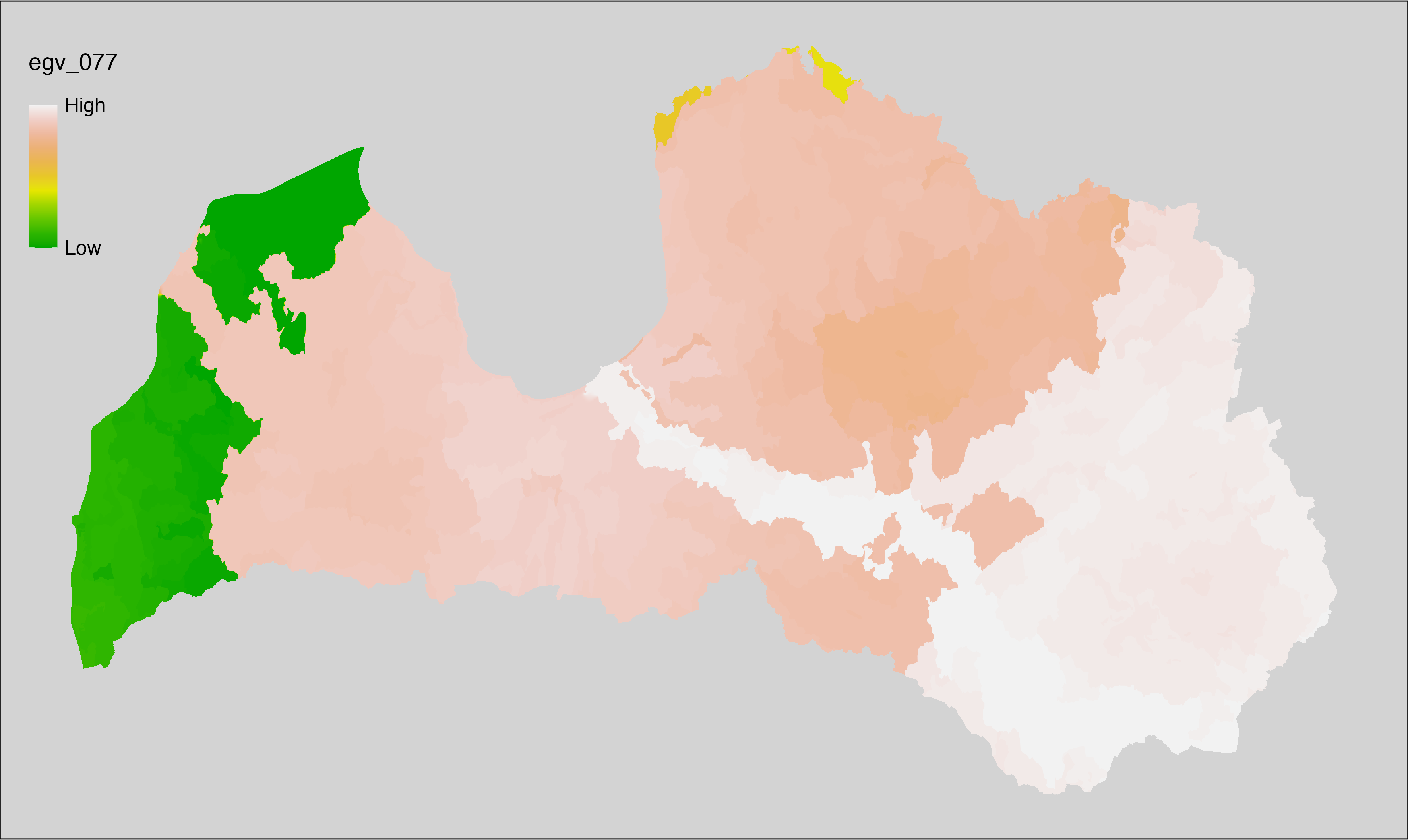
6.78 HydroClim_09-min_cell
filename: HydroClim_09-min_cell.tif
layername: egv_078
English name: Minimum per subcatchment upstream mean daily mean air temperatures (°C) of the driest quarter (HydroClim) within the analysis cell (1 ha)
Latvian name: Sateces apakšbaseina minimālā augšteces dienas vidējā gaisa temperatūra sausākajā ceturksnī (°C) (HydroClim) analīzes šūnā (1 ha)
Procedure: Information from the HydroClim
data - including both basin and raster layers - is used. First, basin CRS is transformed to EPSG:3059. Then,
zonal statistics (per basin) using a layer specific summary function (min) are
calculated (exactextractr::exact_extract()), and the the results are rasterised with the workflow
egvtools::polygon2input(). Once rasterised to input data, EGV is created using the workflow
egvtools::input2egv(). To prevent from gaps at the edges, inverse distance
weighted (power = 2) gap filling is implemented. To save disk space,
the intermediate input layer is unlinked. Finally, the layer is standardised by
subtracting the arithmetic mean and dividing by the root mean squared error.
Code
# libs ----
if(!require(egvtools)) {remotes::install_github("aavotins/egvtools"); require(egvtools)}
if(!require(terra)) {install.packages("terra"); require(terra)}
if(!require(tidyverse)) {install.packages("tidyverse"); require(tidyverse)}
if(!require(sf)) {install.packages("sf"); require(sf)}
if(!require(sfarrow)) {install.packages("sfarrow"); require(sfarrow)}
if(!require(exactextractr)) {install.packages("exactextractr"); require(exactextractr)}
# basins ----
level12=st_read("./Geodata/2024/HydroClim/hybas_lake_eu_lev01-12_v1c/hybas_lake_eu_lev12_v1c.shp")
grid_1km=sfarrow::st_read_parquet("./Templates/TemplateGrids/tikls1km_sauzeme.parquet")
grid_1km=st_transform(grid_1km,crs=3059)
level12=st_transform(level12,crs=3059)
level12=level12[grid_1km,,]
level12=st_make_valid(level12)
# job ----
localname="HydroClim_09-min_cell.tif"
layername="egv_078"
summary_function="min"
slanis=rast(paste0("./Geodata/2024/HydroClim/",localname))
level12$Hydro_values=exact_extract(slanis,level12,fun=summary_function)
polygon2input(vector_data = level12,
template_path = "./Templates/TemplateRasters/LV10m_10km.tif",
out_path = "./RasterGrids_10m/2024/",
file_name = localname,
value_field = "Hydro_values",
fun="first",
value_type = "continuous",
prepare=FALSE,
project_mode = "auto",
check_na = FALSE,
plot_result=FALSE,
plot_gaps = FALSE,
overwrite=TRUE)
egvrez=input2egv(input=paste0("./RasterGrids_10m/2024/",localname),
egv_template= "./Templates/TemplateRasters/LV100m_10km.tif",
summary_function = "average",
missing_job = "FillOutput",
input_template = "./Templates/TemplateRasters/LV10m_10km.tif",
outlocation = "./RasterGrids_100m/2024/RAW/",
outfilename = localname,
layername = layername,
idw_weight = 2,
plot_gaps = FALSE,plot_final = FALSE)
egvrez
unlink(paste0("./RasterGrids_10m/2024/",localname))
# standardisation ----
if(!require(terra)) {install.packages("terra"); require(terra)}
if(!require(tidyverse)) {install.packages("tidyverse"); require(tidyverse)}
nosaukums="HydroClim_09-min_cell.tif"
ielasisanas_cels=paste0("./RasterGrids_100m/2024/RAW/",nosaukums)
saglabasanas_cels=paste0("./RasterGrids_100m/2024/Scaled/",nosaukums)
slanis=rast(ielasisanas_cels)
videjais=global(slanis,fun="mean",na.rm=TRUE)
centrets=slanis-videjais[,1]
standartnovirze=terra::global(centrets,fun="rms",na.rm=TRUE)
merogots=centrets/standartnovirze[,1]
writeRaster(merogots,
filename=saglabasanas_cels,
overwrite=TRUE)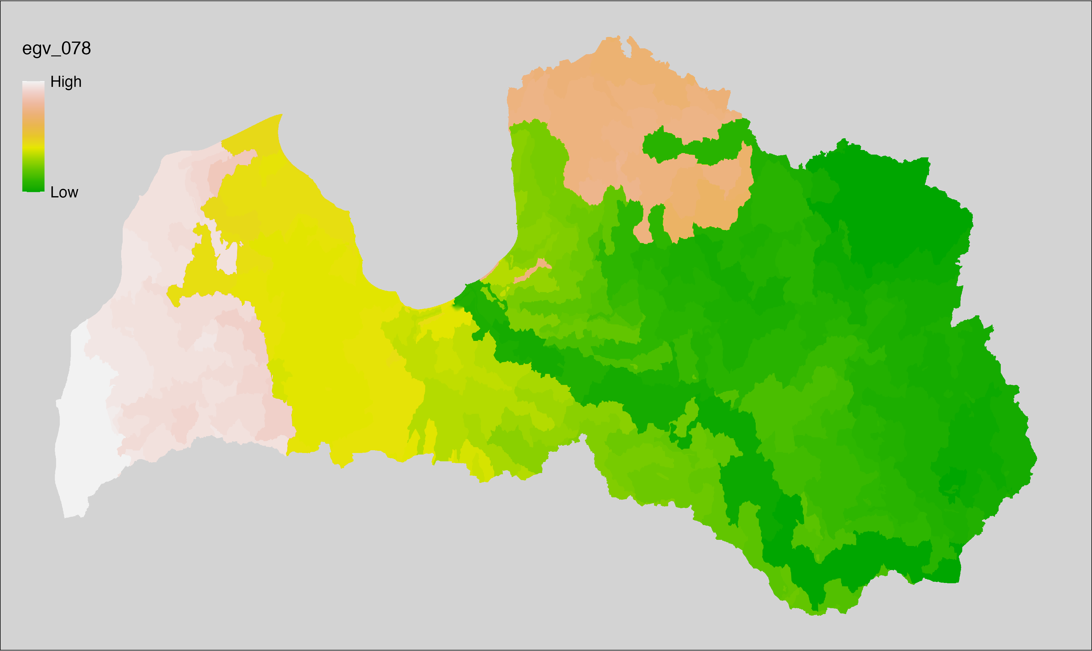
6.79 HydroClim_10-max_cell
filename: HydroClim_10-max_cell.tif
layername: egv_079
English name: Maximum per subcatchment upstream mean daily mean air temperatures (°C) of the warmest quarter (HydroClim) within the analysis cell (1 ha)
Latvian name: Sateces apakšbaseina maksimālā augšteces dienas vidējā gaisa temperatūra siltākajā ceturksnī (°C) (HydroClim) analīzes šūnā (1 ha)
Procedure: Information from the HydroClim
data - including both basin and raster layers - is used. First, basin CRS is transformed to EPSG:3059. Then,
zonal statistics (per basin) using a layer specific summary function (max) are
calculated (exactextractr::exact_extract()), and the the results are rasterised with the workflow
egvtools::polygon2input(). Once rasterised to input data, EGV is created using the workflow
egvtools::input2egv(). To prevent from gaps at the edges, inverse distance
weighted (power = 2) gap filling is implemented. To save disk space,
the intermediate input layer is unlinked. Finally, the layer is standardised by
subtracting the arithmetic mean and dividing by the root mean squared error.
Code
# libs ----
if(!require(egvtools)) {remotes::install_github("aavotins/egvtools"); require(egvtools)}
if(!require(terra)) {install.packages("terra"); require(terra)}
if(!require(tidyverse)) {install.packages("tidyverse"); require(tidyverse)}
if(!require(sf)) {install.packages("sf"); require(sf)}
if(!require(sfarrow)) {install.packages("sfarrow"); require(sfarrow)}
if(!require(exactextractr)) {install.packages("exactextractr"); require(exactextractr)}
# basins ----
level12=st_read("./Geodata/2024/HydroClim/hybas_lake_eu_lev01-12_v1c/hybas_lake_eu_lev12_v1c.shp")
grid_1km=sfarrow::st_read_parquet("./Templates/TemplateGrids/tikls1km_sauzeme.parquet")
grid_1km=st_transform(grid_1km,crs=3059)
level12=st_transform(level12,crs=3059)
level12=level12[grid_1km,,]
level12=st_make_valid(level12)
# job ----
localname="HydroClim_10-max_cell.tif"
layername="egv_079"
summary_function="max"
slanis=rast(paste0("./Geodata/2024/HydroClim/",localname))
level12$Hydro_values=exact_extract(slanis,level12,fun=summary_function)
polygon2input(vector_data = level12,
template_path = "./Templates/TemplateRasters/LV10m_10km.tif",
out_path = "./RasterGrids_10m/2024/",
file_name = localname,
value_field = "Hydro_values",
fun="first",
value_type = "continuous",
prepare=FALSE,
project_mode = "auto",
check_na = FALSE,
plot_result=FALSE,
plot_gaps = FALSE,
overwrite=TRUE)
egvrez=input2egv(input=paste0("./RasterGrids_10m/2024/",localname),
egv_template= "./Templates/TemplateRasters/LV100m_10km.tif",
summary_function = "average",
missing_job = "FillOutput",
input_template = "./Templates/TemplateRasters/LV10m_10km.tif",
outlocation = "./RasterGrids_100m/2024/RAW/",
outfilename = localname,
layername = layername,
idw_weight = 2,
plot_gaps = FALSE,plot_final = FALSE)
egvrez
unlink(paste0("./RasterGrids_10m/2024/",localname))
# standardisation ----
if(!require(terra)) {install.packages("terra"); require(terra)}
if(!require(tidyverse)) {install.packages("tidyverse"); require(tidyverse)}
nosaukums="HydroClim_10-max_cell.tif"
ielasisanas_cels=paste0("./RasterGrids_100m/2024/RAW/",nosaukums)
saglabasanas_cels=paste0("./RasterGrids_100m/2024/Scaled/",nosaukums)
slanis=rast(ielasisanas_cels)
videjais=global(slanis,fun="mean",na.rm=TRUE)
centrets=slanis-videjais[,1]
standartnovirze=terra::global(centrets,fun="rms",na.rm=TRUE)
merogots=centrets/standartnovirze[,1]
writeRaster(merogots,
filename=saglabasanas_cels,
overwrite=TRUE)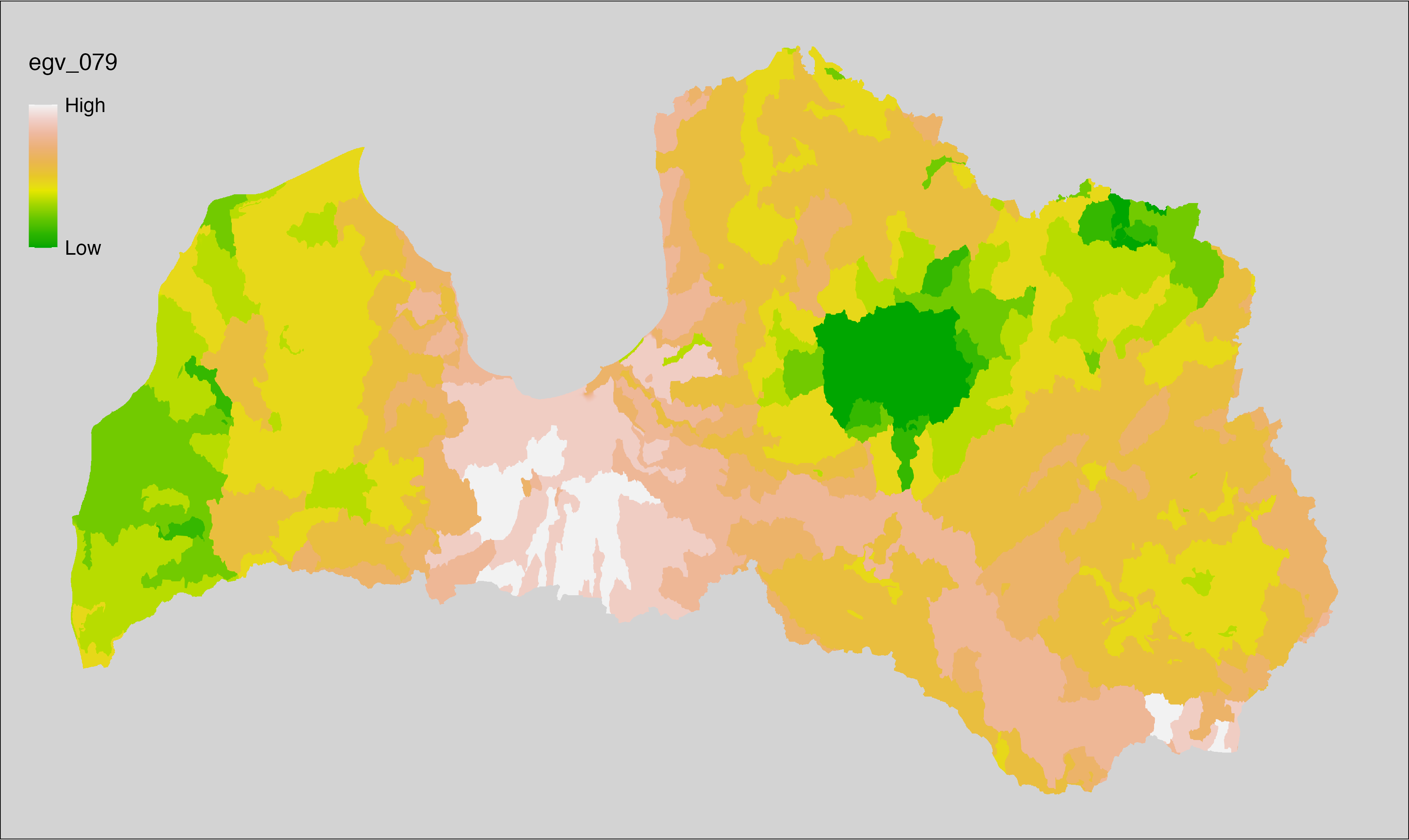
6.80 HydroClim_11-min_cell
filename: HydroClim_11-min_cell.tif
layername: egv_080
English name: Minimum per subcatchment upstream mean daily mean air temperatures (°C) of the coldest quarter (HydroClim) within the analysis cell (1 ha)
Latvian name: Sateces apakšbaseina minimālā augšteces dienas vidējā gaisa temperatūra vēsākajā ceturksnī (°C) (HydroClim) analīzes šūnā (1 ha)
Procedure: Information from the HydroClim
data - including both basin and raster layers - is used. First, basin CRS is transformed to EPSG:3059. Then,
zonal statistics (per basin) using a layer specific summary function (min) are
calculated (exactextractr::exact_extract()), and the the results are rasterised with the workflow
egvtools::polygon2input(). Once rasterised to input data, EGV is created using the workflow
egvtools::input2egv(). To prevent from gaps at the edges, inverse distance
weighted (power = 2) gap filling is implemented. To save disk space,
the intermediate input layer is unlinked. Finally, the layer is standardised by
subtracting the arithmetic mean and dividing by the root mean squared error.
Code
# libs ----
if(!require(egvtools)) {remotes::install_github("aavotins/egvtools"); require(egvtools)}
if(!require(terra)) {install.packages("terra"); require(terra)}
if(!require(tidyverse)) {install.packages("tidyverse"); require(tidyverse)}
if(!require(sf)) {install.packages("sf"); require(sf)}
if(!require(sfarrow)) {install.packages("sfarrow"); require(sfarrow)}
if(!require(exactextractr)) {install.packages("exactextractr"); require(exactextractr)}
# basins ----
level12=st_read("./Geodata/2024/HydroClim/hybas_lake_eu_lev01-12_v1c/hybas_lake_eu_lev12_v1c.shp")
grid_1km=sfarrow::st_read_parquet("./Templates/TemplateGrids/tikls1km_sauzeme.parquet")
grid_1km=st_transform(grid_1km,crs=3059)
level12=st_transform(level12,crs=3059)
level12=level12[grid_1km,,]
level12=st_make_valid(level12)
# job ----
localname="HydroClim_11-min_cell.tif"
layername="egv_080"
summary_function="min"
slanis=rast(paste0("./Geodata/2024/HydroClim/",localname))
level12$Hydro_values=exact_extract(slanis,level12,fun=summary_function)
polygon2input(vector_data = level12,
template_path = "./Templates/TemplateRasters/LV10m_10km.tif",
out_path = "./RasterGrids_10m/2024/",
file_name = localname,
value_field = "Hydro_values",
fun="first",
value_type = "continuous",
prepare=FALSE,
project_mode = "auto",
check_na = FALSE,
plot_result=FALSE,
plot_gaps = FALSE,
overwrite=TRUE)
egvrez=input2egv(input=paste0("./RasterGrids_10m/2024/",localname),
egv_template= "./Templates/TemplateRasters/LV100m_10km.tif",
summary_function = "average",
missing_job = "FillOutput",
input_template = "./Templates/TemplateRasters/LV10m_10km.tif",
outlocation = "./RasterGrids_100m/2024/RAW/",
outfilename = localname,
layername = layername,
idw_weight = 2,
plot_gaps = FALSE,plot_final = FALSE)
egvrez
unlink(paste0("./RasterGrids_10m/2024/",localname))
# standardisation ----
if(!require(terra)) {install.packages("terra"); require(terra)}
if(!require(tidyverse)) {install.packages("tidyverse"); require(tidyverse)}
nosaukums="HydroClim_11-min_cell.tif"
ielasisanas_cels=paste0("./RasterGrids_100m/2024/RAW/",nosaukums)
saglabasanas_cels=paste0("./RasterGrids_100m/2024/Scaled/",nosaukums)
slanis=rast(ielasisanas_cels)
videjais=global(slanis,fun="mean",na.rm=TRUE)
centrets=slanis-videjais[,1]
standartnovirze=terra::global(centrets,fun="rms",na.rm=TRUE)
merogots=centrets/standartnovirze[,1]
writeRaster(merogots,
filename=saglabasanas_cels,
overwrite=TRUE)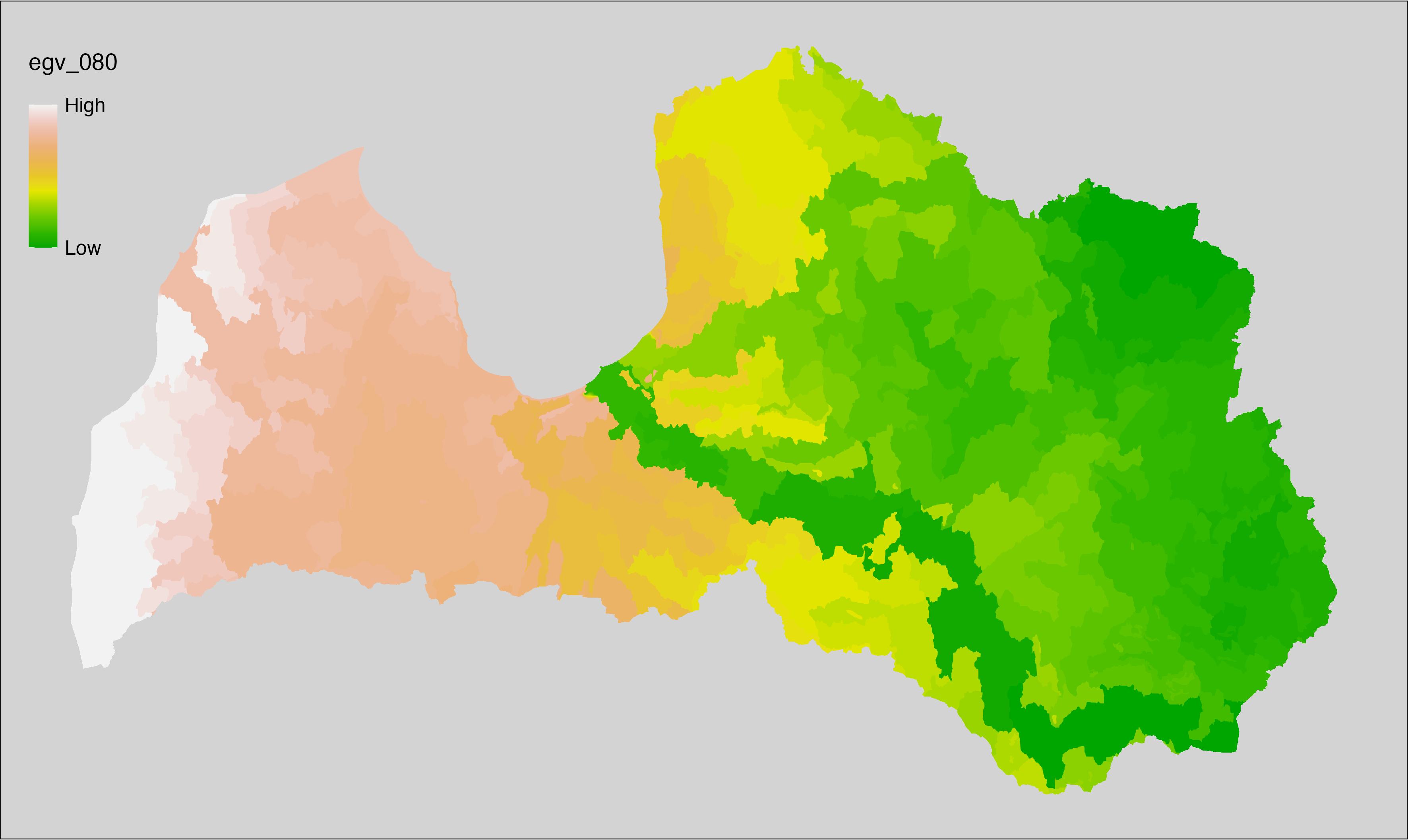
6.81 HydroClim_12-max_cell
filename: HydroClim_12-max_cell.tif
layername: egv_081
English name: Maximum per subcatchment upstream annual precipitation amount (kg m⁻² year⁻¹) (HydroClim) within the analysis cell (1 ha)
Latvian name: Sateces apakšbaseina maksimālais augšteces nokrišņu daudzums gadā (kg m⁻² year⁻¹) (HydroClim) analīzes šūnā (1 ha)
Procedure: Information from the HydroClim
data - including both basin and raster layers - is used. First, basin CRS is transformed to EPSG:3059. Then,
zonal statistics (per basin) using a layer specific summary function (max) are
calculated (exactextractr::exact_extract()), and the the results are rasterised with the workflow
egvtools::polygon2input(). Once rasterised to input data, EGV is created using the workflow
egvtools::input2egv(). To prevent from gaps at the edges, inverse distance
weighted (power = 2) gap filling is implemented. To save disk space,
the intermediate input layer is unlinked. Finally, the layer is standardised by
subtracting the arithmetic mean and dividing by the root mean squared error.
Code
# libs ----
if(!require(egvtools)) {remotes::install_github("aavotins/egvtools"); require(egvtools)}
if(!require(terra)) {install.packages("terra"); require(terra)}
if(!require(tidyverse)) {install.packages("tidyverse"); require(tidyverse)}
if(!require(sf)) {install.packages("sf"); require(sf)}
if(!require(sfarrow)) {install.packages("sfarrow"); require(sfarrow)}
if(!require(exactextractr)) {install.packages("exactextractr"); require(exactextractr)}
# basins ----
level12=st_read("./Geodata/2024/HydroClim/hybas_lake_eu_lev01-12_v1c/hybas_lake_eu_lev12_v1c.shp")
grid_1km=sfarrow::st_read_parquet("./Templates/TemplateGrids/tikls1km_sauzeme.parquet")
grid_1km=st_transform(grid_1km,crs=3059)
level12=st_transform(level12,crs=3059)
level12=level12[grid_1km,,]
level12=st_make_valid(level12)
# job ----
localname="HydroClim_12-max_cell.tif"
layername="egv_081"
summary_function="max"
slanis=rast(paste0("./Geodata/2024/HydroClim/",localname))
level12$Hydro_values=exact_extract(slanis,level12,fun=summary_function)
polygon2input(vector_data = level12,
template_path = "./Templates/TemplateRasters/LV10m_10km.tif",
out_path = "./RasterGrids_10m/2024/",
file_name = localname,
value_field = "Hydro_values",
fun="first",
value_type = "continuous",
prepare=FALSE,
project_mode = "auto",
check_na = FALSE,
plot_result=FALSE,
plot_gaps = FALSE,
overwrite=TRUE)
egvrez=input2egv(input=paste0("./RasterGrids_10m/2024/",localname),
egv_template= "./Templates/TemplateRasters/LV100m_10km.tif",
summary_function = "average",
missing_job = "FillOutput",
input_template = "./Templates/TemplateRasters/LV10m_10km.tif",
outlocation = "./RasterGrids_100m/2024/RAW/",
outfilename = localname,
layername = layername,
idw_weight = 2,
plot_gaps = FALSE,plot_final = FALSE)
egvrez
unlink(paste0("./RasterGrids_10m/2024/",localname))
# standardisation ----
if(!require(terra)) {install.packages("terra"); require(terra)}
if(!require(tidyverse)) {install.packages("tidyverse"); require(tidyverse)}
nosaukums="HydroClim_12-max_cell.tif"
ielasisanas_cels=paste0("./RasterGrids_100m/2024/RAW/",nosaukums)
saglabasanas_cels=paste0("./RasterGrids_100m/2024/Scaled/",nosaukums)
slanis=rast(ielasisanas_cels)
videjais=global(slanis,fun="mean",na.rm=TRUE)
centrets=slanis-videjais[,1]
standartnovirze=terra::global(centrets,fun="rms",na.rm=TRUE)
merogots=centrets/standartnovirze[,1]
writeRaster(merogots,
filename=saglabasanas_cels,
overwrite=TRUE)
6.82 HydroClim_13-max_cell
filename: HydroClim_13-max_cell.tif
layername: egv_082
English name: Maximum per subcatchment upstream precipitation amount (kg m⁻² year⁻¹) of the wettest month (HydroClim) within the analysis cell (1 ha)
Latvian name: Sateces apakšbaseina maksimālais augšteces nokrišņu daudzums mitrākajā mēnesī (kg m⁻² year⁻¹) (HydroClim) analīzes šūnā (1 ha)
Procedure: Information from the HydroClim
data - including both basin and raster layers - is used. First, basin CRS is transformed to EPSG:3059. Then,
zonal statistics (per basin) using a layer specific summary function (max) are
calculated (exactextractr::exact_extract()), and the the results are rasterised with the workflow
egvtools::polygon2input(). Once rasterised to input data, EGV is created using the workflow
egvtools::input2egv(). To prevent from gaps at the edges, inverse distance
weighted (power = 2) gap filling is implemented. To save disk space,
the intermediate input layer is unlinked. Finally, the layer is standardised by
subtracting the arithmetic mean and dividing by the root mean squared error.
Code
# libs ----
if(!require(egvtools)) {remotes::install_github("aavotins/egvtools"); require(egvtools)}
if(!require(terra)) {install.packages("terra"); require(terra)}
if(!require(tidyverse)) {install.packages("tidyverse"); require(tidyverse)}
if(!require(sf)) {install.packages("sf"); require(sf)}
if(!require(sfarrow)) {install.packages("sfarrow"); require(sfarrow)}
if(!require(exactextractr)) {install.packages("exactextractr"); require(exactextractr)}
# basins ----
level12=st_read("./Geodata/2024/HydroClim/hybas_lake_eu_lev01-12_v1c/hybas_lake_eu_lev12_v1c.shp")
grid_1km=sfarrow::st_read_parquet("./Templates/TemplateGrids/tikls1km_sauzeme.parquet")
grid_1km=st_transform(grid_1km,crs=3059)
level12=st_transform(level12,crs=3059)
level12=level12[grid_1km,,]
level12=st_make_valid(level12)
# job ----
localname="HydroClim_13-max_cell.tif"
layername="egv_082"
summary_function="max"
slanis=rast(paste0("./Geodata/2024/HydroClim/",localname))
level12$Hydro_values=exact_extract(slanis,level12,fun=summary_function)
polygon2input(vector_data = level12,
template_path = "./Templates/TemplateRasters/LV10m_10km.tif",
out_path = "./RasterGrids_10m/2024/",
file_name = localname,
value_field = "Hydro_values",
fun="first",
value_type = "continuous",
prepare=FALSE,
project_mode = "auto",
check_na = FALSE,
plot_result=FALSE,
plot_gaps = FALSE,
overwrite=TRUE)
egvrez=input2egv(input=paste0("./RasterGrids_10m/2024/",localname),
egv_template= "./Templates/TemplateRasters/LV100m_10km.tif",
summary_function = "average",
missing_job = "FillOutput",
input_template = "./Templates/TemplateRasters/LV10m_10km.tif",
outlocation = "./RasterGrids_100m/2024/RAW/",
outfilename = localname,
layername = layername,
idw_weight = 2,
plot_gaps = FALSE,plot_final = FALSE)
egvrez
unlink(paste0("./RasterGrids_10m/2024/",localname))
# standardisation ----
if(!require(terra)) {install.packages("terra"); require(terra)}
if(!require(tidyverse)) {install.packages("tidyverse"); require(tidyverse)}
nosaukums="HydroClim_13-max_cell.tif"
ielasisanas_cels=paste0("./RasterGrids_100m/2024/RAW/",nosaukums)
saglabasanas_cels=paste0("./RasterGrids_100m/2024/Scaled/",nosaukums)
slanis=rast(ielasisanas_cels)
videjais=global(slanis,fun="mean",na.rm=TRUE)
centrets=slanis-videjais[,1]
standartnovirze=terra::global(centrets,fun="rms",na.rm=TRUE)
merogots=centrets/standartnovirze[,1]
writeRaster(merogots,
filename=saglabasanas_cels,
overwrite=TRUE)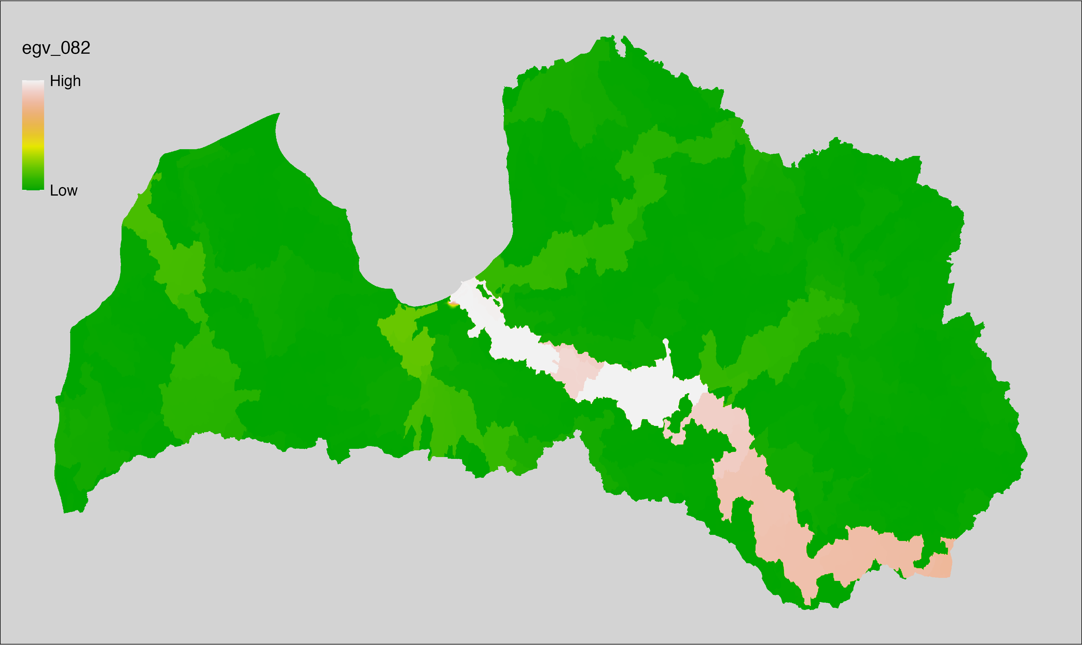
6.83 HydroClim_14-max_cell
filename: HydroClim_14-max_cell.tif
layername: egv_083
English name: Maximum per subcatchment upstream precipitation amount (kg m⁻² year⁻¹) of the driest month (HydroClim) within the analysis cell (1 ha)
Latvian name: Sateces apakšbaseina maksimālais augšteces nokrišņu daudzums sausākajā mēnesī (kg m⁻² year⁻¹) (HydroClim) analīzes šūnā (1 ha)
Procedure: Information from the HydroClim
data - including both basin and raster layers - is used. First, basin CRS is transformed to EPSG:3059. Then,
zonal statistics (per basin) using a layer specific summary function (max) are
calculated (exactextractr::exact_extract()), and the the results are rasterised with the workflow
egvtools::polygon2input(). Once rasterised to input data, EGV is created using the workflow
egvtools::input2egv(). To prevent from gaps at the edges, inverse distance
weighted (power = 2) gap filling is implemented. To save disk space,
the intermediate input layer is unlinked. Finally, the layer is standardised by
subtracting the arithmetic mean and dividing by the root mean squared error.
Code
# libs ----
if(!require(egvtools)) {remotes::install_github("aavotins/egvtools"); require(egvtools)}
if(!require(terra)) {install.packages("terra"); require(terra)}
if(!require(tidyverse)) {install.packages("tidyverse"); require(tidyverse)}
if(!require(sf)) {install.packages("sf"); require(sf)}
if(!require(sfarrow)) {install.packages("sfarrow"); require(sfarrow)}
if(!require(exactextractr)) {install.packages("exactextractr"); require(exactextractr)}
# basins ----
level12=st_read("./Geodata/2024/HydroClim/hybas_lake_eu_lev01-12_v1c/hybas_lake_eu_lev12_v1c.shp")
grid_1km=sfarrow::st_read_parquet("./Templates/TemplateGrids/tikls1km_sauzeme.parquet")
grid_1km=st_transform(grid_1km,crs=3059)
level12=st_transform(level12,crs=3059)
level12=level12[grid_1km,,]
level12=st_make_valid(level12)
# job ----
localname="HydroClim_14-max_cell.tif"
layername="egv_083"
summary_function="max"
slanis=rast(paste0("./Geodata/2024/HydroClim/",localname))
level12$Hydro_values=exact_extract(slanis,level12,fun=summary_function)
polygon2input(vector_data = level12,
template_path = "./Templates/TemplateRasters/LV10m_10km.tif",
out_path = "./RasterGrids_10m/2024/",
file_name = localname,
value_field = "Hydro_values",
fun="first",
value_type = "continuous",
prepare=FALSE,
project_mode = "auto",
check_na = FALSE,
plot_result=FALSE,
plot_gaps = FALSE,
overwrite=TRUE)
egvrez=input2egv(input=paste0("./RasterGrids_10m/2024/",localname),
egv_template= "./Templates/TemplateRasters/LV100m_10km.tif",
summary_function = "average",
missing_job = "FillOutput",
input_template = "./Templates/TemplateRasters/LV10m_10km.tif",
outlocation = "./RasterGrids_100m/2024/RAW/",
outfilename = localname,
layername = layername,
idw_weight = 2,
plot_gaps = FALSE,plot_final = FALSE)
egvrez
unlink(paste0("./RasterGrids_10m/2024/",localname))
# standardisation ----
if(!require(terra)) {install.packages("terra"); require(terra)}
if(!require(tidyverse)) {install.packages("tidyverse"); require(tidyverse)}
nosaukums="HydroClim_14-max_cell.tif"
ielasisanas_cels=paste0("./RasterGrids_100m/2024/RAW/",nosaukums)
saglabasanas_cels=paste0("./RasterGrids_100m/2024/Scaled/",nosaukums)
slanis=rast(ielasisanas_cels)
videjais=global(slanis,fun="mean",na.rm=TRUE)
centrets=slanis-videjais[,1]
standartnovirze=terra::global(centrets,fun="rms",na.rm=TRUE)
merogots=centrets/standartnovirze[,1]
writeRaster(merogots,
filename=saglabasanas_cels,
overwrite=TRUE)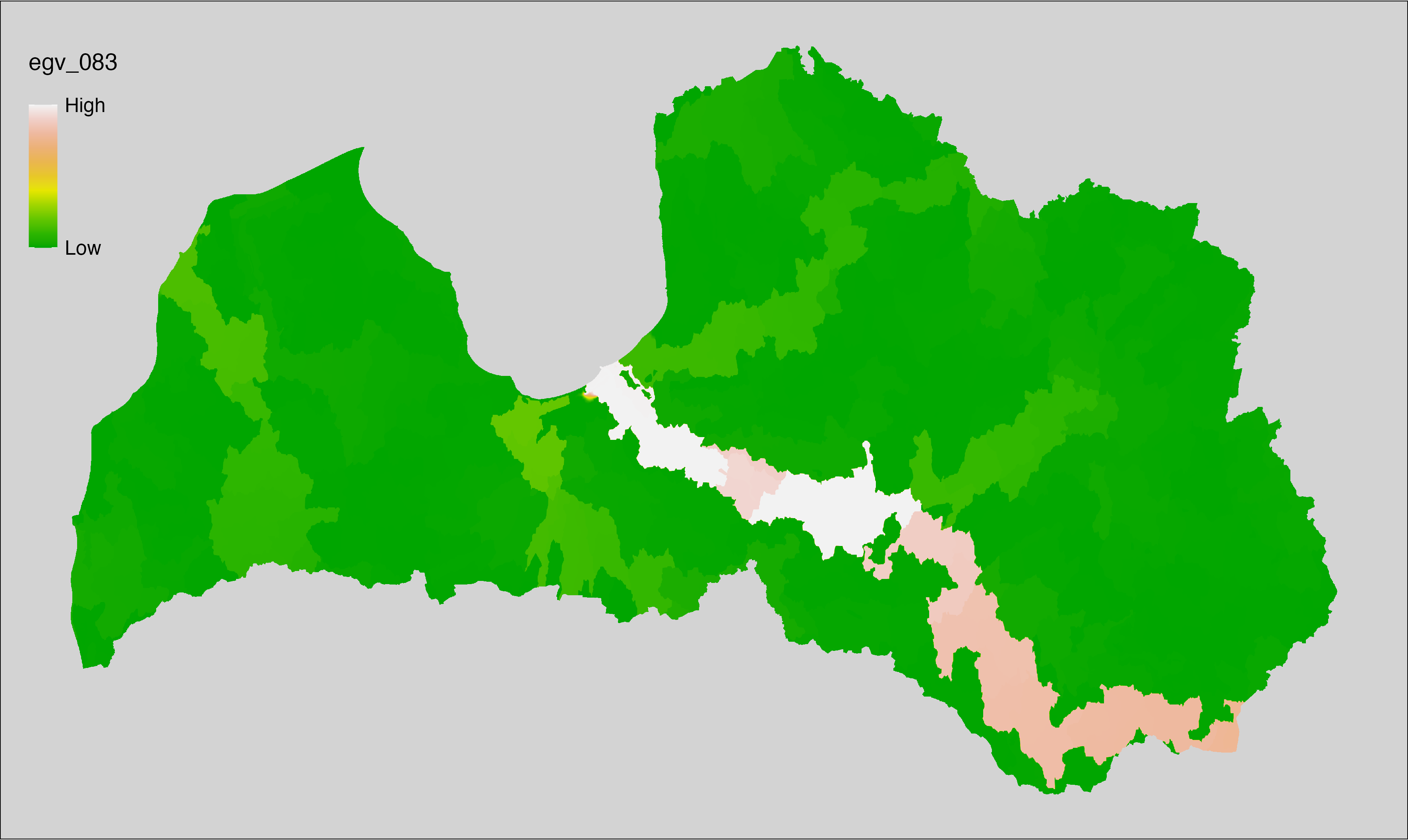
6.84 HydroClim_15-max_cell
filename: HydroClim_15-max_cell.tif
layername: egv_084
English name: Maximum per subcatchment upstream precipitation seasonality (kg m⁻²) (HydroClim) within the analysis cell (1 ha)
Latvian name: Sateces apakšbaseina maksimālais augšteces nokrišņu daudzuma sezonalitāte (kg m⁻²) (HydroClim) analīzes šūnā (1 ha)
Procedure: Information from the HydroClim
data - including both basin and raster layers - is used. First, basin CRS is transformed to EPSG:3059. Then,
zonal statistics (per basin) using a layer specific summary function (max) are
calculated (exactextractr::exact_extract()), and the the results are rasterised with the workflow
egvtools::polygon2input(). Once rasterised to input data, EGV is created using the workflow
egvtools::input2egv(). To prevent from gaps at the edges, inverse distance
weighted (power = 2) gap filling is implemented. To save disk space,
the intermediate input layer is unlinked. Finally, the layer is standardised by
subtracting the arithmetic mean and dividing by the root mean squared error.
Code
# libs ----
if(!require(egvtools)) {remotes::install_github("aavotins/egvtools"); require(egvtools)}
if(!require(terra)) {install.packages("terra"); require(terra)}
if(!require(tidyverse)) {install.packages("tidyverse"); require(tidyverse)}
if(!require(sf)) {install.packages("sf"); require(sf)}
if(!require(sfarrow)) {install.packages("sfarrow"); require(sfarrow)}
if(!require(exactextractr)) {install.packages("exactextractr"); require(exactextractr)}
# basins ----
level12=st_read("./Geodata/2024/HydroClim/hybas_lake_eu_lev01-12_v1c/hybas_lake_eu_lev12_v1c.shp")
grid_1km=sfarrow::st_read_parquet("./Templates/TemplateGrids/tikls1km_sauzeme.parquet")
grid_1km=st_transform(grid_1km,crs=3059)
level12=st_transform(level12,crs=3059)
level12=level12[grid_1km,,]
level12=st_make_valid(level12)
# job ----
localname="HydroClim_15-max_cell.tif"
layername="egv_084"
summary_function="max"
slanis=rast(paste0("./Geodata/2024/HydroClim/",localname))
level12$Hydro_values=exact_extract(slanis,level12,fun=summary_function)
polygon2input(vector_data = level12,
template_path = "./Templates/TemplateRasters/LV10m_10km.tif",
out_path = "./RasterGrids_10m/2024/",
file_name = localname,
value_field = "Hydro_values",
fun="first",
value_type = "continuous",
prepare=FALSE,
project_mode = "auto",
check_na = FALSE,
plot_result=FALSE,
plot_gaps = FALSE,
overwrite=TRUE)
egvrez=input2egv(input=paste0("./RasterGrids_10m/2024/",localname),
egv_template= "./Templates/TemplateRasters/LV100m_10km.tif",
summary_function = "average",
missing_job = "FillOutput",
input_template = "./Templates/TemplateRasters/LV10m_10km.tif",
outlocation = "./RasterGrids_100m/2024/RAW/",
outfilename = localname,
layername = layername,
idw_weight = 2,
plot_gaps = FALSE,plot_final = FALSE)
egvrez
unlink(paste0("./RasterGrids_10m/2024/",localname))
# standardisation ----
if(!require(terra)) {install.packages("terra"); require(terra)}
if(!require(tidyverse)) {install.packages("tidyverse"); require(tidyverse)}
nosaukums="HydroClim_15-max_cell.tif"
ielasisanas_cels=paste0("./RasterGrids_100m/2024/RAW/",nosaukums)
saglabasanas_cels=paste0("./RasterGrids_100m/2024/Scaled/",nosaukums)
slanis=rast(ielasisanas_cels)
videjais=global(slanis,fun="mean",na.rm=TRUE)
centrets=slanis-videjais[,1]
standartnovirze=terra::global(centrets,fun="rms",na.rm=TRUE)
merogots=centrets/standartnovirze[,1]
writeRaster(merogots,
filename=saglabasanas_cels,
overwrite=TRUE)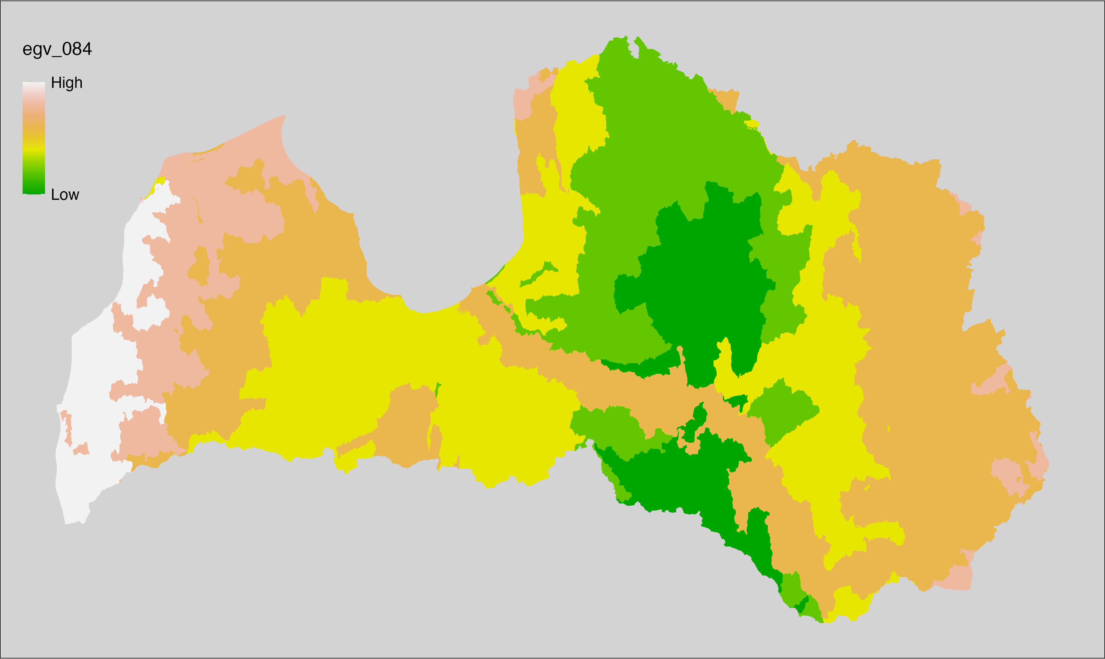
6.85 HydroClim_16-max_cell
filename: HydroClim_16-max_cell.tif
layername: egv_085
English name: Maximum per subcatchment upstream mean monthly precipitation amount (kg m⁻² year⁻¹) of the wettest quarter (HydroClim) within the analysis cell (1 ha)
Latvian name: Sateces apakšbaseina maksimālais augšteces mēneša vidējais nokrišņu daudzums mitrākajā ceturksnī (kg m⁻² year⁻¹) (HydroClim) analīzes šūnā (1 ha)
Procedure: Information from the HydroClim
data - including both basin and raster layers - is used. First, basin CRS is transformed to EPSG:3059. Then,
zonal statistics (per basin) using a layer specific summary function (max) are
calculated (exactextractr::exact_extract()), and the the results are rasterised with the workflow
egvtools::polygon2input(). Once rasterised to input data, EGV is created using the workflow
egvtools::input2egv(). To prevent from gaps at the edges, inverse distance
weighted (power = 2) gap filling is implemented. To save disk space,
the intermediate input layer is unlinked. Finally, the layer is standardised by
subtracting the arithmetic mean and dividing by the root mean squared error.
Code
# libs ----
if(!require(egvtools)) {remotes::install_github("aavotins/egvtools"); require(egvtools)}
if(!require(terra)) {install.packages("terra"); require(terra)}
if(!require(tidyverse)) {install.packages("tidyverse"); require(tidyverse)}
if(!require(sf)) {install.packages("sf"); require(sf)}
if(!require(sfarrow)) {install.packages("sfarrow"); require(sfarrow)}
if(!require(exactextractr)) {install.packages("exactextractr"); require(exactextractr)}
# basins ----
level12=st_read("./Geodata/2024/HydroClim/hybas_lake_eu_lev01-12_v1c/hybas_lake_eu_lev12_v1c.shp")
grid_1km=sfarrow::st_read_parquet("./Templates/TemplateGrids/tikls1km_sauzeme.parquet")
grid_1km=st_transform(grid_1km,crs=3059)
level12=st_transform(level12,crs=3059)
level12=level12[grid_1km,,]
level12=st_make_valid(level12)
# job ----
localname="HydroClim_16-max_cell.tif"
layername="egv_085"
summary_function="max"
slanis=rast(paste0("./Geodata/2024/HydroClim/",localname))
level12$Hydro_values=exact_extract(slanis,level12,fun=summary_function)
polygon2input(vector_data = level12,
template_path = "./Templates/TemplateRasters/LV10m_10km.tif",
out_path = "./RasterGrids_10m/2024/",
file_name = localname,
value_field = "Hydro_values",
fun="first",
value_type = "continuous",
prepare=FALSE,
project_mode = "auto",
check_na = FALSE,
plot_result=FALSE,
plot_gaps = FALSE,
overwrite=TRUE)
egvrez=input2egv(input=paste0("./RasterGrids_10m/2024/",localname),
egv_template= "./Templates/TemplateRasters/LV100m_10km.tif",
summary_function = "average",
missing_job = "FillOutput",
input_template = "./Templates/TemplateRasters/LV10m_10km.tif",
outlocation = "./RasterGrids_100m/2024/RAW/",
outfilename = localname,
layername = layername,
idw_weight = 2,
plot_gaps = FALSE,plot_final = FALSE)
egvrez
unlink(paste0("./RasterGrids_10m/2024/",localname))
# standardisation ----
if(!require(terra)) {install.packages("terra"); require(terra)}
if(!require(tidyverse)) {install.packages("tidyverse"); require(tidyverse)}
nosaukums="HydroClim_16-max_cell.tif"
ielasisanas_cels=paste0("./RasterGrids_100m/2024/RAW/",nosaukums)
saglabasanas_cels=paste0("./RasterGrids_100m/2024/Scaled/",nosaukums)
slanis=rast(ielasisanas_cels)
videjais=global(slanis,fun="mean",na.rm=TRUE)
centrets=slanis-videjais[,1]
standartnovirze=terra::global(centrets,fun="rms",na.rm=TRUE)
merogots=centrets/standartnovirze[,1]
writeRaster(merogots,
filename=saglabasanas_cels,
overwrite=TRUE)
6.86 HydroClim_17-max_cell
filename: HydroClim_17-max_cell.tif
layername: egv_086
English name: Maximum per subcatchment upstream mean monthly precipitation amount (kg m⁻² year⁻¹) of the driest quarter (HydroClim) within the analysis cell (1 ha)
Latvian name: Sateces apakšbaseina maksimālais augšteces mēneša vidējais nokrišņu daudzums sausākajā ceturksnī (kg m⁻² year⁻¹) (HydroClim) analīzes šūnā (1 ha)
Procedure: Information from the HydroClim
data - including both basin and raster layers - is used. First, basin CRS is transformed to EPSG:3059. Then,
zonal statistics (per basin) using a layer specific summary function (max) are
calculated (exactextractr::exact_extract()), and the the results are rasterised with the workflow
egvtools::polygon2input(). Once rasterised to input data, EGV is created using the workflow
egvtools::input2egv(). To prevent from gaps at the edges, inverse distance
weighted (power = 2) gap filling is implemented. To save disk space,
the intermediate input layer is unlinked. Finally, the layer is standardised by
subtracting the arithmetic mean and dividing by the root mean squared error.
Code
# libs ----
if(!require(egvtools)) {remotes::install_github("aavotins/egvtools"); require(egvtools)}
if(!require(terra)) {install.packages("terra"); require(terra)}
if(!require(tidyverse)) {install.packages("tidyverse"); require(tidyverse)}
if(!require(sf)) {install.packages("sf"); require(sf)}
if(!require(sfarrow)) {install.packages("sfarrow"); require(sfarrow)}
if(!require(exactextractr)) {install.packages("exactextractr"); require(exactextractr)}
# basins ----
level12=st_read("./Geodata/2024/HydroClim/hybas_lake_eu_lev01-12_v1c/hybas_lake_eu_lev12_v1c.shp")
grid_1km=sfarrow::st_read_parquet("./Templates/TemplateGrids/tikls1km_sauzeme.parquet")
grid_1km=st_transform(grid_1km,crs=3059)
level12=st_transform(level12,crs=3059)
level12=level12[grid_1km,,]
level12=st_make_valid(level12)
# job ----
localname="HydroClim_17-max_cell.tif"
layername="egv_086"
summary_function="max"
slanis=rast(paste0("./Geodata/2024/HydroClim/",localname))
level12$Hydro_values=exact_extract(slanis,level12,fun=summary_function)
polygon2input(vector_data = level12,
template_path = "./Templates/TemplateRasters/LV10m_10km.tif",
out_path = "./RasterGrids_10m/2024/",
file_name = localname,
value_field = "Hydro_values",
fun="first",
value_type = "continuous",
prepare=FALSE,
project_mode = "auto",
check_na = FALSE,
plot_result=FALSE,
plot_gaps = FALSE,
overwrite=TRUE)
egvrez=input2egv(input=paste0("./RasterGrids_10m/2024/",localname),
egv_template= "./Templates/TemplateRasters/LV100m_10km.tif",
summary_function = "average",
missing_job = "FillOutput",
input_template = "./Templates/TemplateRasters/LV10m_10km.tif",
outlocation = "./RasterGrids_100m/2024/RAW/",
outfilename = localname,
layername = layername,
idw_weight = 2,
plot_gaps = FALSE,plot_final = FALSE)
egvrez
unlink(paste0("./RasterGrids_10m/2024/",localname))
# standardisation ----
if(!require(terra)) {install.packages("terra"); require(terra)}
if(!require(tidyverse)) {install.packages("tidyverse"); require(tidyverse)}
nosaukums="HydroClim_17-max_cell.tif"
ielasisanas_cels=paste0("./RasterGrids_100m/2024/RAW/",nosaukums)
saglabasanas_cels=paste0("./RasterGrids_100m/2024/Scaled/",nosaukums)
slanis=rast(ielasisanas_cels)
videjais=global(slanis,fun="mean",na.rm=TRUE)
centrets=slanis-videjais[,1]
standartnovirze=terra::global(centrets,fun="rms",na.rm=TRUE)
merogots=centrets/standartnovirze[,1]
writeRaster(merogots,
filename=saglabasanas_cels,
overwrite=TRUE)
6.87 HydroClim_18-max_cell
filename: HydroClim_18-max_cell.tif
layername: egv_087
English name: Maximum per subcatchment upstream mean monthly precipitation amount (kg m⁻² year⁻¹) of the warmest quarter (HydroClim) within the analysis cell (1 ha)
Latvian name: Sateces apakšbaseina maksimālais augšteces mēneša vidējais nokrišņu daudzums siltākajā ceturksnī (kg m⁻² year⁻¹) (HydroClim) analīzes šūnā (1 ha)
Procedure: Information from the HydroClim
data - including both basin and raster layers - is used. First, basin CRS is transformed to EPSG:3059. Then,
zonal statistics (per basin) using a layer specific summary function (max) are
calculated (exactextractr::exact_extract()), and the the results are rasterised with the workflow
egvtools::polygon2input(). Once rasterised to input data, EGV is created using the workflow
egvtools::input2egv(). To prevent from gaps at the edges, inverse distance
weighted (power = 2) gap filling is implemented. To save disk space,
the intermediate input layer is unlinked. Finally, the layer is standardised by
subtracting the arithmetic mean and dividing by the root mean squared error.
Code
# libs ----
if(!require(egvtools)) {remotes::install_github("aavotins/egvtools"); require(egvtools)}
if(!require(terra)) {install.packages("terra"); require(terra)}
if(!require(tidyverse)) {install.packages("tidyverse"); require(tidyverse)}
if(!require(sf)) {install.packages("sf"); require(sf)}
if(!require(sfarrow)) {install.packages("sfarrow"); require(sfarrow)}
if(!require(exactextractr)) {install.packages("exactextractr"); require(exactextractr)}
# basins ----
level12=st_read("./Geodata/2024/HydroClim/hybas_lake_eu_lev01-12_v1c/hybas_lake_eu_lev12_v1c.shp")
grid_1km=sfarrow::st_read_parquet("./Templates/TemplateGrids/tikls1km_sauzeme.parquet")
grid_1km=st_transform(grid_1km,crs=3059)
level12=st_transform(level12,crs=3059)
level12=level12[grid_1km,,]
level12=st_make_valid(level12)
# job ----
localname="HydroClim_18-max_cell.tif"
layername="egv_087"
summary_function="max"
slanis=rast(paste0("./Geodata/2024/HydroClim/",localname))
level12$Hydro_values=exact_extract(slanis,level12,fun=summary_function)
polygon2input(vector_data = level12,
template_path = "./Templates/TemplateRasters/LV10m_10km.tif",
out_path = "./RasterGrids_10m/2024/",
file_name = localname,
value_field = "Hydro_values",
fun="first",
value_type = "continuous",
prepare=FALSE,
project_mode = "auto",
check_na = FALSE,
plot_result=FALSE,
plot_gaps = FALSE,
overwrite=TRUE)
egvrez=input2egv(input=paste0("./RasterGrids_10m/2024/",localname),
egv_template= "./Templates/TemplateRasters/LV100m_10km.tif",
summary_function = "average",
missing_job = "FillOutput",
input_template = "./Templates/TemplateRasters/LV10m_10km.tif",
outlocation = "./RasterGrids_100m/2024/RAW/",
outfilename = localname,
layername = layername,
idw_weight = 2,
plot_gaps = FALSE,plot_final = FALSE)
egvrez
unlink(paste0("./RasterGrids_10m/2024/",localname))
# standardisation ----
if(!require(terra)) {install.packages("terra"); require(terra)}
if(!require(tidyverse)) {install.packages("tidyverse"); require(tidyverse)}
nosaukums="HydroClim_18-max_cell.tif"
ielasisanas_cels=paste0("./RasterGrids_100m/2024/RAW/",nosaukums)
saglabasanas_cels=paste0("./RasterGrids_100m/2024/Scaled/",nosaukums)
slanis=rast(ielasisanas_cels)
videjais=global(slanis,fun="mean",na.rm=TRUE)
centrets=slanis-videjais[,1]
standartnovirze=terra::global(centrets,fun="rms",na.rm=TRUE)
merogots=centrets/standartnovirze[,1]
writeRaster(merogots,
filename=saglabasanas_cels,
overwrite=TRUE)
6.88 HydroClim_19-max_cell
filename: HydroClim_19-max_cell.tif
layername: egv_088
English name: Maximum per subcatchment upstream mean monthly precipitation amount (kg m⁻² year⁻¹) of the coldest quarter (HydroClim) within the analysis cell (1 ha)
Latvian name: Sateces apakšbaseina maksimālais augšteces mēneša vidējais nokrišņu daudzums vēsākajā ceturksnī (kg m⁻² year⁻¹) (HydroClim) analīzes šūnā (1 ha)
Procedure: Information from the HydroClim
data - including both basin and raster layers - is used. First, basin CRS is transformed to EPSG:3059. Then,
zonal statistics (per basin) using a layer specific summary function (max) are
calculated (exactextractr::exact_extract()), and the the results are rasterised with the workflow
egvtools::polygon2input(). Once rasterised to input data, EGV is created using the workflow
egvtools::input2egv(). To prevent from gaps at the edges, inverse distance
weighted (power = 2) gap filling is implemented. To save disk space,
the intermediate input layer is unlinked. Finally, the layer is standardised by
subtracting the arithmetic mean and dividing by the root mean squared error.
Code
# libs ----
if(!require(egvtools)) {remotes::install_github("aavotins/egvtools"); require(egvtools)}
if(!require(terra)) {install.packages("terra"); require(terra)}
if(!require(tidyverse)) {install.packages("tidyverse"); require(tidyverse)}
if(!require(sf)) {install.packages("sf"); require(sf)}
if(!require(sfarrow)) {install.packages("sfarrow"); require(sfarrow)}
if(!require(exactextractr)) {install.packages("exactextractr"); require(exactextractr)}
# basins ----
level12=st_read("./Geodata/2024/HydroClim/hybas_lake_eu_lev01-12_v1c/hybas_lake_eu_lev12_v1c.shp")
grid_1km=sfarrow::st_read_parquet("./Templates/TemplateGrids/tikls1km_sauzeme.parquet")
grid_1km=st_transform(grid_1km,crs=3059)
level12=st_transform(level12,crs=3059)
level12=level12[grid_1km,,]
level12=st_make_valid(level12)
# job ----
localname="HydroClim_19-max_cell.tif"
layername="egv_088"
summary_function="max"
slanis=rast(paste0("./Geodata/2024/HydroClim/",localname))
level12$Hydro_values=exact_extract(slanis,level12,fun=summary_function)
polygon2input(vector_data = level12,
template_path = "./Templates/TemplateRasters/LV10m_10km.tif",
out_path = "./RasterGrids_10m/2024/",
file_name = localname,
value_field = "Hydro_values",
fun="first",
value_type = "continuous",
prepare=FALSE,
project_mode = "auto",
check_na = FALSE,
plot_result=FALSE,
plot_gaps = FALSE,
overwrite=TRUE)
egvrez=input2egv(input=paste0("./RasterGrids_10m/2024/",localname),
egv_template= "./Templates/TemplateRasters/LV100m_10km.tif",
summary_function = "average",
missing_job = "FillOutput",
input_template = "./Templates/TemplateRasters/LV10m_10km.tif",
outlocation = "./RasterGrids_100m/2024/RAW/",
outfilename = localname,
layername = layername,
idw_weight = 2,
plot_gaps = FALSE,plot_final = FALSE)
egvrez
unlink(paste0("./RasterGrids_10m/2024/",localname))
# standardisation ----
if(!require(terra)) {install.packages("terra"); require(terra)}
if(!require(tidyverse)) {install.packages("tidyverse"); require(tidyverse)}
nosaukums="HydroClim_19-max_cell.tif"
ielasisanas_cels=paste0("./RasterGrids_100m/2024/RAW/",nosaukums)
saglabasanas_cels=paste0("./RasterGrids_100m/2024/Scaled/",nosaukums)
slanis=rast(ielasisanas_cels)
videjais=global(slanis,fun="mean",na.rm=TRUE)
centrets=slanis-videjais[,1]
standartnovirze=terra::global(centrets,fun="rms",na.rm=TRUE)
merogots=centrets/standartnovirze[,1]
writeRaster(merogots,
filename=saglabasanas_cels,
overwrite=TRUE)
6.89 Distance_Builtup_cell
filename: Distance_Builtup_cell.tif
layername: egv_089
English name: Distance to Built-Up features, average within the analysis cell (1 ha)
Latvian name: Attālums līdz apbūvei, vidējais analīzes šūnā (1 ha)
Procedure: Derived from the Landscape classification, with class 500
reclassified as 1 and others as 0. Processed using the workflow egvtools::distance2egv(). To
prevent potential data loss at edge cells, inverse distance weighted
(power = 2) gap filling is implemented. Finally, the layer is standardised
by subtracting the arithmetic mean and dividing by the root mean squared error.
Code
# libs ----
if(!require(terra)) {install.packages("terra"); require(terra)}
if(!require(egvtools)) {remotes::install_github("aavotins/egvtools"); require(egvtools)}
# Distance_Builtup_cell.tif egv_89 ----
simple_landscape=rast("./RasterGrids_10m/2024/Ainava_vienk_mask.tif")
builtup=ifel(simple_landscape==500,1,0)
plot(builtup)
distegv=distance2egv(input = builtup,
template_egv = template100,
values_as_one = 1,
fill_gaps = TRUE, idw_weight = 2,
outlocation = "RasterGrids_100m/2024/RAW/",
outfilename = "Distance_Builtup_cell.tif",
layername = "egv_089")
distegv
plot(rast("RasterGrids_100m/2024/RAW/Distance_Builtup_cell.tif"))
rm(builtup)
rm(distegv)
# standardisation ----
if(!require(terra)) {install.packages("terra"); require(terra)}
if(!require(tidyverse)) {install.packages("tidyverse"); require(tidyverse)}
nosaukums="Distance_Builtup_cell.tif"
ielasisanas_cels=paste0("./RasterGrids_100m/2024/RAW/",nosaukums)
saglabasanas_cels=paste0("./RasterGrids_100m/2024/Scaled/",nosaukums)
slanis=rast(ielasisanas_cels)
videjais=global(slanis,fun="mean",na.rm=TRUE)
centrets=slanis-videjais[,1]
standartnovirze=terra::global(centrets,fun="rms",na.rm=TRUE)
merogots=centrets/standartnovirze[,1]
writeRaster(merogots,
filename=saglabasanas_cels,
overwrite=TRUE)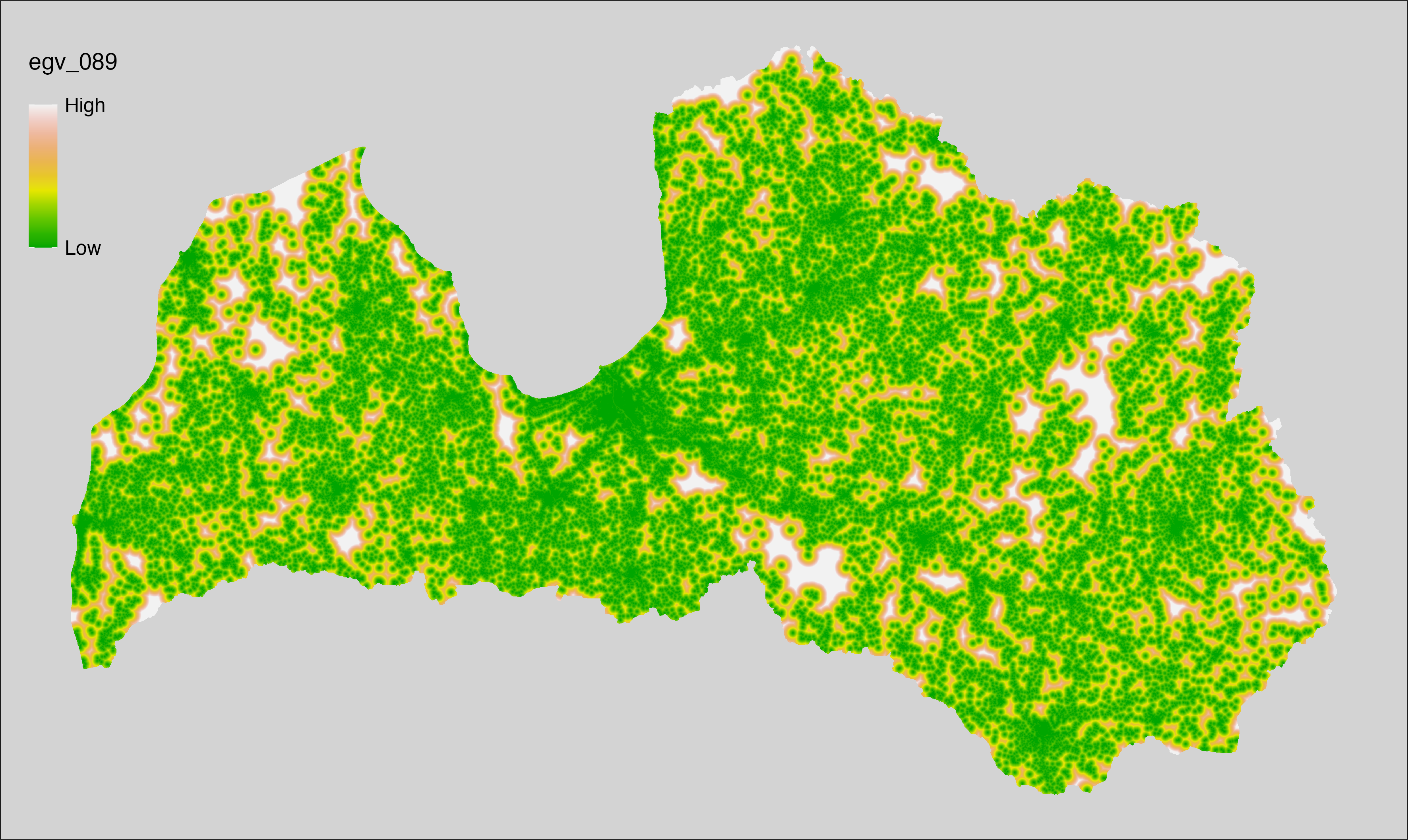
6.90 Distance_ForestInside_cell
filename: Distance_ForestInside_cell.tif
layername: egv_090
English name: Distance to Forest Edge Inside Forests, average within the analysis cell (1 ha)
Latvian name: Attālums līdz meža malai tā iekšienē, vidējais analīzes šūnā (1 ha)
Procedure: Derived from the Landscape classification, with values in
a range from 630 to 700 reclassified as 0 and others as 1. Processed
using the workflow egvtools::distance2egv(). To
prevent potential data loss at edge cells, inverse distance weighted
(power = 2) gap filling is implemented. Finally, the layer is standardised
by subtracting the arithmetic mean and dividing by the root mean squared error.
Code
# libs ----
if(!require(terra)) {install.packages("terra"); require(terra)}
if(!require(egvtools)) {remotes::install_github("aavotins/egvtools"); require(egvtools)}
# Distance_ForestInside_cell.tif egv_90 ----
simple_landscape=rast("./RasterGrids_10m/2024/Ainava_vienk_mask.tif")
trees_inside=ifel(simple_landscape>=630&simple_landscape<700,0,1)
plot(trees_inside)
distegv=distance2egv(input = trees_inside,
template_egv = template100,
values_as_one = 1,
fill_gaps = TRUE, idw_weight = 2,
outlocation = "RasterGrids_100m/2024/RAW/",
outfilename = "Distance_ForestInside_cell.tif",
layername = "egv_090")
distegv
plot(rast("RasterGrids_100m/2024/RAW/Distance_ForestInside_cell.tif"))
rm(trees_inside)
rm(distegv)
# standardisation ----
if(!require(terra)) {install.packages("terra"); require(terra)}
if(!require(tidyverse)) {install.packages("tidyverse"); require(tidyverse)}
nosaukums="Distance_ForestInside_cell.tif"
ielasisanas_cels=paste0("./RasterGrids_100m/2024/RAW/",nosaukums)
saglabasanas_cels=paste0("./RasterGrids_100m/2024/Scaled/",nosaukums)
slanis=rast(ielasisanas_cels)
videjais=global(slanis,fun="mean",na.rm=TRUE)
centrets=slanis-videjais[,1]
standartnovirze=terra::global(centrets,fun="rms",na.rm=TRUE)
merogots=centrets/standartnovirze[,1]
writeRaster(merogots,
filename=saglabasanas_cels,
overwrite=TRUE)
6.91 Distance_GrasslandPermanent_cell
filename: Distance_GrasslandPermanent_cell.tif
layername: egv_091
English name: Distance to Permanent Grasslands, average within the analysis cell (1 ha)
Latvian name: Attālums līdz ilggadīgiem zālājiem, vidējais analīzes šūnā (1 ha)
Procedure: Derived from the Rural Support Service’s information on declared
fields where PRODUCT_CODE=="710" classified as 1 and the rest of the
country as 0. Processed using the workflow egvtools::distance2egv(). To
prevent potential data loss at edge cells, inverse distance weighted
(power = 2) gap filling is implemented. Finally, the layer is standardised
by subtracting the arithmetic mean and dividing by the root mean squared error.
Code
# libs ----
if(!require(terra)) {install.packages("terra"); require(terra)}
if(!require(sf)) {install.packages("sf"); require(sf)}
if(!require(sfarrow)) {install.packages("sfarrow"); require(sfarrow)}
if(!require(tidyverse)) {install.packages("tidyverse"); require(tidyverse)}
if(!require(readxl)) {install.packages("readxl"); require(readxl)}
if(!require(raster)) {install.packages("raster"); require(raster)}
if(!require(fasterize)) {install.packages("fasterize"); require(fasterize)}
if(!require(egvtools)) {remotes::install_github("aavotins/egvtools"); require(egvtools)}
# templates ----
template10=rast("./Templates/TemplateRasters/LV10m_10km.tif")
nulls10=rast("./Templates/TemplateRasters/nulls_LV10m_10km.tif")
rastra_pamatne=raster(template10)
# Distance_GrasslandPermanent_cell.tif egv_91 ----
kodes=read_excel("./Geodata/2024/LAD/KulturuKodi_2024.xlsx")
lad=sfarrow::st_read_parquet("./Geodata/2024/LAD/Lauki_2024.parquet")
permgrass=lad %>%
filter(PRODUCT_CODE=="710") %>%
mutate(yes=1)
permgrass_r=fasterize(permgrass,rastra_pamatne,field="yes",fun="first")
permgrass_t=rast(permgrass_r)
permgrass_t2=cover(permgrass_t,nulls10)
plot(permgrass_t2)
distegv=distance2egv(input = permgrass_t2,
template_egv = template100,
values_as_one = 1,
fill_gaps = TRUE, idw_weight = 2,
outlocation = "RasterGrids_100m/2024/RAW/",
outfilename = "Distance_GrasslandPermanent_cell.tif",
layername = "egv_091")
distegv
plot(rast("RasterGrids_100m/2024/RAW/Distance_GrasslandPermanent_cell.tif"))
rm(distegv)
rm(kodes)
rm(lad)
rm(permgrass)
rm(permgrass_r)
rm(permgrass_t)
rm(permgrass_t2)
# standardisation ----
if(!require(terra)) {install.packages("terra"); require(terra)}
if(!require(tidyverse)) {install.packages("tidyverse"); require(tidyverse)}
nosaukums="Distance_GrasslandPermanent_cell.tif"
ielasisanas_cels=paste0("./RasterGrids_100m/2024/RAW/",nosaukums)
saglabasanas_cels=paste0("./RasterGrids_100m/2024/Scaled/",nosaukums)
slanis=rast(ielasisanas_cels)
videjais=global(slanis,fun="mean",na.rm=TRUE)
centrets=slanis-videjais[,1]
standartnovirze=terra::global(centrets,fun="rms",na.rm=TRUE)
merogots=centrets/standartnovirze[,1]
writeRaster(merogots,
filename=saglabasanas_cels,
overwrite=TRUE)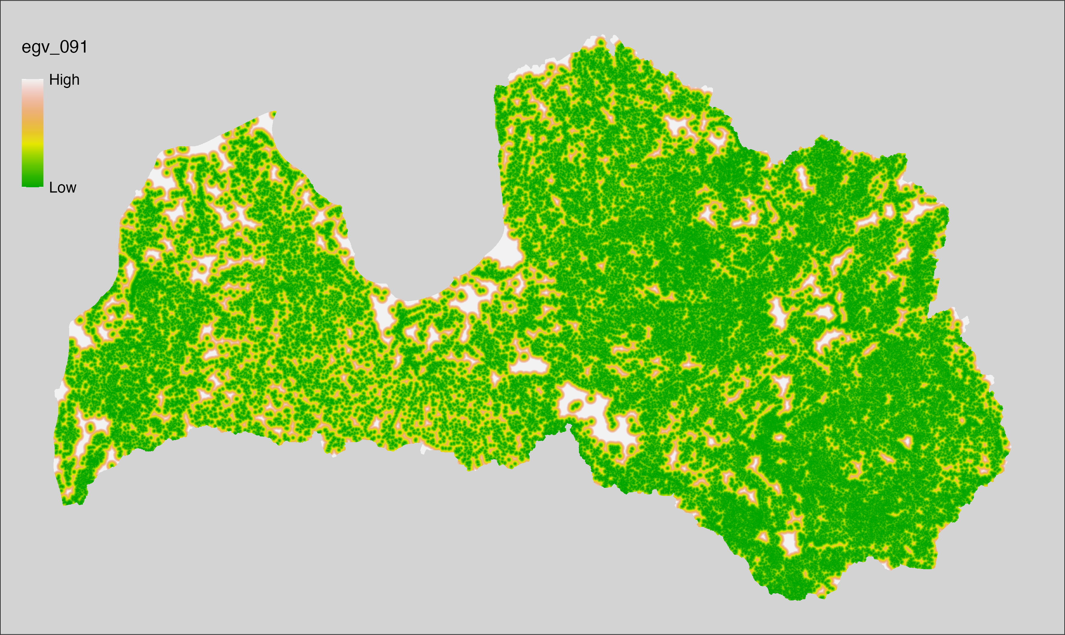
6.92 Distance_Landfill_cell
filename: Distance_Landfill_cell.tif
layername: egv_092
English name: Distance to Landfills, average within the analysis cell (1 ha)
Latvian name: Attālums līdz atkritumu poligoniem, vidējais analīzes šūnā (1 ha)
Procedure: Directly follows Waste and garbage disposal sites, landfills.
From the attachaed file, read sheet “Poligoni”;
Create an
sfobject (EPSG:3059);Rasterize and cover so that cells of interest are 1 and others are 0;
Create an EGV using the workflow
egvtools::distance2egv(). Expect warning regarding nothing to do with aggregation. This occurs becauseegvtools::distance2egv()already operate at EGV template not the input template resolution. To prevent potential data loss at edge cells, inverse distance weighted (power = 2) gap filling is implemented. Finally, the layer is standardised by subtracting the arithmetic mean and dividing by the root mean squared error.
Code
# libs ----
if(!require(terra)) {install.packages("terra"); require(terra)}
if(!require(sf)) {install.packages("sf"); require(sf)}
if(!require(tidyverse)) {install.packages("tidyverse"); require(tidyverse)}
if(!require(readxl)) {install.packages("readxl"); require(readxl)}
if(!require(egvtools)) {remotes::install_github("aavotins/egvtools"); require(egvtools)}
# templates ----
template100=rast("./Templates/TemplateRasters/LV100m_10km.tif")
nulls100=rast("./Templates/TemplateRasters/nulls_LV100m_10km.tif")
# Distance_Landfill_cell.tif egv_92 ----
# reading coordinates
landfills=read_excel("./Geodata/2024/GarbageWasteLandfills/Atkritumi.xlsx",sheet="Poligoni")
#sf object
landfills_sf=st_as_sf(landfills,coords=c("X","Y"),crs=3059)
# rasterize
landfills_rast=rasterize(landfills_sf,template100)
# raster to 1=Cell of interest, 0=background
landfills_bg=cover(landfills_rast,nulls100)
# create an egv
distegv=distance2egv(input = landfills_bg,
template_egv = template100,
values_as_one = 1,
fill_gaps = TRUE, idw_weight = 2,
outlocation = "RasterGrids_100m/2024/RAW/",
outfilename = "Distance_Landfill_cell.tif",
layername = "egv_092")
distegv
# standardisation ----
if(!require(terra)) {install.packages("terra"); require(terra)}
if(!require(tidyverse)) {install.packages("tidyverse"); require(tidyverse)}
nosaukums="Distance_Landfill_cell.tif"
ielasisanas_cels=paste0("./RasterGrids_100m/2024/RAW/",nosaukums)
saglabasanas_cels=paste0("./RasterGrids_100m/2024/Scaled/",nosaukums)
slanis=rast(ielasisanas_cels)
videjais=global(slanis,fun="mean",na.rm=TRUE)
centrets=slanis-videjais[,1]
standartnovirze=terra::global(centrets,fun="rms",na.rm=TRUE)
merogots=centrets/standartnovirze[,1]
writeRaster(merogots,
filename=saglabasanas_cels,
overwrite=TRUE)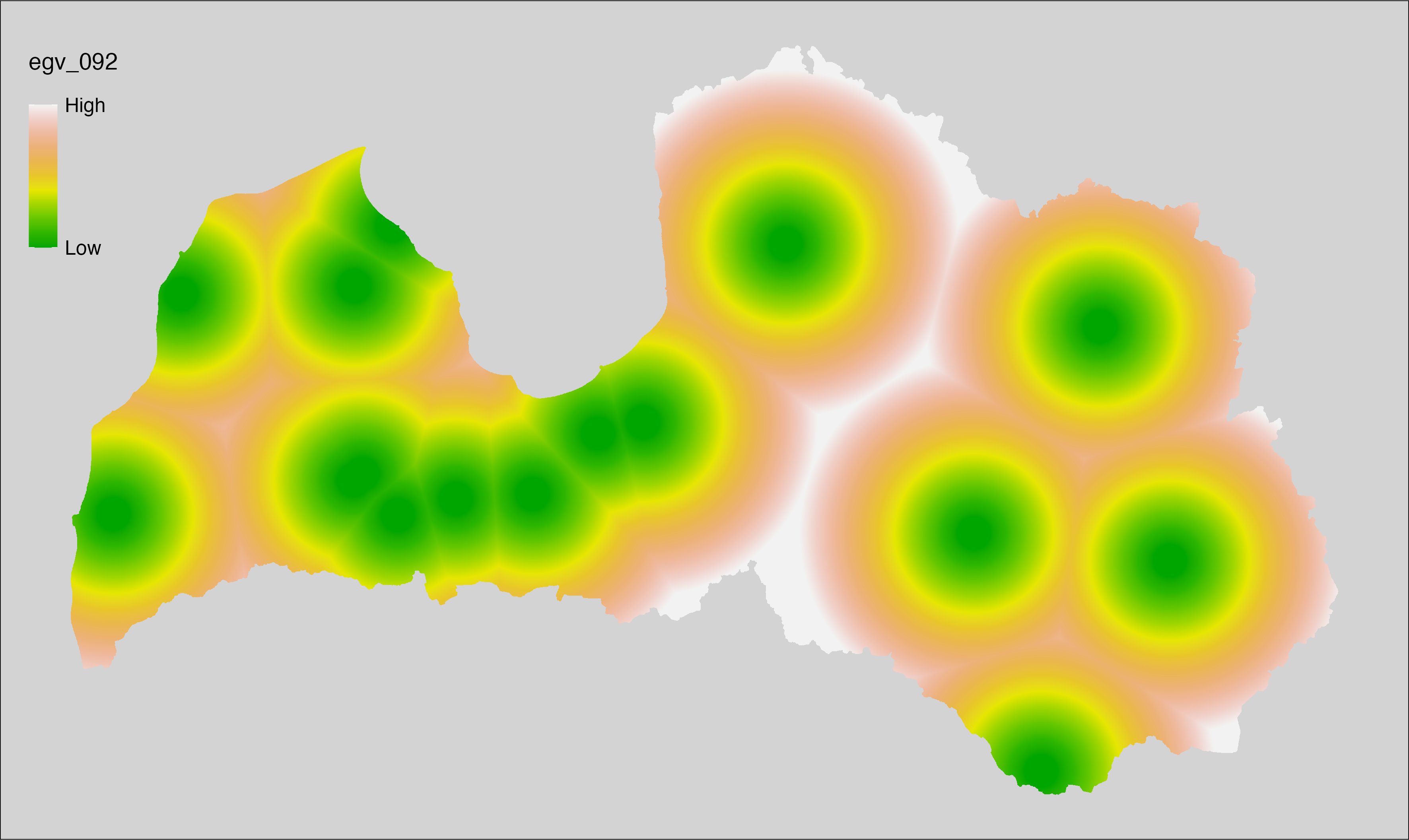
6.93 Distance_Sea_cell
filename: Distance_Sea_cell.tif
layername: egv_093
English name: Distance to Sea, average within the analysis cell (1 ha)
Latvian name: Attālums līdz jūrai, vidējais analīzes šūnā (1 ha)
Procedure: Directly follows Latvian Exclusive Economic Zone polygon.
Read layer as
sfobject (it already is EPSG:3059);Rasterize and cover so that cells of interest are 1 and others are 0;
Create an egv with the workflow
egvtools::distance2egv(). The {fasterize} package does not write CRS withWKTfrom the EPSG-string; therefore, it is better to useproject_to_template_input=TRUEand define input-template. However, the only difference is in how the CRS is stored, therefore this can ignored - distance will be calculated on the input CRS and only resulting layer will be projected to match EGV template (faster due to 10x aggregation of resolution). To protect against possible data loss at edge cells, inverse distance weighted (power = 2) gap filling is implemented. Finally, the layer is standardised by subtracting the arithmetic mean and dividing by the root mean squared error.
Code
# libs ----
if(!require(terra)) {install.packages("terra"); require(terra)}
if(!require(sf)) {install.packages("sf"); require(sf)}
if(!require(egvtools)) {remotes::install_github("aavotins/egvtools"); require(egvtools)}
if(!require(raster)) {install.packages("raster"); require(raster)}
if(!require(fasterize)) {install.packages("fasterize"); require(fasterize)}
# templates ----
template10=rast("./Templates/TemplateRasters/LV10m_10km.tif")
nulls10=rast("./Templates/TemplateRasters/nulls_LV10m_10km.tif")
rastrs10=raster::raster(template10)
# Distance_Sea_cell.tif egv_93 ----
# sea layer, sf
sea=st_read("./Geodata/2024/LV_EEZ/LV_EEZ.shp")
# quick rasterisation
sea_r=fasterize(sea,rastrs10,field="LV_EEZ")
sea_rast=rast(sea_r)
# raster to 1=Cell of interest, 0=background
sea_bg=cover(sea_rast,nulls10)
# create an egv
distegv=distance2egv(input = sea_bg,
template_egv = "./Templates/TemplateRasters/LV100m_10km.tif",
values_as_one = 1,
project_to_template_input=TRUE, # fasterize stores CRS differently
template_input=template10,
fill_gaps = TRUE, idw_weight = 2,
outlocation = "RasterGrids_100m/2024/RAW/",
outfilename = "Distance_Sea_cell.tif",
layername = "egv_093")
distegv
# standardisation ----
if(!require(terra)) {install.packages("terra"); require(terra)}
if(!require(tidyverse)) {install.packages("tidyverse"); require(tidyverse)}
nosaukums="Distance_Sea_cell.tif"
ielasisanas_cels=paste0("./RasterGrids_100m/2024/RAW/",nosaukums)
saglabasanas_cels=paste0("./RasterGrids_100m/2024/Scaled/",nosaukums)
slanis=rast(ielasisanas_cels)
videjais=global(slanis,fun="mean",na.rm=TRUE)
centrets=slanis-videjais[,1]
standartnovirze=terra::global(centrets,fun="rms",na.rm=TRUE)
merogots=centrets/standartnovirze[,1]
writeRaster(merogots,
filename=saglabasanas_cels,
overwrite=TRUE)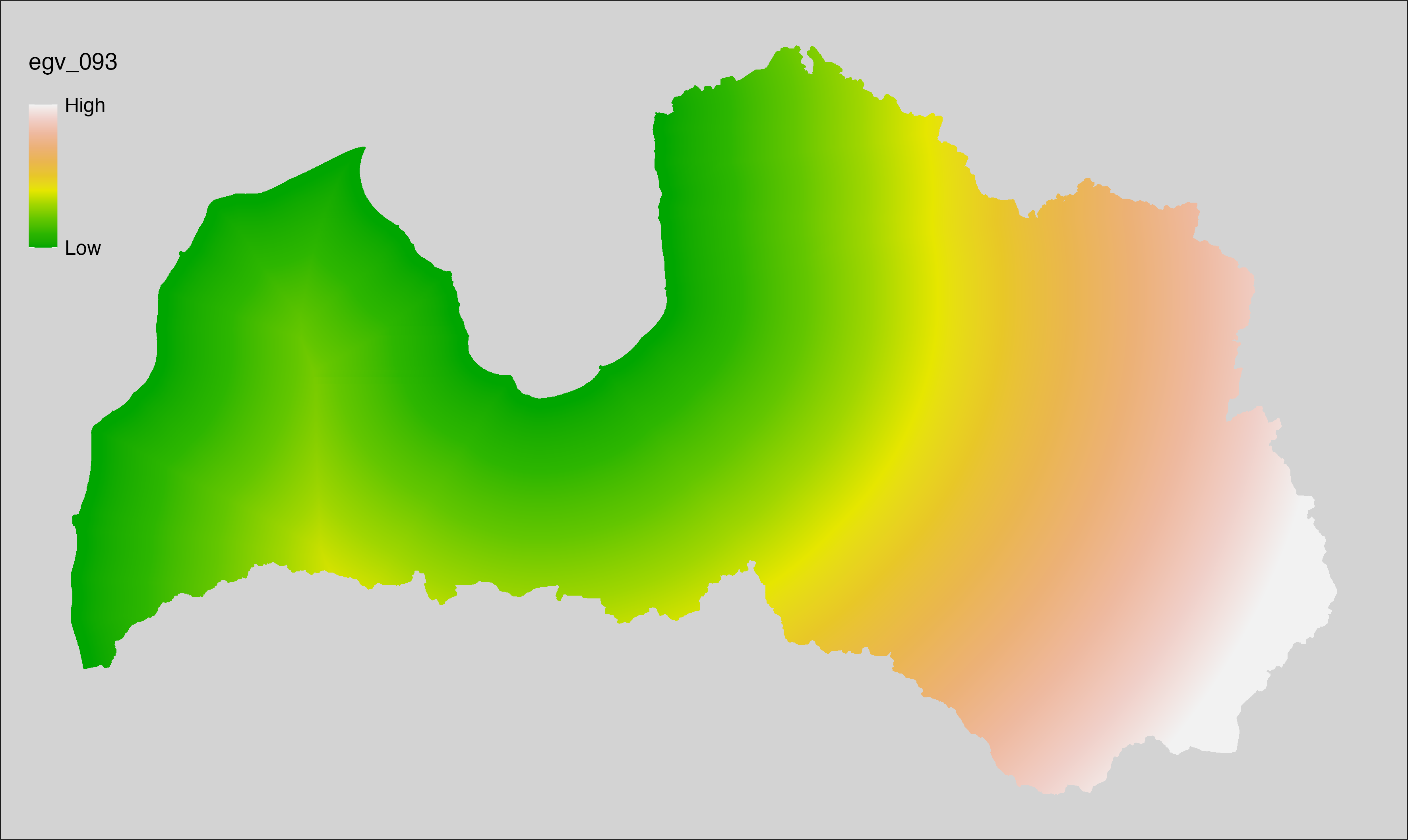
6.94 Distance_Trees_cell
filename: Distance_Trees_cell.tif
layername: egv_094
English name: Distance to Trees, average within the analysis cell (1 ha)
Latvian name: Attālums līdz kokiem, vidējais analīzes šūnā (1 ha)
Procedure: Derived from the Landscape classification, with values in
a range from 630 to 700 reclassified as 1 and all others as 0. Processed using the workflow
egvtools::distance2egv(). To prevent possible data loss at edge cells,
inverse distance weighted (power = 2) gap filling is implemented. Finally, the
layer is standardised by subtracting the arithmetic mean and dividing by the
root mean squared error.
Code
# libs ----
if(!require(terra)) {install.packages("terra"); require(terra)}
if(!require(egvtools)) {remotes::install_github("aavotins/egvtools"); require(egvtools)}
# Distance_Trees_cell.tif egv_94 ----
simple_landscape=rast("./RasterGrids_10m/2024/Ainava_vienk_mask.tif")
trees=ifel(simple_landscape>=630&simple_landscape<700,1,0)
plot(trees)
distegv=distance2egv(input = trees,
template_egv = template100,
values_as_one = 1,
fill_gaps = TRUE, idw_weight = 2,
outlocation = "RasterGrids_100m/2024/RAW/",
outfilename = "Distance_Trees_cell.tif",
layername = "egv_094")
distegv
plot(rast("RasterGrids_100m/2024/RAW/Distance_Trees_cell.tif"))
rm(trees)
rm(distegv)
# standardisation ----
if(!require(terra)) {install.packages("terra"); require(terra)}
if(!require(tidyverse)) {install.packages("tidyverse"); require(tidyverse)}
nosaukums="Distance_Trees_cell.tif"
ielasisanas_cels=paste0("./RasterGrids_100m/2024/RAW/",nosaukums)
saglabasanas_cels=paste0("./RasterGrids_100m/2024/Scaled/",nosaukums)
slanis=rast(ielasisanas_cels)
videjais=global(slanis,fun="mean",na.rm=TRUE)
centrets=slanis-videjais[,1]
standartnovirze=terra::global(centrets,fun="rms",na.rm=TRUE)
merogots=centrets/standartnovirze[,1]
writeRaster(merogots,
filename=saglabasanas_cels,
overwrite=TRUE)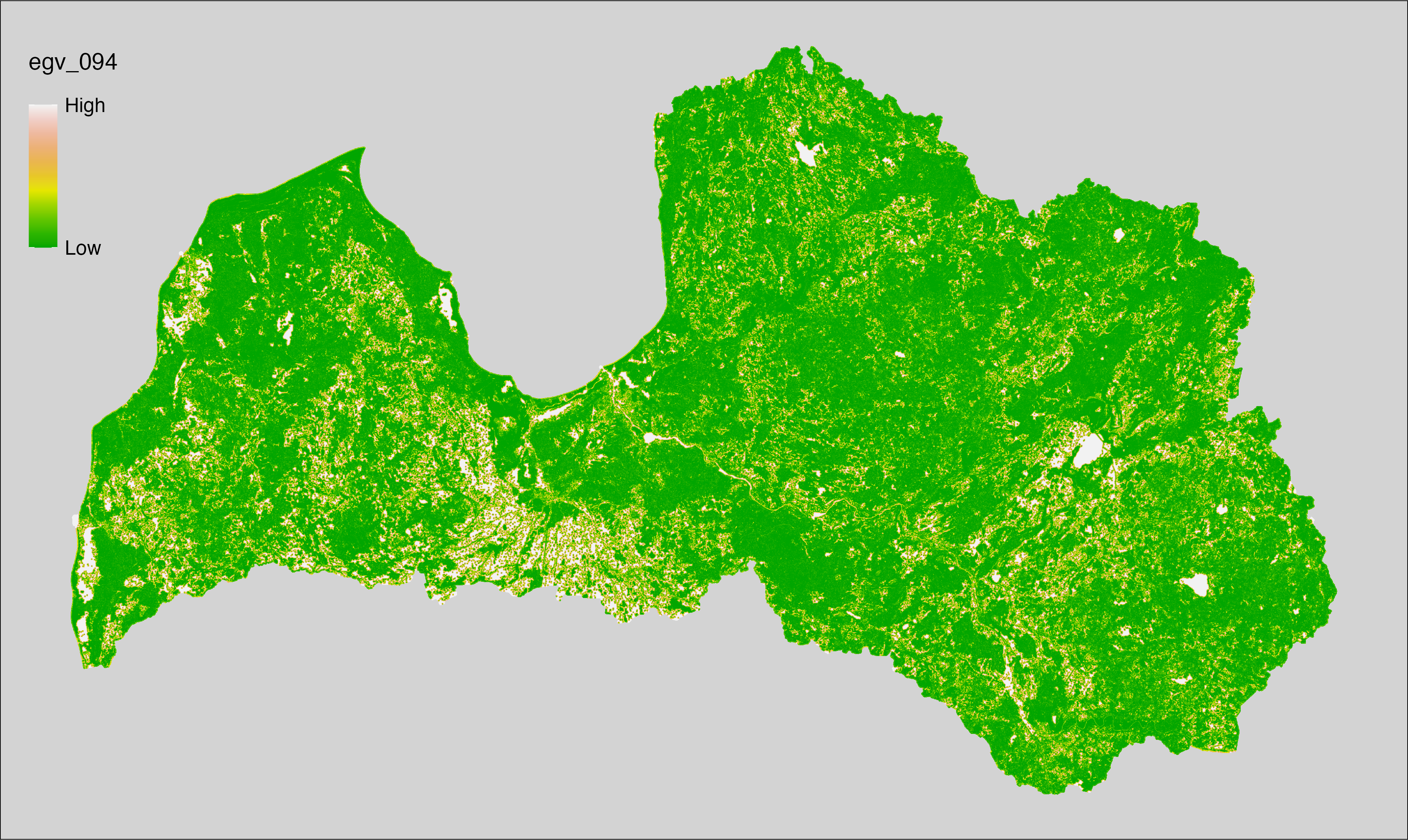
6.95 Distance_Waste_cell
filename: Distance_Waste_cell.tif
layername: egv_095
English name: Distance to Waste disposal sites, average within the analysis cell (1 ha)
Latvian name: Attālums līdz atkritumu šķirošanas un uzglabāšanas vietām, vidējais analīzes šūnā (1 ha)
Procedure: Directly follows Waste and garbage disposal sites, landfills.
From the attachaed file, read sheet “AtkritumuVietas” and clean names;
Create an
sfobject (EPSG:3059);Filter to non-deposit collection locations;
Rasterize and cover so that cells of interest are 1 and others are 0;
Create an EGV using the workflow
egvtools::distance2egv(). Expect warning regarding nothing to do with aggregation. That is becauseegvtools::distance2egv()already operate at EGV template not the input template resolution. To prevent possible data loss at edge cells, inverse distance weighted (power = 2) gap filling is implemented.Finally, the layer is standardised by subtracting the arithmetic mean and dividing by the root mean squared error.
Code
# libs ----
if(!require(terra)) {install.packages("terra"); require(terra)}
if(!require(sf)) {install.packages("sf"); require(sf)}
if(!require(tidyverse)) {install.packages("tidyverse"); require(tidyverse)}
if(!require(readxl)) {install.packages("readxl"); require(readxl)}
if(!require(egvtools)) {remotes::install_github("aavotins/egvtools"); require(egvtools)}
# templates ----
template100=rast("./Templates/TemplateRasters/LV100m_10km.tif")
nulls100=rast("./Templates/TemplateRasters/nulls_LV100m_10km.tif")
# Distance_Waste_cell.tif egv_95 ----
# reading coordinates
waste=read_excel("./Geodata/2024/GarbageWasteLandfills/Atkritumi.xlsx",sheet="AtkritumuVietas")
# cleaning names
waste2=janitor::clean_names(waste)
#sf object
waste_sf=st_as_sf(waste2,coords=c("y_koordinata_lks92_tm","x_koordinata_lks92_tm"),crs=3059)
# filtering to non-deposit
table(waste_sf$pienemsanas_vietas_tips)
waste_sf2=waste_sf %>%
filter(!str_detect(pienemsanas_vietas_tips,"Depozīta"))
# rasterize
waste_rast=rasterize(waste_sf2,template100)
# raster to 1=Cell of interest, 0=background
wastw_bg=cover(waste_rast,nulls100)
# create an egv
distegv=distance2egv(input = wastw_bg,
template_egv = template100,
values_as_one = 1,
fill_gaps = TRUE, idw_weight = 2,
outlocation = "RasterGrids_100m/2024/RAW/",
outfilename = "Distance_Waste_cell.tif",
layername = "egv_095")
distegv
# standardisation ----
if(!require(terra)) {install.packages("terra"); require(terra)}
if(!require(tidyverse)) {install.packages("tidyverse"); require(tidyverse)}
nosaukums="Distance_Waste_cell.tif"
ielasisanas_cels=paste0("./RasterGrids_100m/2024/RAW/",nosaukums)
saglabasanas_cels=paste0("./RasterGrids_100m/2024/Scaled/",nosaukums)
slanis=rast(ielasisanas_cels)
videjais=global(slanis,fun="mean",na.rm=TRUE)
centrets=slanis-videjais[,1]
standartnovirze=terra::global(centrets,fun="rms",na.rm=TRUE)
merogots=centrets/standartnovirze[,1]
writeRaster(merogots,
filename=saglabasanas_cels,
overwrite=TRUE)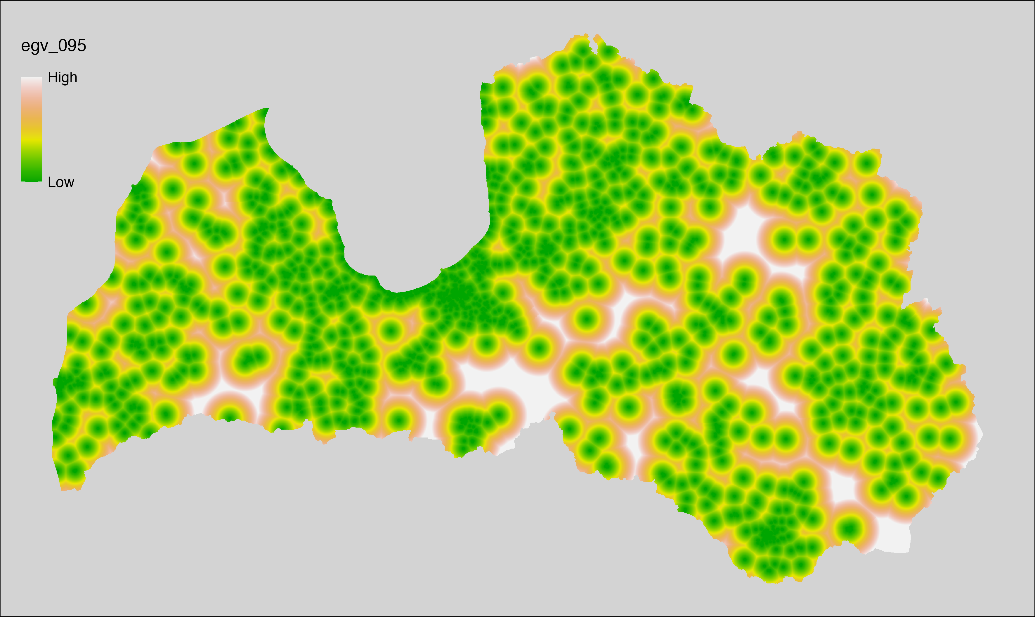
6.96 Distance_Water_cell
filename: Distance_Water_cell.tif
layername: egv_096
English name: Distance to Waterbodies, average within the analysis cell (1 ha)
Latvian name: Attālums līdz ūdenstilpēm, vidējais analīzes šūnā (1 ha)
Procedure: Derived from the Landscape classification, with class 200
reclassified as 1 and all others as 0. Processed using the workflow egvtools::distance2egv(). To
prevent possible data loss at edge cells, inverse distance weighted
(power = 2) gap filling is implemented. Finally, the layer is standardised
by subtracting the arithmetic mean and dividing by the root mean squared error.
Code
# libs ----
if(!require(terra)) {install.packages("terra"); require(terra)}
if(!require(egvtools)) {remotes::install_github("aavotins/egvtools"); require(egvtools)}
# Distance_Water_cell.tif egv_96 ----
simple_landscape=rast("./RasterGrids_10m/2024/Ainava_vienk_mask.tif")
water=ifel(simple_landscape==200,1,0)
plot(water)
distegv=distance2egv(input = water,
template_egv = template100,
values_as_one = 1,
fill_gaps = TRUE, idw_weight = 2,
outlocation = "RasterGrids_100m/2024/RAW/",
outfilename = "Distance_Water_cell.tif",
layername = "egv_096")
distegv
plot(rast("RasterGrids_100m/2024/RAW/Distance_Water_cell.tif"))
rm(water)
rm(distegv)
# standardisation ----
if(!require(terra)) {install.packages("terra"); require(terra)}
if(!require(tidyverse)) {install.packages("tidyverse"); require(tidyverse)}
nosaukums="Distance_Water_cell.tif"
ielasisanas_cels=paste0("./RasterGrids_100m/2024/RAW/",nosaukums)
saglabasanas_cels=paste0("./RasterGrids_100m/2024/Scaled/",nosaukums)
slanis=rast(ielasisanas_cels)
videjais=global(slanis,fun="mean",na.rm=TRUE)
centrets=slanis-videjais[,1]
standartnovirze=terra::global(centrets,fun="rms",na.rm=TRUE)
merogots=centrets/standartnovirze[,1]
writeRaster(merogots,
filename=saglabasanas_cels,
overwrite=TRUE)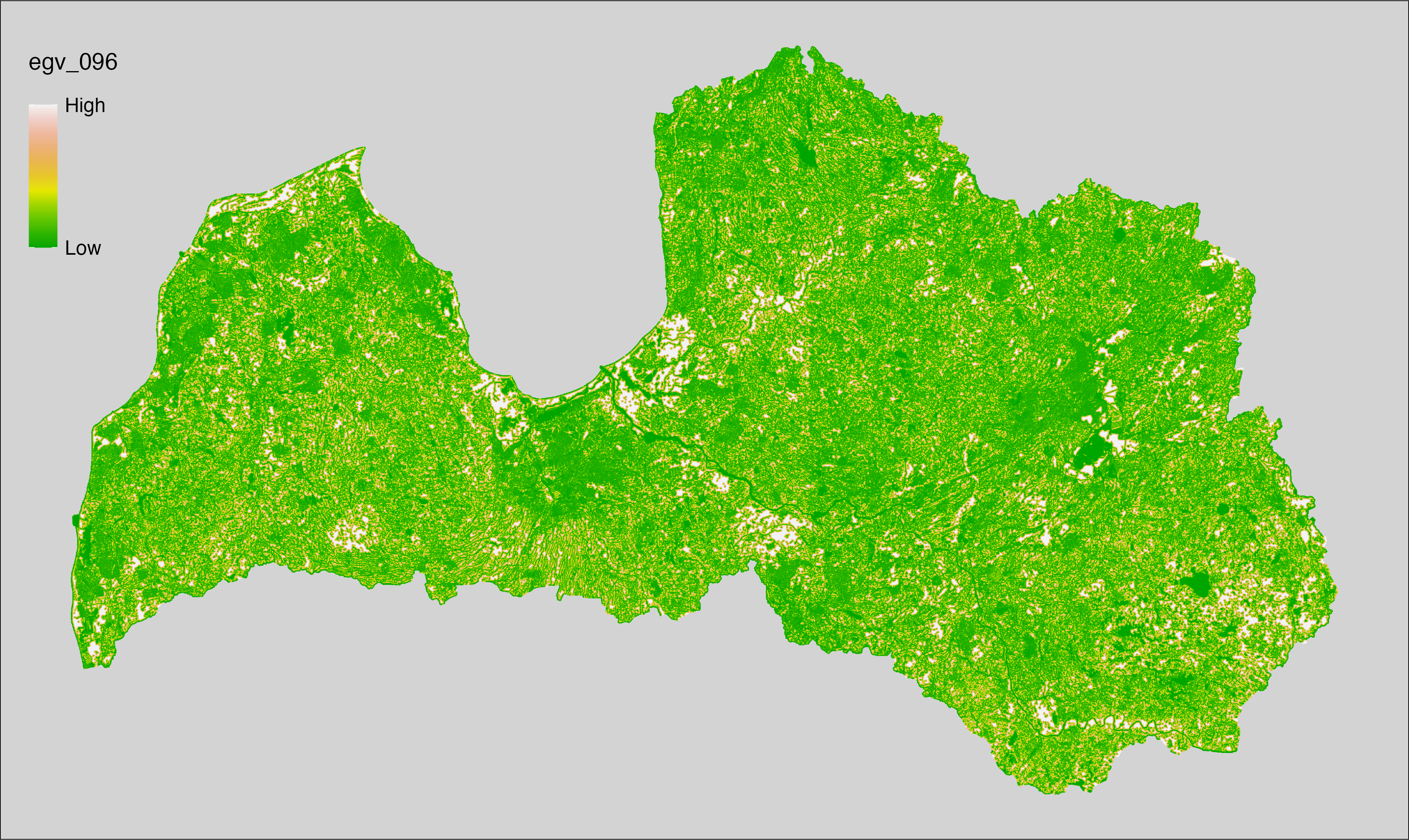
6.97 Distance_WaterInside_cell
filename: Distance_WaterInside_cell.tif
layername: egv_097
English name: Distance to Waterbody Edge Inside Waterbody, average within the analysis cell (1 ha)
Latvian name: Attālums līdz ūdenstilpes malai tās iekšienē, vidējais analīzes šūnā (1 ha)
Procedure: Derived from the Landscape classification, with class 200
reclassified as 0 and all others as 1. Processed using the workflow egvtools::distance2egv(). To
prevent possible data loss at edge cells, inverse distance weighted
(power = 2) gap filling is implemented. Finally, the layer is standardised
by subtracting the arithmetic mean and dividing by the root mean squared error.
Code
# libs ----
if(!require(terra)) {install.packages("terra"); require(terra)}
if(!require(egvtools)) {remotes::install_github("aavotins/egvtools"); require(egvtools)}
# Distance_WaterInside_cell.tif egv_97 ----
simple_landscape=rast("./RasterGrids_10m/2024/Ainava_vienk_mask.tif")
water_outside=ifel(simple_landscape==200,0,1)
plot(water_outside)
distegv=distance2egv(input = water_outside,
template_egv = template100,
values_as_one = 1,
fill_gaps = TRUE, idw_weight = 2,
outlocation = "RasterGrids_100m/2024/RAW/",
outfilename = "Distance_WaterInside_cell.tif",
layername = "egv_097")
distegv
plot(rast("RasterGrids_100m/2024/RAW/Distance_WaterInside_cell.tif"))
rm(water_outside)
rm(distegv)
# standardisation ----
if(!require(terra)) {install.packages("terra"); require(terra)}
if(!require(tidyverse)) {install.packages("tidyverse"); require(tidyverse)}
nosaukums="Distance_WaterInside_cell.tif"
ielasisanas_cels=paste0("./RasterGrids_100m/2024/RAW/",nosaukums)
saglabasanas_cels=paste0("./RasterGrids_100m/2024/Scaled/",nosaukums)
slanis=rast(ielasisanas_cels)
videjais=global(slanis,fun="mean",na.rm=TRUE)
centrets=slanis-videjais[,1]
standartnovirze=terra::global(centrets,fun="rms",na.rm=TRUE)
merogots=centrets/standartnovirze[,1]
writeRaster(merogots,
filename=saglabasanas_cels,
overwrite=TRUE)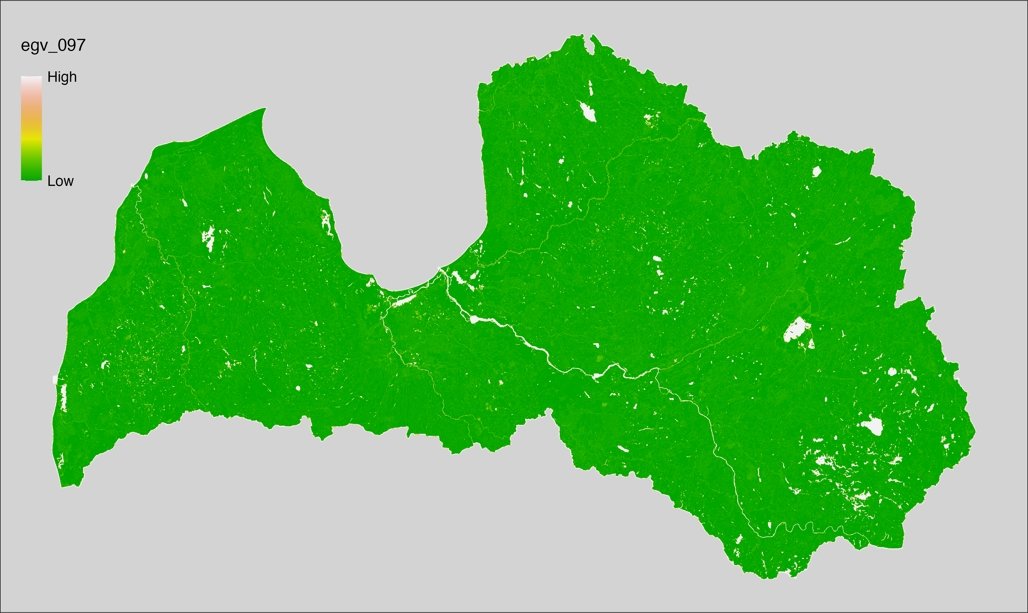
6.98 Diversity_Farmland_r500
filename: Diversity_Farmland_r500.tif
layername: egv_098
English name: Average farmland class α-diversity of 500 m grid cells within the 0.5 km landscape
Latvian name: Vidējā lauku ainavas klašu 500 m šūnu α-daudzveidība 0,5 km ainavā
Procedure: Derived from the Landscape diversity, more precisely
Farmland diversity. The average value of 25 ha cells diversity index
values is calculated using the workflow egvtools::radius_function(). To
prevent possible data loss at edge cells, inverse distance weighted
(power = 2) gap filling is implemented. File is written twice, to ensure
layername. Finally, the layer is standardised
by subtracting the arithmetic mean and dividing by the root mean squared error.
Code
# libs ----
if(!require(egvtools)) {remotes::install_github("aavotins/egvtools"); require(egvtools)}
if(!require(terra)) {install.packages("terra"); require(terra)}
# templates ----
template100=rast("./Templates/TemplateRasters/LV100m_10km.tif")
# radii
radius_function(
kvadrati_path = "./Templates/TemplateGrids/tiles/",
radii_path = "./Templates/TemplateGridPoints/tiles/",
tikls100_path = "./Templates/TemplateGrids/tikls100_sauzeme.parquet",
template_path = "./Templates/TemplateRasters/LV100m_10km.tif",
input_layers = c("./RasterGrids_500m/2024/Diversity_Farmland_500x.tif"),
layer_prefixes = c("Diversity_Farmland"),
output_dir = "./RasterGrids_100m/2024/RAW/",
n_workers = 12,
radii = c("r500"),
radius_mode = "sparse",
extract_fun = "mean",
fill_missing = TRUE,
IDW_weight = 2,
future_max_size = 5 * 1024^3)
# Diversity_Farmland_r500.tif egv_98
slanis=rast("./RasterGrids_100m/2024/RAW/Diversity_Farmland_r500.tif")
names(slanis)="egv_098"
slanis2=project(slanis,template100)
writeRaster(slanis2,
"./RasterGrids_100m/2024/RAW/Diversity_Farmland_r500.tif",
overwrite=TRUE)
# standardisation ----
if(!require(terra)) {install.packages("terra"); require(terra)}
if(!require(tidyverse)) {install.packages("tidyverse"); require(tidyverse)}
nosaukums="Diversity_Farmland_r500.tif"
ielasisanas_cels=paste0("./RasterGrids_100m/2024/RAW/",nosaukums)
saglabasanas_cels=paste0("./RasterGrids_100m/2024/Scaled/",nosaukums)
slanis=rast(ielasisanas_cels)
videjais=global(slanis,fun="mean",na.rm=TRUE)
centrets=slanis-videjais[,1]
standartnovirze=terra::global(centrets,fun="rms",na.rm=TRUE)
merogots=centrets/standartnovirze[,1]
writeRaster(merogots,
filename=saglabasanas_cels,
overwrite=TRUE)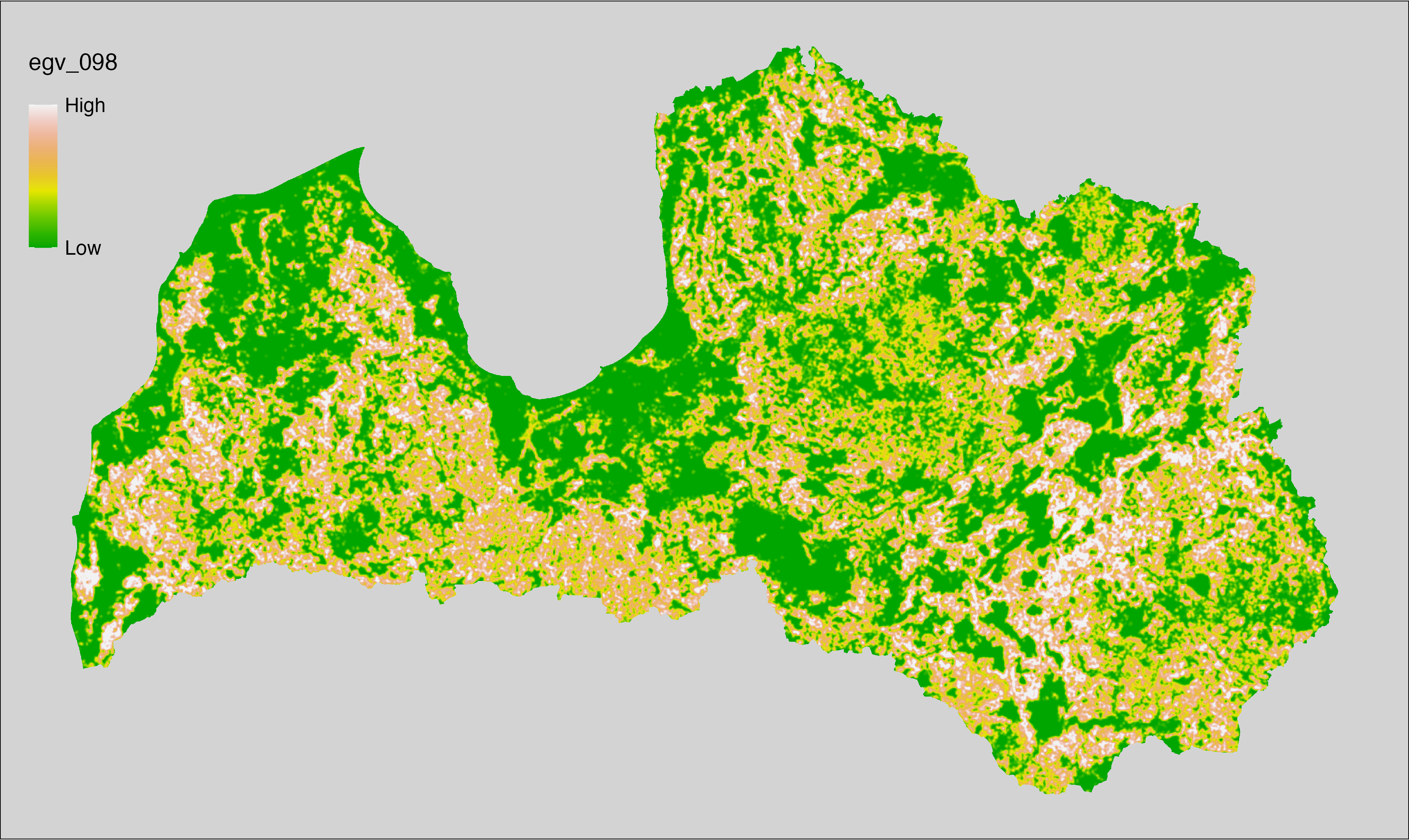
6.99 Diversity_Farmland_r1250
filename: Diversity_Farmland_r1250.tif
layername: egv_099
English name: Average farmland class α-diversity of 500 m grid cells within the 1.25 km landscape
Latvian name: Vidējā lauku ainavas klašu 500 m šūnu α-daudzveidība 1,25 km ainavā
Procedure: Derived from the Landscape diversity, more precisely
Farmland diversity. The average value of 25 ha cells diversity index
values is calculated using the workflow egvtools::radius_function(). To
prevent possible data loss at edge cells, inverse distance weighted
(power = 2) gap filling is implemented. File is written twice, to ensure
layername. Finally, the layer is standardised
by subtracting the arithmetic mean and dividing by the root mean squared error.
Code
# libs ----
if(!require(egvtools)) {remotes::install_github("aavotins/egvtools"); require(egvtools)}
if(!require(terra)) {install.packages("terra"); require(terra)}
# templates ----
template100=rast("./Templates/TemplateRasters/LV100m_10km.tif")
# radii
radius_function(
kvadrati_path = "./Templates/TemplateGrids/tiles/",
radii_path = "./Templates/TemplateGridPoints/tiles/",
tikls100_path = "./Templates/TemplateGrids/tikls100_sauzeme.parquet",
template_path = "./Templates/TemplateRasters/LV100m_10km.tif",
input_layers = c("./RasterGrids_500m/2024/Diversity_Farmland_500x.tif"),
layer_prefixes = c("Diversity_Farmland"),
output_dir = "./RasterGrids_100m/2024/RAW/",
n_workers = 12,
radii = c("r1250"),
radius_mode = "sparse",
extract_fun = "mean",
fill_missing = TRUE,
IDW_weight = 2,
future_max_size = 5 * 1024^3)
# Diversity_Farmland_r1250.tif egv_99
slanis=rast("./RasterGrids_100m/2024/RAW/Diversity_Farmland_r1250.tif")
names(slanis)="egv_099"
slanis2=project(slanis,template100)
writeRaster(slanis2,
"./RasterGrids_100m/2024/RAW/Diversity_Farmland_r1250.tif",
overwrite=TRUE)
# standardisation ----
if(!require(terra)) {install.packages("terra"); require(terra)}
if(!require(tidyverse)) {install.packages("tidyverse"); require(tidyverse)}
nosaukums="Diversity_Farmland_r1250.tif"
ielasisanas_cels=paste0("./RasterGrids_100m/2024/RAW/",nosaukums)
saglabasanas_cels=paste0("./RasterGrids_100m/2024/Scaled/",nosaukums)
slanis=rast(ielasisanas_cels)
videjais=global(slanis,fun="mean",na.rm=TRUE)
centrets=slanis-videjais[,1]
standartnovirze=terra::global(centrets,fun="rms",na.rm=TRUE)
merogots=centrets/standartnovirze[,1]
writeRaster(merogots,
filename=saglabasanas_cels,
overwrite=TRUE)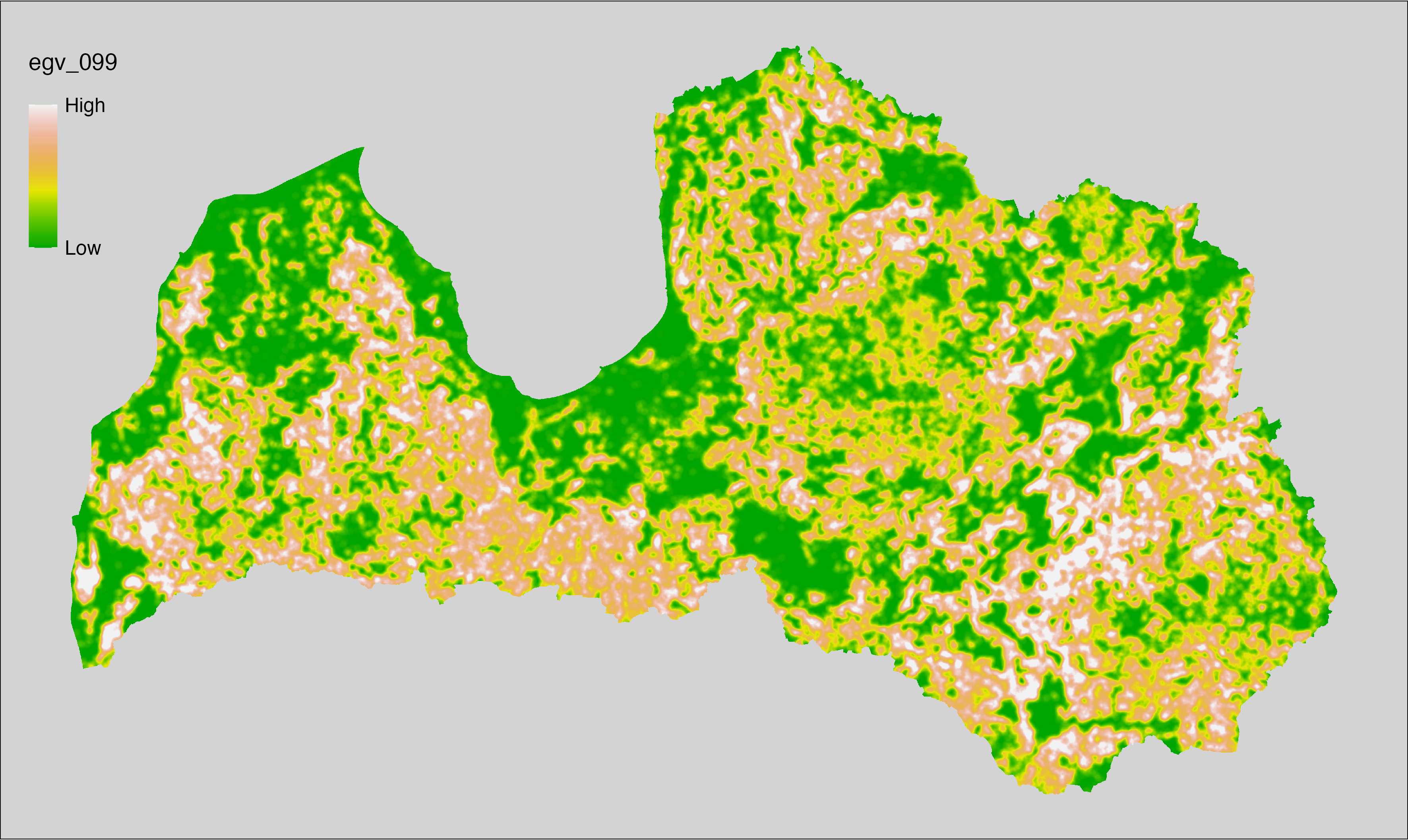
6.100 Diversity_Farmland_r3000
filename: Diversity_Farmland_r3000.tif
layername: egv_100
English name: Average farmland class α-diversity of 500 m grid cells within the 3 km landscape
Latvian name: Vidējā lauku ainavas klašu 500 m šūnu α-daudzveidība 3 km ainavā
Procedure: Derived from the Landscape diversity, more precisely
Farmland diversity. The average value of 25 ha cells diversity index
values is calculated using the workflow egvtools::radius_function(). To
prevent possible data loss at edge cells, inverse distance weighted
(power = 2) gap filling is implemented. File is written twice, to ensure
layername. Finally, the layer is standardised
by subtracting the arithmetic mean and dividing by the root mean squared error.
Code
# libs ----
if(!require(egvtools)) {remotes::install_github("aavotins/egvtools"); require(egvtools)}
if(!require(terra)) {install.packages("terra"); require(terra)}
# templates ----
template100=rast("./Templates/TemplateRasters/LV100m_10km.tif")
# radii
radius_function(
kvadrati_path = "./Templates/TemplateGrids/tiles/",
radii_path = "./Templates/TemplateGridPoints/tiles/",
tikls100_path = "./Templates/TemplateGrids/tikls100_sauzeme.parquet",
template_path = "./Templates/TemplateRasters/LV100m_10km.tif",
input_layers = c("./RasterGrids_500m/2024/Diversity_Farmland_500x.tif"),
layer_prefixes = c("Diversity_Farmland"),
output_dir = "./RasterGrids_100m/2024/RAW/",
n_workers = 12,
radii = c("r3000"),
radius_mode = "sparse",
extract_fun = "mean",
fill_missing = TRUE,
IDW_weight = 2,
future_max_size = 5 * 1024^3)
# Diversity_Farmland_r3000.tif egv_100
slanis=rast("./RasterGrids_100m/2024/RAW/Diversity_Farmland_r3000.tif")
names(slanis)="egv_100"
slanis2=project(slanis,template100)
writeRaster(slanis2,
"./RasterGrids_100m/2024/RAW/Diversity_Farmland_r3000.tif",
overwrite=TRUE)
# standardisation ----
if(!require(terra)) {install.packages("terra"); require(terra)}
if(!require(tidyverse)) {install.packages("tidyverse"); require(tidyverse)}
nosaukums="Diversity_Farmland_r3000.tif"
ielasisanas_cels=paste0("./RasterGrids_100m/2024/RAW/",nosaukums)
saglabasanas_cels=paste0("./RasterGrids_100m/2024/Scaled/",nosaukums)
slanis=rast(ielasisanas_cels)
videjais=global(slanis,fun="mean",na.rm=TRUE)
centrets=slanis-videjais[,1]
standartnovirze=terra::global(centrets,fun="rms",na.rm=TRUE)
merogots=centrets/standartnovirze[,1]
writeRaster(merogots,
filename=saglabasanas_cels,
overwrite=TRUE)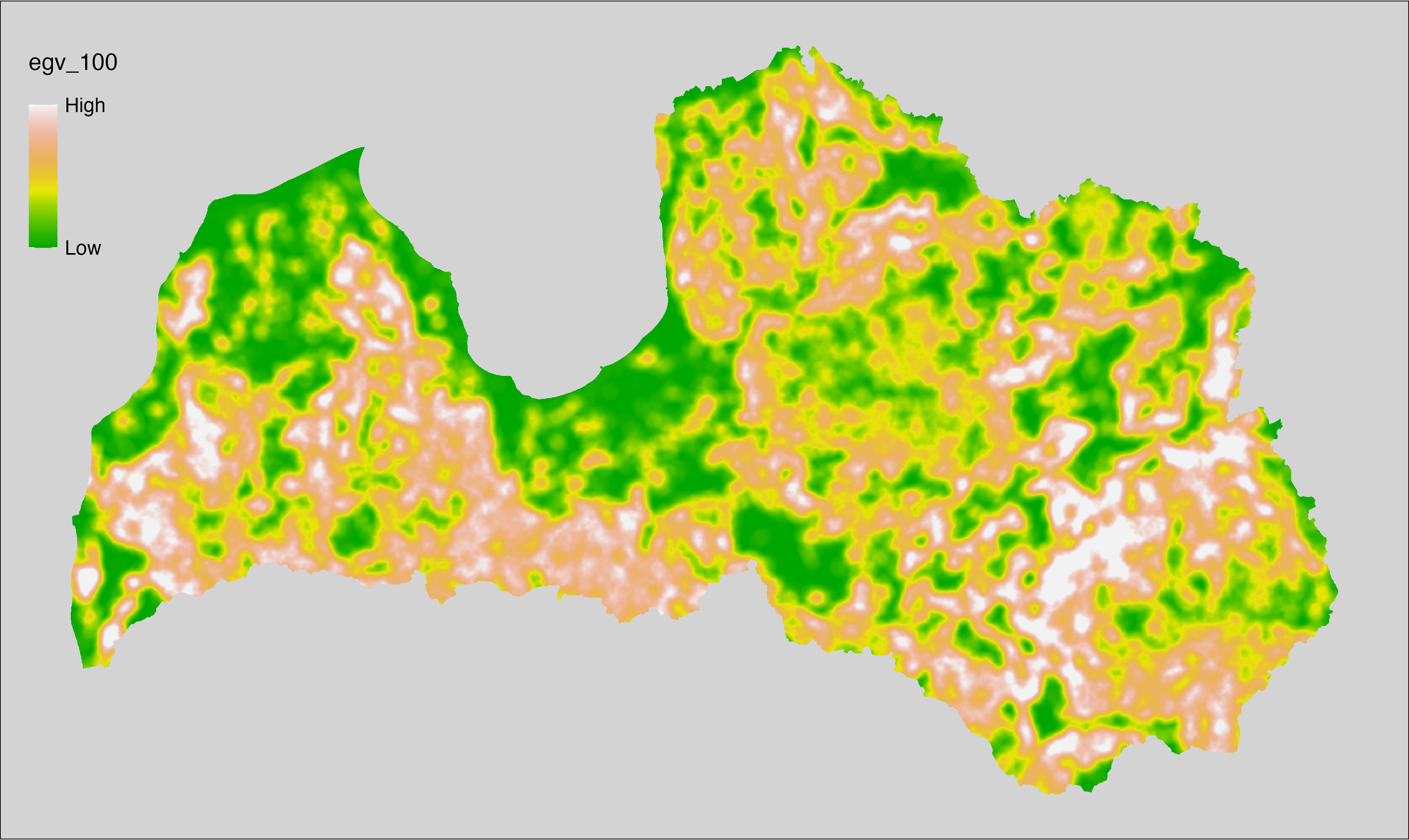
6.101 Diversity_Farmland_r10000
filename: Diversity_Farmland_r10000.tif
layername: egv_101
English name: Average farmland class α-diversity of 500 m grid cells within the 10 km landscape
Latvian name: Vidējā lauku ainavas klašu 500 m šūnu α-daudzveidība 10 km ainavā
Procedure: Derived from the Landscape diversity, more precisely
Farmland diversity. The average value of 25 ha cells diversity index
values is calculated using the workflow egvtools::radius_function(). To
prevent possible data loss at edge cells, inverse distance weighted
(power = 2) gap filling is implemented. File is written twice, to ensure
layername. Finally, the layer is standardised
by subtracting the arithmetic mean and dividing by the root mean squared error.
Code
# libs ----
if(!require(egvtools)) {remotes::install_github("aavotins/egvtools"); require(egvtools)}
if(!require(terra)) {install.packages("terra"); require(terra)}
# templates ----
template100=rast("./Templates/TemplateRasters/LV100m_10km.tif")
# radii
radius_function(
kvadrati_path = "./Templates/TemplateGrids/tiles/",
radii_path = "./Templates/TemplateGridPoints/tiles/",
tikls100_path = "./Templates/TemplateGrids/tikls100_sauzeme.parquet",
template_path = "./Templates/TemplateRasters/LV100m_10km.tif",
input_layers = c("./RasterGrids_500m/2024/Diversity_Farmland_500x.tif"),
layer_prefixes = c("Diversity_Farmland"),
output_dir = "./RasterGrids_100m/2024/RAW/",
n_workers = 12,
radii = c("r10000"),
radius_mode = "sparse",
extract_fun = "mean",
fill_missing = TRUE,
IDW_weight = 2,
future_max_size = 5 * 1024^3)
# Diversity_Farmland_r10000.tif egv_101
slanis=rast("./RasterGrids_100m/2024/RAW/Diversity_Farmland_r10000.tif")
names(slanis)="egv_101"
slanis2=project(slanis,template100)
writeRaster(slanis2,
"./RasterGrids_100m/2024/RAW/Diversity_Farmland_r10000.tif",
overwrite=TRUE)
# standardisation ----
if(!require(terra)) {install.packages("terra"); require(terra)}
if(!require(tidyverse)) {install.packages("tidyverse"); require(tidyverse)}
nosaukums="Diversity_Farmland_r10000.tif"
ielasisanas_cels=paste0("./RasterGrids_100m/2024/RAW/",nosaukums)
saglabasanas_cels=paste0("./RasterGrids_100m/2024/Scaled/",nosaukums)
slanis=rast(ielasisanas_cels)
videjais=global(slanis,fun="mean",na.rm=TRUE)
centrets=slanis-videjais[,1]
standartnovirze=terra::global(centrets,fun="rms",na.rm=TRUE)
merogots=centrets/standartnovirze[,1]
writeRaster(merogots,
filename=saglabasanas_cels,
overwrite=TRUE)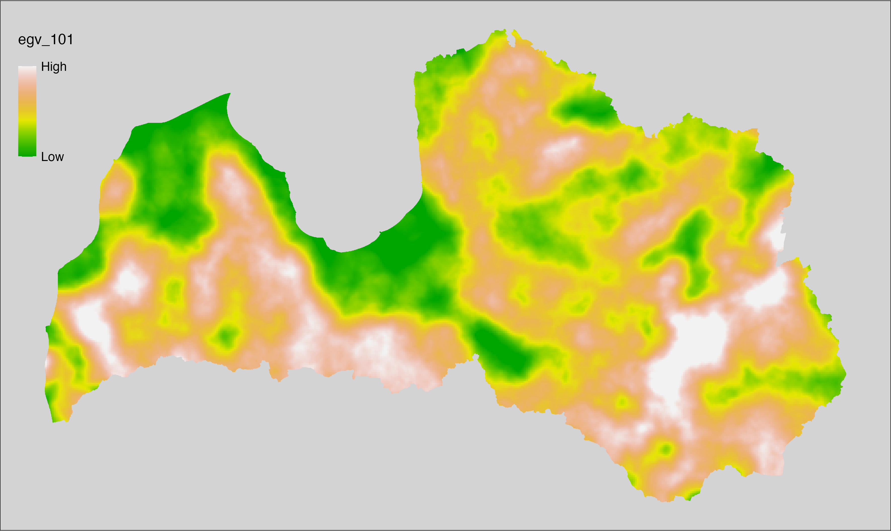
6.102 Diversity_Forest_r500
filename: Diversity_Forest_r500.tif
layername: egv_102
English name: Average forest class α-diversity of 500 m grid cells within the 0.5 km landscape
Latvian name: Vidējā mežu ainavas klašu 500 m šūnu α-daudzveidība 0,5 km ainavā
Procedure: Derived from the Landscape diversity, more precisely
Forest diversity. The average value of 25 ha cells diversity index
values is calculated using the workflow egvtools::radius_function(). To
prevent possible data loss at edge cells, inverse distance weighted
(power = 2) gap filling is implemented. File is written twice, to ensure
layername. Finally, the layer is standardised
by subtracting the arithmetic mean and dividing by the root mean squared error.
Code
# libs ----
if(!require(egvtools)) {remotes::install_github("aavotins/egvtools"); require(egvtools)}
if(!require(terra)) {install.packages("terra"); require(terra)}
# templates ----
template100=rast("./Templates/TemplateRasters/LV100m_10km.tif")
# radii
radius_function(
kvadrati_path = "./Templates/TemplateGrids/tiles/",
radii_path = "./Templates/TemplateGridPoints/tiles/",
tikls100_path = "./Templates/TemplateGrids/tikls100_sauzeme.parquet",
template_path = "./Templates/TemplateRasters/LV100m_10km.tif",
input_layers = c("./RasterGrids_500m/2024/Diversity_Forests_500x.tif"),
layer_prefixes = c("Diversity_Forest"),
output_dir = "./RasterGrids_100m/2024/RAW/",
n_workers = 12,
radii = c("r500"),
radius_mode = "sparse",
extract_fun = "mean",
fill_missing = TRUE,
IDW_weight = 2,
future_max_size = 5 * 1024^3)
# Diversity_Forest_r500.tif egv_102
slanis=rast("./RasterGrids_100m/2024/RAW/Diversity_Forest_r500.tif")
names(slanis)="egv_102"
slanis2=project(slanis,template100)
writeRaster(slanis2,
"./RasterGrids_100m/2024/RAW/Diversity_Forest_r500.tif",
overwrite=TRUE)
# standardisation ----
if(!require(terra)) {install.packages("terra"); require(terra)}
if(!require(tidyverse)) {install.packages("tidyverse"); require(tidyverse)}
nosaukums="Diversity_Forest_r500.tif"
ielasisanas_cels=paste0("./RasterGrids_100m/2024/RAW/",nosaukums)
saglabasanas_cels=paste0("./RasterGrids_100m/2024/Scaled/",nosaukums)
slanis=rast(ielasisanas_cels)
videjais=global(slanis,fun="mean",na.rm=TRUE)
centrets=slanis-videjais[,1]
standartnovirze=terra::global(centrets,fun="rms",na.rm=TRUE)
merogots=centrets/standartnovirze[,1]
writeRaster(merogots,
filename=saglabasanas_cels,
overwrite=TRUE)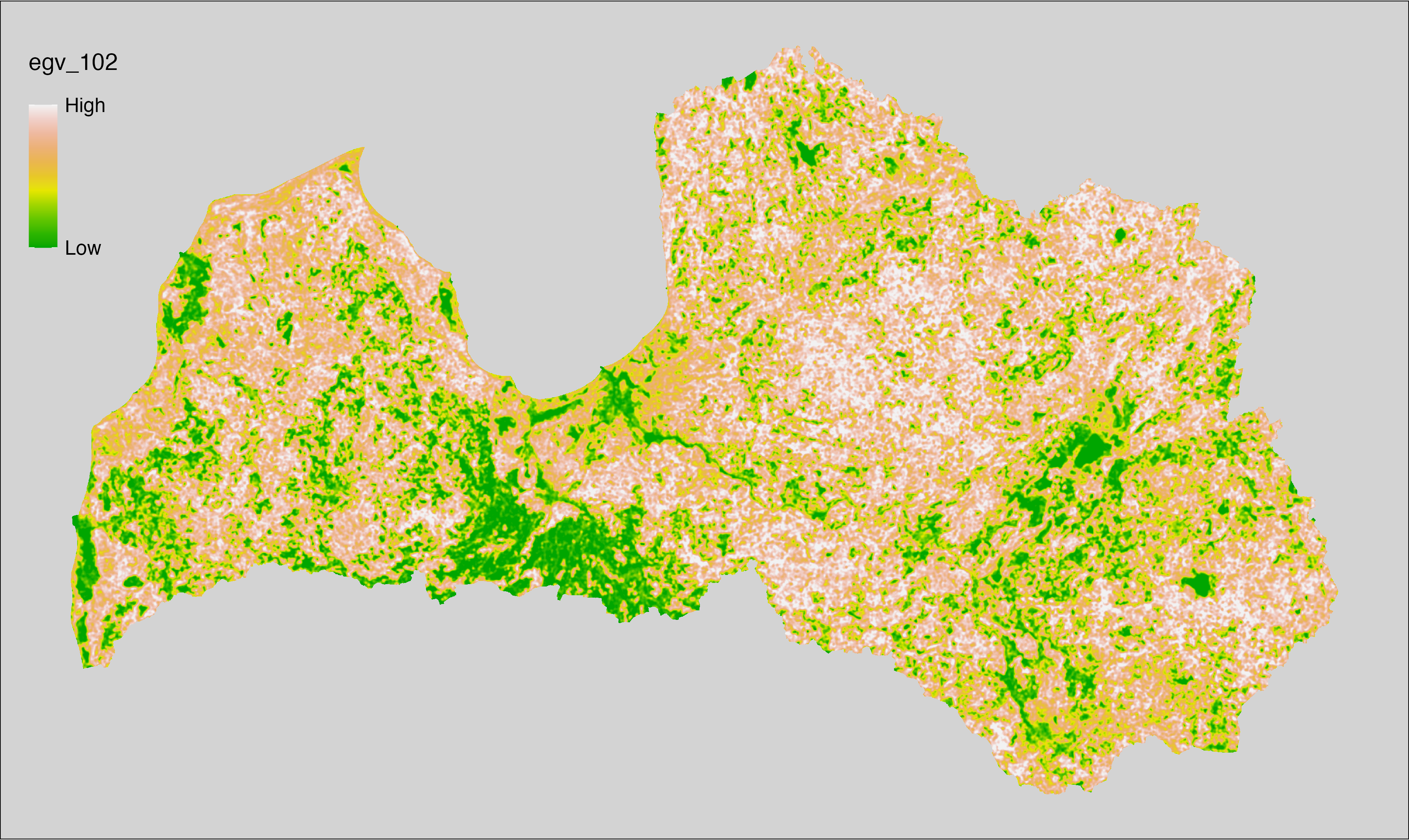
6.103 Diversity_Forest_r1250
filename: Diversity_Forest_r1250.tif
layername: egv_103
English name: Average forest class α-diversity of 500 m grid cells within the 1.25 km landscape
Latvian name: Vidējā mežu ainavas klašu 500 m šūnu α-daudzveidība 1,25 km ainavā
Procedure: Derived from the Landscape diversity, more precisely
Forest diversity. The average value of 25 ha cells diversity index
values is calculated using the workflow egvtools::radius_function(). To
prevent possible data loss at edge cells, inverse distance weighted
(power = 2) gap filling is implemented. File is written twice, to ensure
layername. Finally, the layer is standardised
by subtracting the arithmetic mean and dividing by the root mean squared error.
Code
# libs ----
if(!require(egvtools)) {remotes::install_github("aavotins/egvtools"); require(egvtools)}
if(!require(terra)) {install.packages("terra"); require(terra)}
# templates ----
template100=rast("./Templates/TemplateRasters/LV100m_10km.tif")
# radii
radius_function(
kvadrati_path = "./Templates/TemplateGrids/tiles/",
radii_path = "./Templates/TemplateGridPoints/tiles/",
tikls100_path = "./Templates/TemplateGrids/tikls100_sauzeme.parquet",
template_path = "./Templates/TemplateRasters/LV100m_10km.tif",
input_layers = c("./RasterGrids_500m/2024/Diversity_Forests_500x.tif"),
layer_prefixes = c("Diversity_Forest"),
output_dir = "./RasterGrids_100m/2024/RAW/",
n_workers = 12,
radii = c("r1250"),
radius_mode = "sparse",
extract_fun = "mean",
fill_missing = TRUE,
IDW_weight = 2,
future_max_size = 5 * 1024^3)
# Diversity_Forest_r1250.tif egv_103
slanis=rast("./RasterGrids_100m/2024/RAW/Diversity_Forest_r1250.tif")
names(slanis)="egv_103"
slanis2=project(slanis,template100)
writeRaster(slanis2,
"./RasterGrids_100m/2024/RAW/Diversity_Forest_r1250.tif",
overwrite=TRUE)
# standardisation ----
if(!require(terra)) {install.packages("terra"); require(terra)}
if(!require(tidyverse)) {install.packages("tidyverse"); require(tidyverse)}
nosaukums="Diversity_Forest_r1250.tif"
ielasisanas_cels=paste0("./RasterGrids_100m/2024/RAW/",nosaukums)
saglabasanas_cels=paste0("./RasterGrids_100m/2024/Scaled/",nosaukums)
slanis=rast(ielasisanas_cels)
videjais=global(slanis,fun="mean",na.rm=TRUE)
centrets=slanis-videjais[,1]
standartnovirze=terra::global(centrets,fun="rms",na.rm=TRUE)
merogots=centrets/standartnovirze[,1]
writeRaster(merogots,
filename=saglabasanas_cels,
overwrite=TRUE)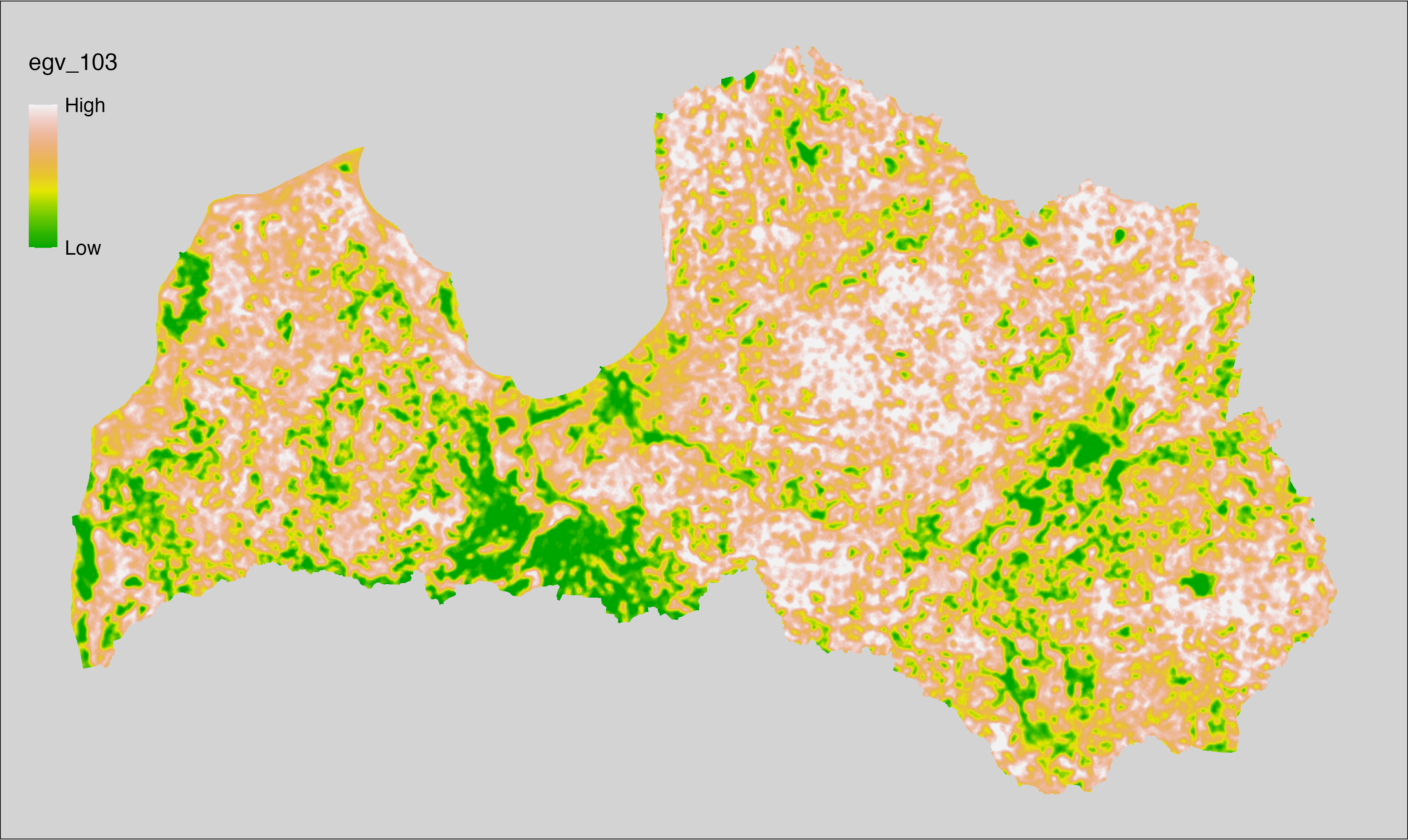
6.104 Diversity_Forest_r3000
filename: Diversity_Forest_r3000.tif
layername: egv_104
English name: Average forest class α-diversity of 500 m grid cells within the 3 km landscape
Latvian name: Vidējā mežu ainavas klašu 500 m šūnu α-daudzveidība 3 km ainavā
Procedure: Derived from the Landscape diversity, more precisely
Forest diversity. The average value of 25 ha cells diversity index
values is calculated using the workflow egvtools::radius_function(). To
prevent possible data loss at edge cells, inverse distance weighted
(power = 2) gap filling is implemented. File is written twice, to ensure
layername. Finally, the layer is standardised
by subtracting the arithmetic mean and dividing by the root mean squared error.
Code
# libs ----
if(!require(egvtools)) {remotes::install_github("aavotins/egvtools"); require(egvtools)}
if(!require(terra)) {install.packages("terra"); require(terra)}
# templates ----
template100=rast("./Templates/TemplateRasters/LV100m_10km.tif")
# radii
radius_function(
kvadrati_path = "./Templates/TemplateGrids/tiles/",
radii_path = "./Templates/TemplateGridPoints/tiles/",
tikls100_path = "./Templates/TemplateGrids/tikls100_sauzeme.parquet",
template_path = "./Templates/TemplateRasters/LV100m_10km.tif",
input_layers = c("./RasterGrids_500m/2024/Diversity_Forests_500x.tif"),
layer_prefixes = c("Diversity_Forest"),
output_dir = "./RasterGrids_100m/2024/RAW/",
n_workers = 12,
radii = c("r3000"),
radius_mode = "sparse",
extract_fun = "mean",
fill_missing = TRUE,
IDW_weight = 2,
future_max_size = 5 * 1024^3)
# Diversity_Forest_r3000.tif egv_104
slanis=rast("./RasterGrids_100m/2024/RAW/Diversity_Forest_r3000.tif")
names(slanis)="egv_104"
slanis2=project(slanis,template100)
writeRaster(slanis2,
"./RasterGrids_100m/2024/RAW/Diversity_Forest_r3000.tif",
overwrite=TRUE)
# standardisation ----
if(!require(terra)) {install.packages("terra"); require(terra)}
if(!require(tidyverse)) {install.packages("tidyverse"); require(tidyverse)}
nosaukums="Diversity_Forest_r3000.tif"
ielasisanas_cels=paste0("./RasterGrids_100m/2024/RAW/",nosaukums)
saglabasanas_cels=paste0("./RasterGrids_100m/2024/Scaled/",nosaukums)
slanis=rast(ielasisanas_cels)
videjais=global(slanis,fun="mean",na.rm=TRUE)
centrets=slanis-videjais[,1]
standartnovirze=terra::global(centrets,fun="rms",na.rm=TRUE)
merogots=centrets/standartnovirze[,1]
writeRaster(merogots,
filename=saglabasanas_cels,
overwrite=TRUE)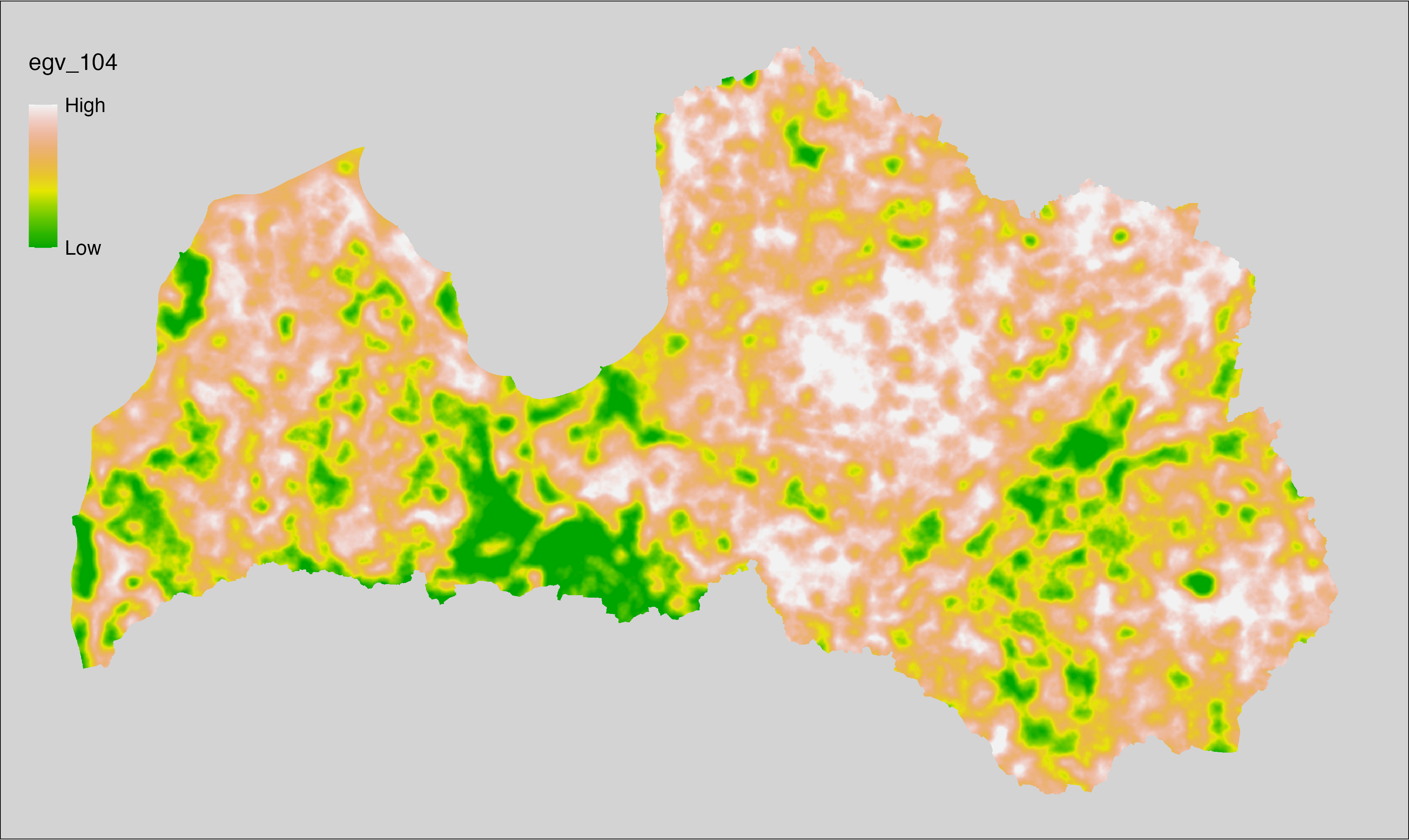
6.105 Diversity_Forest_r10000
filename: Diversity_Forest_r10000.tif
layername: egv_105
English name: Average forest class α-diversity of 500 m grid cells within the 10 km landscape
Latvian name: Vidējā mežu ainavas klašu 500 m šūnu α-daudzveidība 10 km ainavā
Procedure: Derived from the Landscape diversity, more precisely
Forest diversity. The average value of 25 ha cells diversity index
values is calculated using the workflow egvtools::radius_function(). To
prevent possible data loss at edge cells, inverse distance weighted
(power = 2) gap filling is implemented. File is written twice, to ensure
layername. Finally, the layer is standardised
by subtracting the arithmetic mean and dividing by the root mean squared error.
Code
# libs ----
if(!require(egvtools)) {remotes::install_github("aavotins/egvtools"); require(egvtools)}
if(!require(terra)) {install.packages("terra"); require(terra)}
# templates ----
template100=rast("./Templates/TemplateRasters/LV100m_10km.tif")
# radii
radius_function(
kvadrati_path = "./Templates/TemplateGrids/tiles/",
radii_path = "./Templates/TemplateGridPoints/tiles/",
tikls100_path = "./Templates/TemplateGrids/tikls100_sauzeme.parquet",
template_path = "./Templates/TemplateRasters/LV100m_10km.tif",
input_layers = c("./RasterGrids_500m/2024/Diversity_Forests_500x.tif"),
layer_prefixes = c("Diversity_Forest"),
output_dir = "./RasterGrids_100m/2024/RAW/",
n_workers = 12,
radii = c("r10000"),
radius_mode = "sparse",
extract_fun = "mean",
fill_missing = TRUE,
IDW_weight = 2,
future_max_size = 5 * 1024^3)
# Diversity_Forest_r10000.tif egv_105
slanis=rast("./RasterGrids_100m/2024/RAW/Diversity_Forest_r10000.tif")
names(slanis)="egv_105"
slanis2=project(slanis,template100)
writeRaster(slanis2,
"./RasterGrids_100m/2024/RAW/Diversity_Forest_r10000.tif",
overwrite=TRUE)
# standardisation ----
if(!require(terra)) {install.packages("terra"); require(terra)}
if(!require(tidyverse)) {install.packages("tidyverse"); require(tidyverse)}
nosaukums="Diversity_Forest_r10000.tif"
ielasisanas_cels=paste0("./RasterGrids_100m/2024/RAW/",nosaukums)
saglabasanas_cels=paste0("./RasterGrids_100m/2024/Scaled/",nosaukums)
slanis=rast(ielasisanas_cels)
videjais=global(slanis,fun="mean",na.rm=TRUE)
centrets=slanis-videjais[,1]
standartnovirze=terra::global(centrets,fun="rms",na.rm=TRUE)
merogots=centrets/standartnovirze[,1]
writeRaster(merogots,
filename=saglabasanas_cels,
overwrite=TRUE)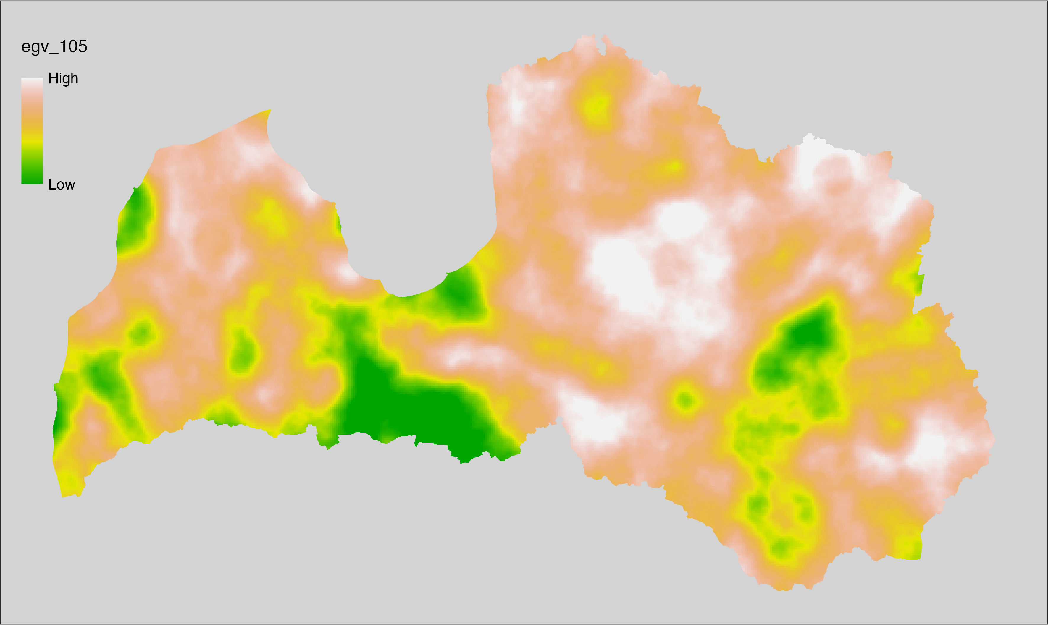
6.106 Diversity_Total_r500
filename: Diversity_Total_r500.tif
layername: egv_106
English name: Average combined landscape α-diversity of 500 m grid cells within the 0.5 km landscape
Latvian name: Vidējā visu ainavas klašu 500 m šūnu α-daudzveidība 0,5 km ainavā
Procedure: Derived from the Landscape diversity, more precisely
Overall landscape diversity. The average value of 25 ha cells diversity index
values is calculated using the workflow egvtools::radius_function(). To
prevent possible data loss at edge cells, inverse distance weighted
(power = 2) gap filling is implemented. File is written twice, to ensure
layername. Finally, the layer is standardised
by subtracting the arithmetic mean and dividing by the root mean squared error.
Code
# libs ----
if(!require(egvtools)) {remotes::install_github("aavotins/egvtools"); require(egvtools)}
if(!require(terra)) {install.packages("terra"); require(terra)}
# templates ----
template100=rast("./Templates/TemplateRasters/LV100m_10km.tif")
# radii
radius_function(
kvadrati_path = "./Templates/TemplateGrids/tiles/",
radii_path = "./Templates/TemplateGridPoints/tiles/",
tikls100_path = "./Templates/TemplateGrids/tikls100_sauzeme.parquet",
template_path = "./Templates/TemplateRasters/LV100m_10km.tif",
input_layers = c("./RasterGrids_500m/2024/Diversity_GeneralLandscape_500x.tif"),
layer_prefixes = c("Diversity_Total"),
output_dir = "./RasterGrids_100m/2024/RAW/",
n_workers = 12,
radii = c("r500"),
radius_mode = "sparse",
extract_fun = "mean",
fill_missing = TRUE,
IDW_weight = 2,
future_max_size = 5 * 1024^3)
# Diversity_Total_r500.tif egv_106
slanis=rast("./RasterGrids_100m/2024/RAW/Diversity_Total_r500.tif")
names(slanis)="egv_106"
slanis2=project(slanis,template100)
writeRaster(slanis2,
"./RasterGrids_100m/2024/RAW/Diversity_Total_r500.tif",
overwrite=TRUE)
# standardisation ----
if(!require(terra)) {install.packages("terra"); require(terra)}
if(!require(tidyverse)) {install.packages("tidyverse"); require(tidyverse)}
nosaukums="Diversity_Total_r500.tif"
ielasisanas_cels=paste0("./RasterGrids_100m/2024/RAW/",nosaukums)
saglabasanas_cels=paste0("./RasterGrids_100m/2024/Scaled/",nosaukums)
slanis=rast(ielasisanas_cels)
videjais=global(slanis,fun="mean",na.rm=TRUE)
centrets=slanis-videjais[,1]
standartnovirze=terra::global(centrets,fun="rms",na.rm=TRUE)
merogots=centrets/standartnovirze[,1]
writeRaster(merogots,
filename=saglabasanas_cels,
overwrite=TRUE)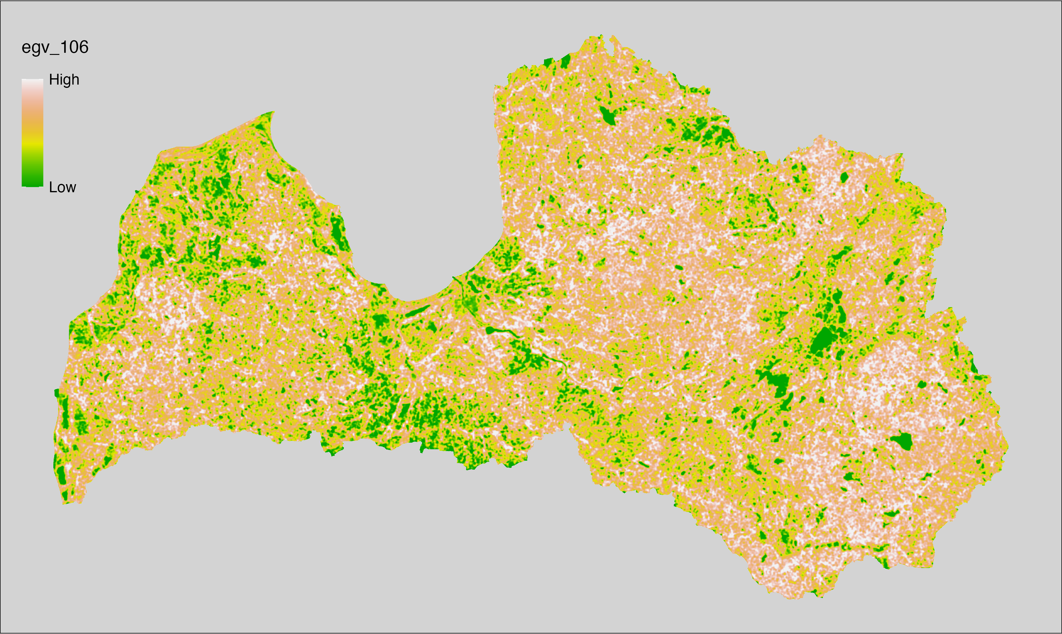
6.107 Diversity_Total_r1250
filename: Diversity_Total_r1250.tif
layername: egv_107
English name: Average combined landscape α-diversity of 500 m grid cells within the 1.25 km landscape
Latvian name: Vidējā visu ainavas klašu 500 m šūnu α-daudzveidība 1,25 km ainavā
Procedure: Derived from the Landscape diversity, more precisely
Overall landscape diversity. The average value of 25 ha cells diversity index
values is calculated using the workflow egvtools::radius_function(). To
prevent possible data loss at edge cells, inverse distance weighted
(power = 2) gap filling is implemented. File is written twice, to ensure
layername. Finally, the layer is standardised
by subtracting the arithmetic mean and dividing by the root mean squared error.
Code
# libs ----
if(!require(egvtools)) {remotes::install_github("aavotins/egvtools"); require(egvtools)}
if(!require(terra)) {install.packages("terra"); require(terra)}
# templates ----
template100=rast("./Templates/TemplateRasters/LV100m_10km.tif")
# radii
radius_function(
kvadrati_path = "./Templates/TemplateGrids/tiles/",
radii_path = "./Templates/TemplateGridPoints/tiles/",
tikls100_path = "./Templates/TemplateGrids/tikls100_sauzeme.parquet",
template_path = "./Templates/TemplateRasters/LV100m_10km.tif",
input_layers = c("./RasterGrids_500m/2024/Diversity_GeneralLandscape_500x.tif"),
layer_prefixes = c("Diversity_Total"),
output_dir = "./RasterGrids_100m/2024/RAW/",
n_workers = 12,
radii = c("r1250"),
radius_mode = "sparse",
extract_fun = "mean",
fill_missing = TRUE,
IDW_weight = 2,
future_max_size = 5 * 1024^3)
# Diversity_Total_r1250.tif egv_107
slanis=rast("./RasterGrids_100m/2024/RAW/Diversity_Total_r1250.tif")
names(slanis)="egv_107"
slanis2=project(slanis,template100)
writeRaster(slanis2,
"./RasterGrids_100m/2024/RAW/Diversity_Total_r1250.tif",
overwrite=TRUE)
# standardisation ----
if(!require(terra)) {install.packages("terra"); require(terra)}
if(!require(tidyverse)) {install.packages("tidyverse"); require(tidyverse)}
nosaukums="Diversity_Total_r1250.tif"
ielasisanas_cels=paste0("./RasterGrids_100m/2024/RAW/",nosaukums)
saglabasanas_cels=paste0("./RasterGrids_100m/2024/Scaled/",nosaukums)
slanis=rast(ielasisanas_cels)
videjais=global(slanis,fun="mean",na.rm=TRUE)
centrets=slanis-videjais[,1]
standartnovirze=terra::global(centrets,fun="rms",na.rm=TRUE)
merogots=centrets/standartnovirze[,1]
writeRaster(merogots,
filename=saglabasanas_cels,
overwrite=TRUE)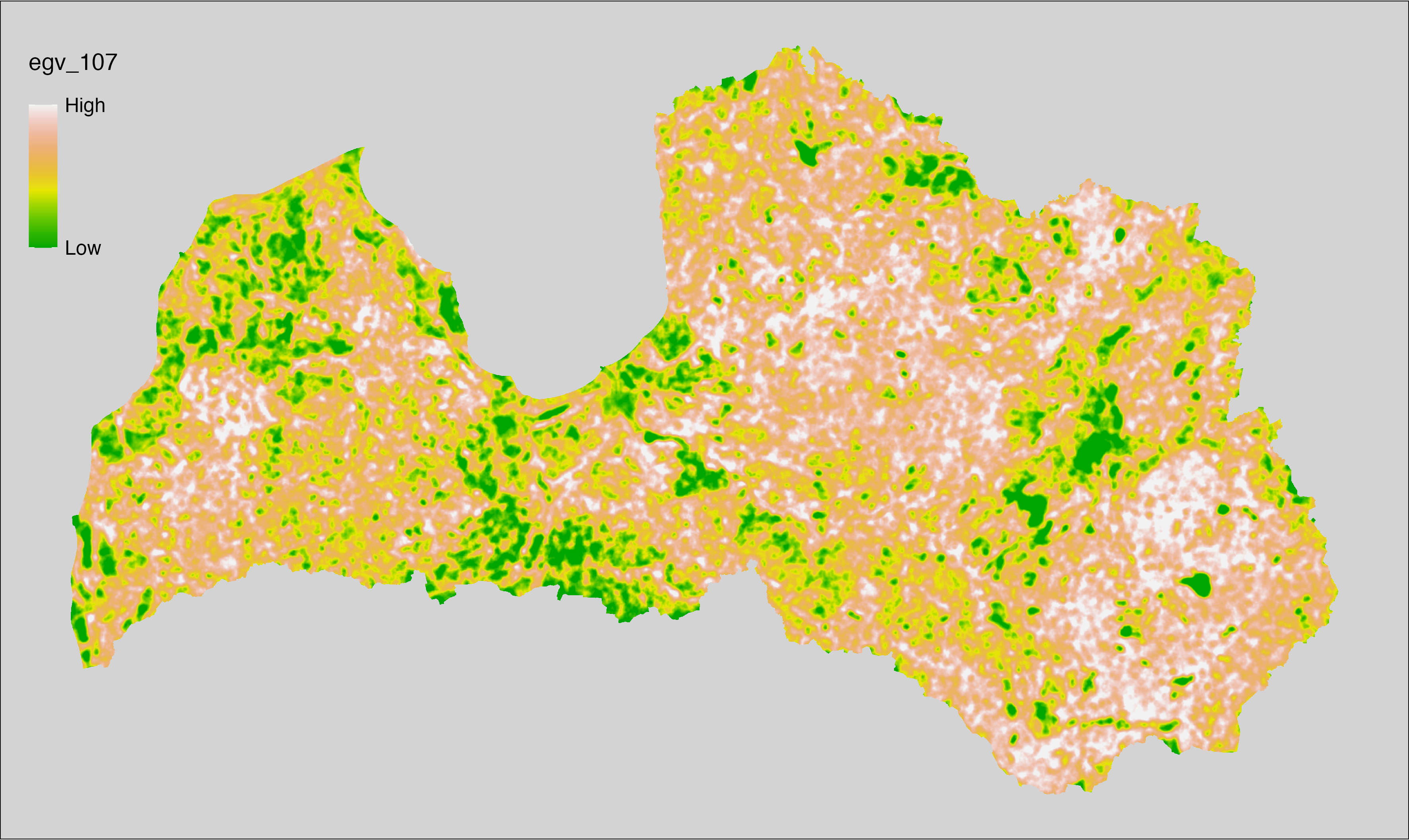
6.108 Diversity_Total_r3000
filename: Diversity_Total_r3000.tif
layername: egv_108
English name: Average combined landscape α-diversity of 500 m grid cells within the 3 km landscape
Latvian name: Vidējā visu ainavas klašu 500 m šūnu α-daudzveidība 3 km ainavā
Procedure: Derived from the Landscape diversity, more precisely
Overall landscape diversity. The average value of 25 ha cells diversity index
values is calculated using the workflow egvtools::radius_function(). To
prevent possible data loss at edge cells, inverse distance weighted
(power = 2) gap filling is implemented. File is written twice, to ensure
layername. Finally, the layer is standardised
by subtracting the arithmetic mean and dividing by the root mean squared error.
Code
# libs ----
if(!require(egvtools)) {remotes::install_github("aavotins/egvtools"); require(egvtools)}
if(!require(terra)) {install.packages("terra"); require(terra)}
# templates ----
template100=rast("./Templates/TemplateRasters/LV100m_10km.tif")
# radii
radius_function(
kvadrati_path = "./Templates/TemplateGrids/tiles/",
radii_path = "./Templates/TemplateGridPoints/tiles/",
tikls100_path = "./Templates/TemplateGrids/tikls100_sauzeme.parquet",
template_path = "./Templates/TemplateRasters/LV100m_10km.tif",
input_layers = c("./RasterGrids_500m/2024/Diversity_GeneralLandscape_500x.tif"),
layer_prefixes = c("Diversity_Total"),
output_dir = "./RasterGrids_100m/2024/RAW/",
n_workers = 12,
radii = c("r3000"),
radius_mode = "sparse",
extract_fun = "mean",
fill_missing = TRUE,
IDW_weight = 2,
future_max_size = 5 * 1024^3)
# Diversity_Total_r3000.tif egv_108
slanis=rast("./RasterGrids_100m/2024/RAW/Diversity_Total_r3000.tif")
names(slanis)="egv_108"
slanis2=project(slanis,template100)
writeRaster(slanis2,
"./RasterGrids_100m/2024/RAW/Diversity_Total_r3000.tif",
overwrite=TRUE)
# standardisation ----
if(!require(terra)) {install.packages("terra"); require(terra)}
if(!require(tidyverse)) {install.packages("tidyverse"); require(tidyverse)}
nosaukums="Diversity_Total_r3000.tif"
ielasisanas_cels=paste0("./RasterGrids_100m/2024/RAW/",nosaukums)
saglabasanas_cels=paste0("./RasterGrids_100m/2024/Scaled/",nosaukums)
slanis=rast(ielasisanas_cels)
videjais=global(slanis,fun="mean",na.rm=TRUE)
centrets=slanis-videjais[,1]
standartnovirze=terra::global(centrets,fun="rms",na.rm=TRUE)
merogots=centrets/standartnovirze[,1]
writeRaster(merogots,
filename=saglabasanas_cels,
overwrite=TRUE)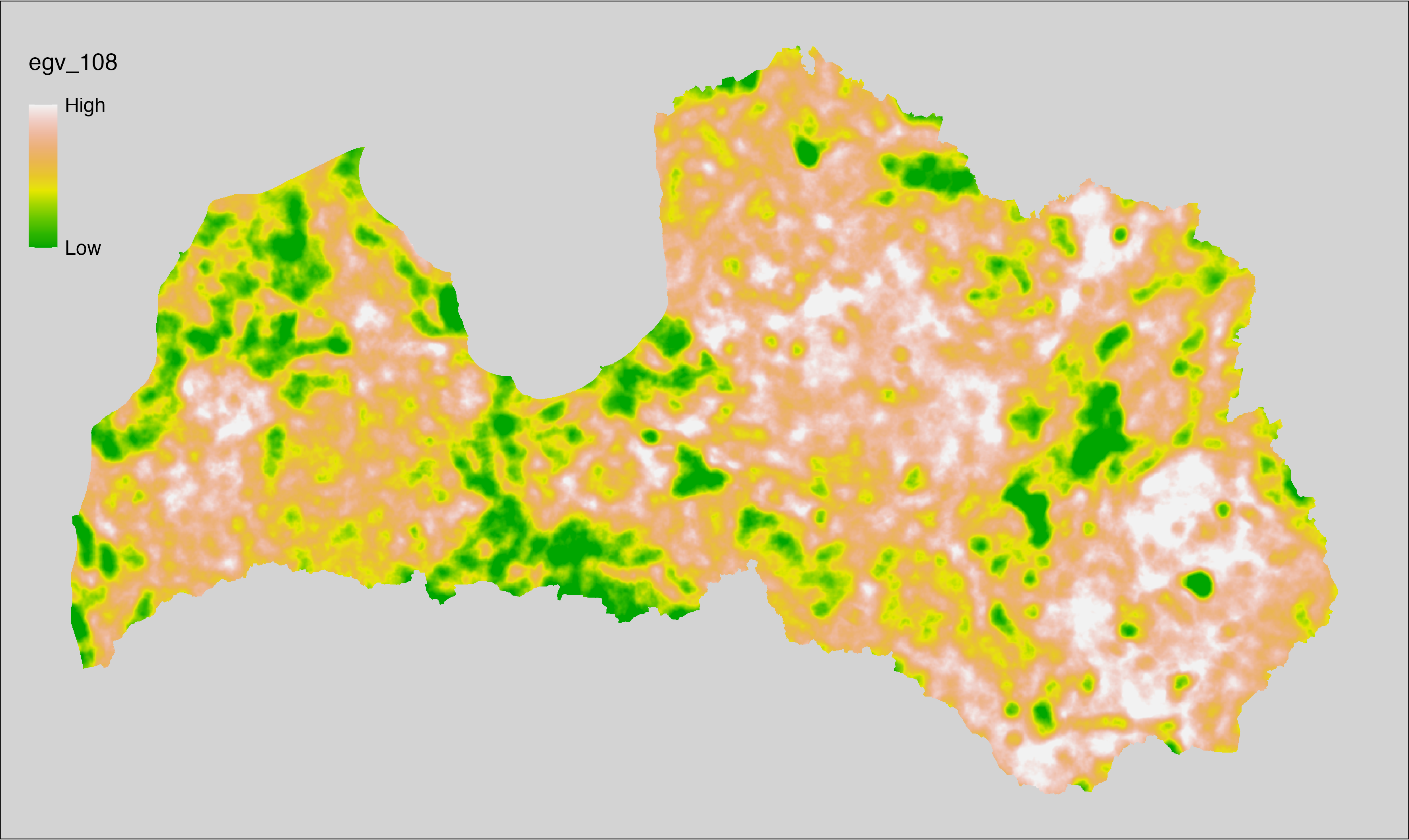
6.109 Diversity_Total_r10000
filename: Diversity_Total_r10000.tif
layername: egv_109
English name: Average combined landscape α-diversity of 500 m grid cells within the 10 km landscape
Latvian name: Vidējā visu ainavas klašu 500 m šūnu α-daudzveidība 10 km ainavā
Procedure: Derived from the Landscape diversity, more precisely
Overall landscape diversity. The average value of 25 ha cells diversity index
values is calculated using the workflow egvtools::radius_function(). To
prevent possible data loss at edge cells, inverse distance weighted
(power = 2) gap filling is implemented. File is written twice, to ensure
layername. Finally, the layer is standardised
by subtracting the arithmetic mean and dividing by the root mean squared error.
Code
# libs ----
if(!require(egvtools)) {remotes::install_github("aavotins/egvtools"); require(egvtools)}
if(!require(terra)) {install.packages("terra"); require(terra)}
# templates ----
template100=rast("./Templates/TemplateRasters/LV100m_10km.tif")
# radii
radius_function(
kvadrati_path = "./Templates/TemplateGrids/tiles/",
radii_path = "./Templates/TemplateGridPoints/tiles/",
tikls100_path = "./Templates/TemplateGrids/tikls100_sauzeme.parquet",
template_path = "./Templates/TemplateRasters/LV100m_10km.tif",
input_layers = c("./RasterGrids_500m/2024/Diversity_GeneralLandscape_500x.tif"),
layer_prefixes = c("Diversity_Total"),
output_dir = "./RasterGrids_100m/2024/RAW/",
n_workers = 12,
radii = c("r10000"),
radius_mode = "sparse",
extract_fun = "mean",
fill_missing = TRUE,
IDW_weight = 2,
future_max_size = 5 * 1024^3)
# Diversity_Total_r10000.tif egv_109
slanis=rast("./RasterGrids_100m/2024/RAW/Diversity_Total_r10000.tif")
names(slanis)="egv_109"
slanis2=project(slanis,template100)
writeRaster(slanis2,
"./RasterGrids_100m/2024/RAW/Diversity_Total_r10000.tif",
overwrite=TRUE)
# standardisation ----
if(!require(terra)) {install.packages("terra"); require(terra)}
if(!require(tidyverse)) {install.packages("tidyverse"); require(tidyverse)}
nosaukums="Diversity_Total_r10000.tif"
ielasisanas_cels=paste0("./RasterGrids_100m/2024/RAW/",nosaukums)
saglabasanas_cels=paste0("./RasterGrids_100m/2024/Scaled/",nosaukums)
slanis=rast(ielasisanas_cels)
videjais=global(slanis,fun="mean",na.rm=TRUE)
centrets=slanis-videjais[,1]
standartnovirze=terra::global(centrets,fun="rms",na.rm=TRUE)
merogots=centrets/standartnovirze[,1]
writeRaster(merogots,
filename=saglabasanas_cels,
overwrite=TRUE)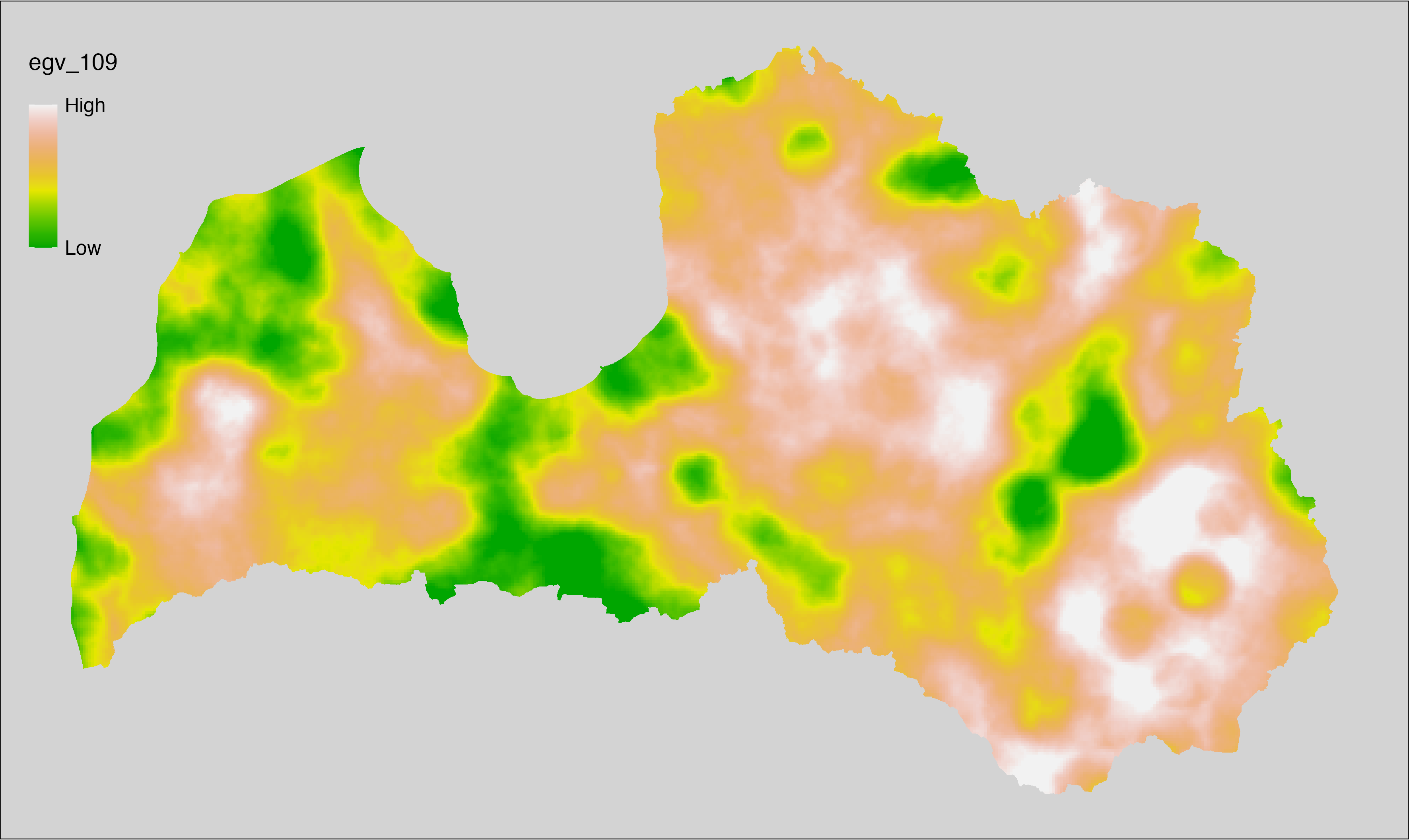
6.110 Edges_Bogs-Trees_cell
filename: Edges_Bogs-Trees_cell.tif
layername: egv_110
English name: Edge pixels of Bogs, Mires bordering with Trees within the analysis cell (1 ha)
Latvian name: Purvu malu ar kokiem pikseļu skaits analīzes šūnā (1 ha)
Procedure: First, values from 620 to 700 from the Landscape
classification are coded as 0, and all other values as NA. Then bog and
transitional mire layers from the EDI are reclassified to presence-only
(value 1) and combined. Then, bog-and-mire layer (1 = presence) is covered over
tree layer (presence = 0) and written to file (matching the input). Then, with
the workflow egvtools::landscape_function() total edge between the two classes
is calculated. During the calculation of the landscape metric, inverse distance weighted
(power = 2) gap filling on the output is applied to ensure no missing values
at the edges. Finally, the layer is standardised by subtracting the arithmetic
mean and dividing by the root mean squared error.
Code
# libs ----
if(!require(terra)) {install.packages("terra"); require(terra)}
if(!require(egvtools)) {remotes::install_github("aavotins/egvtools"); require(egvtools)}
if(!require(sf)) {install.packages("sf"); require(sf)}
if(!require(sfarrow)) {install.packages("sfarrow"); require(sfarrow)}
if(!require(raster)) {install.packages("raster"); require(raster)}
if(!require(fasterize)) {install.packages("fasterize"); require(fasterize)}
if(!require(tidyverse)) {install.packages("tidyverse"); require(tidyverse)}
# Templates -----
template10=rast("./Templates/TemplateRasters/LV10m_10km.tif")
nulls10=rast("./Templates/TemplateRasters/nulls_LV10m_10km.tif")
# simple landscape ----
simple_landscape=rast("./RasterGrids_10m/2024/Ainava_vienk_mask.tif")
# Edges_Bogs-Trees_input.tif ----
trees_from620=ifel(simple_landscape>=620 & simple_landscape<700,0,NA)
plot(trees_from620)
bogs=rast("./RasterGrids_10m/2024/EDI_BogsYN.tif")
bogs=subst(bogs,0,NA)
plot(bogs)
mires=rast("./RasterGrids_10m/2024/EDI_TransitionalMiresYN.tif")
mires=subst(mires,0,NA)
plot(mires)
bogs_mires=cover(bogs,mires)
plot(bogs_mires)
bm_trees=cover(bogs_mires,trees_from620)
plot(bm_trees)
edge_bm_trees=project(bm_trees,template10,
filename="./RasterGrids_10m/2024/Edges_Bogs-Trees_input.tif",
overwrite=TRUE)
rm(edge_bm_trees)
rm(bm_trees)
# Edges_Bogs-Trees_cell.tif egv_110
landscape_function(
landscape = "./RasterGrids_10m/2024/Edges_Bogs-Trees_input.tif",
zones = "./Templates/TemplateGrids/tikls100_sauzeme.parquet",
id_field = "id",
tile_field = "tks50km",
template = "./Templates/TemplateRasters/LV100m_10km.tif",
out_dir = "./RasterGrids_100m/2024/RAW",
out_filename = "Edges_Bogs-Trees_cell.tif",
out_layername = "egv_110",
what = "lsm_l_te",
lm_args = list(count_boundary = FALSE),
rasterize_engine = "fasterize",
n_workers = 12,
future_max_size = 20 * 1024^3,
fill_gaps = TRUE,
plot_gaps = FALSE,
plot_result = FALSE
)
# standardisation ----
if(!require(terra)) {install.packages("terra"); require(terra)}
if(!require(tidyverse)) {install.packages("tidyverse"); require(tidyverse)}
nosaukums="Edges_Bogs-Trees_cell.tif"
ielasisanas_cels=paste0("./RasterGrids_100m/2024/RAW/",nosaukums)
saglabasanas_cels=paste0("./RasterGrids_100m/2024/Scaled/",nosaukums)
slanis=rast(ielasisanas_cels)
videjais=global(slanis,fun="mean",na.rm=TRUE)
centrets=slanis-videjais[,1]
standartnovirze=terra::global(centrets,fun="rms",na.rm=TRUE)
merogots=centrets/standartnovirze[,1]
writeRaster(merogots,
filename=saglabasanas_cels,
overwrite=TRUE)
6.111 Edges_Bogs-Trees_r500
filename: Edges_Bogs-Trees_r500.tif
layername: egv_111
English name: Edge pixels of Bogs, Mires bordering with Trees within the 0.5 km landscape
Latvian name: Purvu malu ar kokiem pikseļu skaits 0,5 km ainavā
Procedure: The total edge within a 500 m radius around the analysis grid cell is
calculated as the area-weighted sum of the analysis cells inside the
buffer, using the workflow egvtools::radius_function(). During the calculation of the landscape metric,
inverse distance weighted (power = 2) gap filling on the output is applied
to ensure no missing values at the edges. Then the layer is rewritten to set
its name. Finally, the layer is standardised by subtracting the arithmetic
mean and dividing by the root mean squared error.
Code
# libs ----
if(!require(terra)) {install.packages("terra"); require(terra)}
if(!require(egvtools)) {remotes::install_github("aavotins/egvtools"); require(egvtools)}
# Templates -----
template100=rast("./Templates/TemplateRasters/LV100m_10km.tif")
# radii
radius_function(
kvadrati_path = "./Templates/TemplateGrids/tiles/",
radii_path = "./Templates/TemplateGridPoints/tiles/",
tikls100_path = "./Templates/TemplateGrids/tikls100_sauzeme.parquet",
template_path = "./Templates/TemplateRasters/LV100m_10km.tif",
input_layers = c("./RasterGrids_100m/2024/RAW/Edges_Bogs-Trees_cell.tif"),
layer_prefixes = c("Edges_Bogs-Trees"),
output_dir = "./RasterGrids_100m/2024/RAW/",
n_workers = 4,
radii = c("r500"),
radius_mode = "sparse",
extract_fun = "sum",
fill_missing = TRUE,
IDW_weight = 2,
future_max_size = 20 * 1024^3)
# Edges_Bogs-Trees_r500.tif egv_111
slanis=rast("./RasterGrids_100m/2024/RAW/Edges_Bogs-Trees_r500.tif")
names(slanis)="egv_111"
slanis2=project(slanis,template100)
writeRaster(slanis2,
"./RasterGrids_100m/2024/RAW/Edges_Bogs-Trees_r500.tif",
overwrite=TRUE)
# standardisation ----
if(!require(terra)) {install.packages("terra"); require(terra)}
if(!require(tidyverse)) {install.packages("tidyverse"); require(tidyverse)}
nosaukums="Edges_Bogs-Trees_r500.tif"
ielasisanas_cels=paste0("./RasterGrids_100m/2024/RAW/",nosaukums)
saglabasanas_cels=paste0("./RasterGrids_100m/2024/Scaled/",nosaukums)
slanis=rast(ielasisanas_cels)
videjais=global(slanis,fun="mean",na.rm=TRUE)
centrets=slanis-videjais[,1]
standartnovirze=terra::global(centrets,fun="rms",na.rm=TRUE)
merogots=centrets/standartnovirze[,1]
writeRaster(merogots,
filename=saglabasanas_cels,
overwrite=TRUE)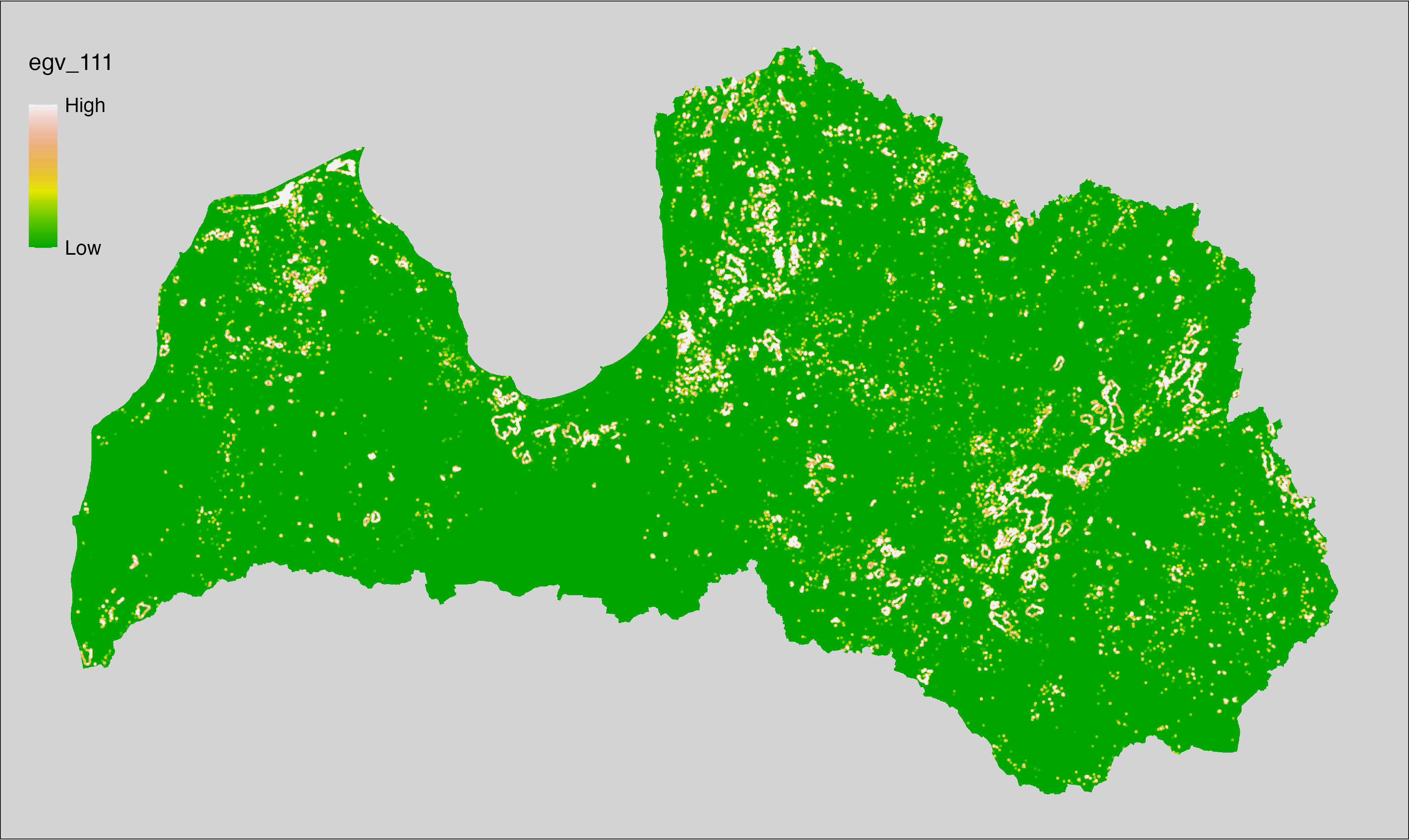
6.112 Edges_Bogs-Trees_r1250
filename: Edges_Bogs-Trees_r1250.tif
layername: egv_112
English name: Edge pixels of Bogs, Mires bordering with Trees within the 1.25 km landscape
Latvian name: Purvu malu ar kokiem pikseļu skaits 1,25 km ainavā
Procedure: The total edge within a 1250 m radius around the analysis grid cell is
calculated as the area-weighted sum of the analysis cells inside the
buffer, using the workflow egvtools::radius_function(). During the calculation of the landscape metric,
inverse distance weighted (power = 2) gap filling on the output is applied
to ensure no missing values at the edges. Then the layer is rewritten to set
its name. Finally, the layer is standardised by subtracting the arithmetic
mean and dividing by the root mean squared error.
Code
# libs ----
if(!require(terra)) {install.packages("terra"); require(terra)}
if(!require(egvtools)) {remotes::install_github("aavotins/egvtools"); require(egvtools)}
# Templates -----
template100=rast("./Templates/TemplateRasters/LV100m_10km.tif")
# radii
radius_function(
kvadrati_path = "./Templates/TemplateGrids/tiles/",
radii_path = "./Templates/TemplateGridPoints/tiles/",
tikls100_path = "./Templates/TemplateGrids/tikls100_sauzeme.parquet",
template_path = "./Templates/TemplateRasters/LV100m_10km.tif",
input_layers = c("./RasterGrids_100m/2024/RAW/Edges_Bogs-Trees_cell.tif"),
layer_prefixes = c("Edges_Bogs-Trees"),
output_dir = "./RasterGrids_100m/2024/RAW/",
n_workers = 4,
radii = c("r1250"),
radius_mode = "sparse",
extract_fun = "sum",
fill_missing = TRUE,
IDW_weight = 2,
future_max_size = 20 * 1024^3)
# Edges_Bogs-Trees_r1250.tif egv_112
slanis=rast("./RasterGrids_100m/2024/RAW/Edges_Bogs-Trees_r1250.tif")
names(slanis)="egv_112"
slanis2=project(slanis,template100)
writeRaster(slanis2,
"./RasterGrids_100m/2024/RAW/Edges_Bogs-Trees_r1250.tif",
overwrite=TRUE)
# standardisation ----
if(!require(terra)) {install.packages("terra"); require(terra)}
if(!require(tidyverse)) {install.packages("tidyverse"); require(tidyverse)}
nosaukums="Edges_Bogs-Trees_r1250.tif"
ielasisanas_cels=paste0("./RasterGrids_100m/2024/RAW/",nosaukums)
saglabasanas_cels=paste0("./RasterGrids_100m/2024/Scaled/",nosaukums)
slanis=rast(ielasisanas_cels)
videjais=global(slanis,fun="mean",na.rm=TRUE)
centrets=slanis-videjais[,1]
standartnovirze=terra::global(centrets,fun="rms",na.rm=TRUE)
merogots=centrets/standartnovirze[,1]
writeRaster(merogots,
filename=saglabasanas_cels,
overwrite=TRUE)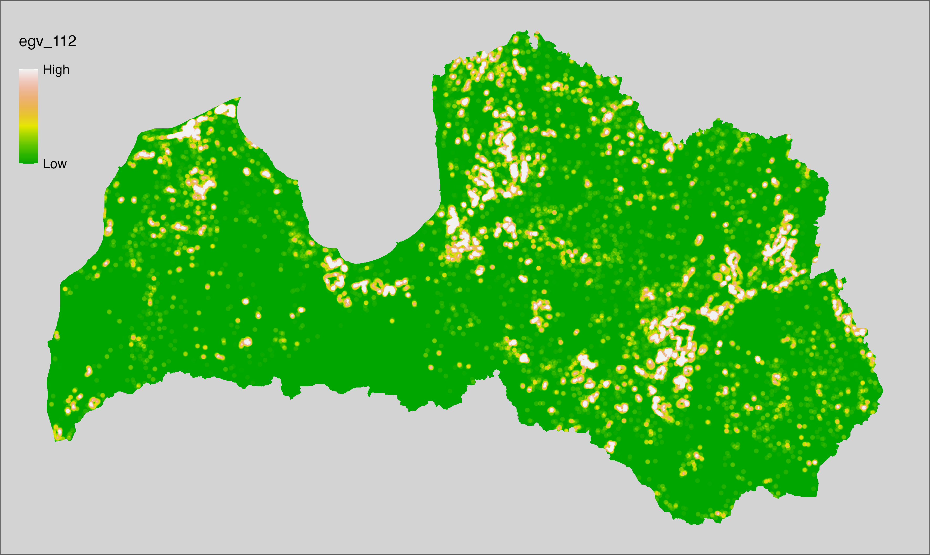
6.113 Edges_Bogs-Trees_r3000
filename: Edges_Bogs-Trees_r3000.tif
layername: egv_113
English name: Edge pixels of Bogs, Mires bordering with Trees within the 3 km landscape
Latvian name: Purvu malu ar kokiem pikseļu skaits 3 km ainavā
Procedure: Total edge within a 3000 m radius around the analysis grid cell is
calculated as the area-weighted sum of the analysis cells inside the
buffer, using the workflow egvtools::radius_function(). During the calculation of the landscape metric,
inverse distance weighted (power = 2) gap filling on the output is applied
to ensure no missing values at the edges. Then the layer is rewritten to set
its name. Finally, the layer is standardised by subtracting the arithmetic
mean and dividing by the root mean squared error.
Code
# libs ----
if(!require(terra)) {install.packages("terra"); require(terra)}
if(!require(egvtools)) {remotes::install_github("aavotins/egvtools"); require(egvtools)}
# Templates -----
template100=rast("./Templates/TemplateRasters/LV100m_10km.tif")
# radii
radius_function(
kvadrati_path = "./Templates/TemplateGrids/tiles/",
radii_path = "./Templates/TemplateGridPoints/tiles/",
tikls100_path = "./Templates/TemplateGrids/tikls100_sauzeme.parquet",
template_path = "./Templates/TemplateRasters/LV100m_10km.tif",
input_layers = c("./RasterGrids_100m/2024/RAW/Edges_Bogs-Trees_cell.tif"),
layer_prefixes = c("Edges_Bogs-Trees"),
output_dir = "./RasterGrids_100m/2024/RAW/",
n_workers = 4,
radii = c("r3000"),
radius_mode = "sparse",
extract_fun = "sum",
fill_missing = TRUE,
IDW_weight = 2,
future_max_size = 20 * 1024^3)
# Edges_Bogs-Trees_r3000.tif egv_113
slanis=rast("./RasterGrids_100m/2024/RAW/Edges_Bogs-Trees_r3000.tif")
names(slanis)="egv_113"
slanis2=project(slanis,template100)
writeRaster(slanis2,
"./RasterGrids_100m/2024/RAW/Edges_Bogs-Trees_r3000.tif",
overwrite=TRUE)
# standardisation ----
if(!require(terra)) {install.packages("terra"); require(terra)}
if(!require(tidyverse)) {install.packages("tidyverse"); require(tidyverse)}
nosaukums="Edges_Bogs-Trees_r3000.tif"
ielasisanas_cels=paste0("./RasterGrids_100m/2024/RAW/",nosaukums)
saglabasanas_cels=paste0("./RasterGrids_100m/2024/Scaled/",nosaukums)
slanis=rast(ielasisanas_cels)
videjais=global(slanis,fun="mean",na.rm=TRUE)
centrets=slanis-videjais[,1]
standartnovirze=terra::global(centrets,fun="rms",na.rm=TRUE)
merogots=centrets/standartnovirze[,1]
writeRaster(merogots,
filename=saglabasanas_cels,
overwrite=TRUE)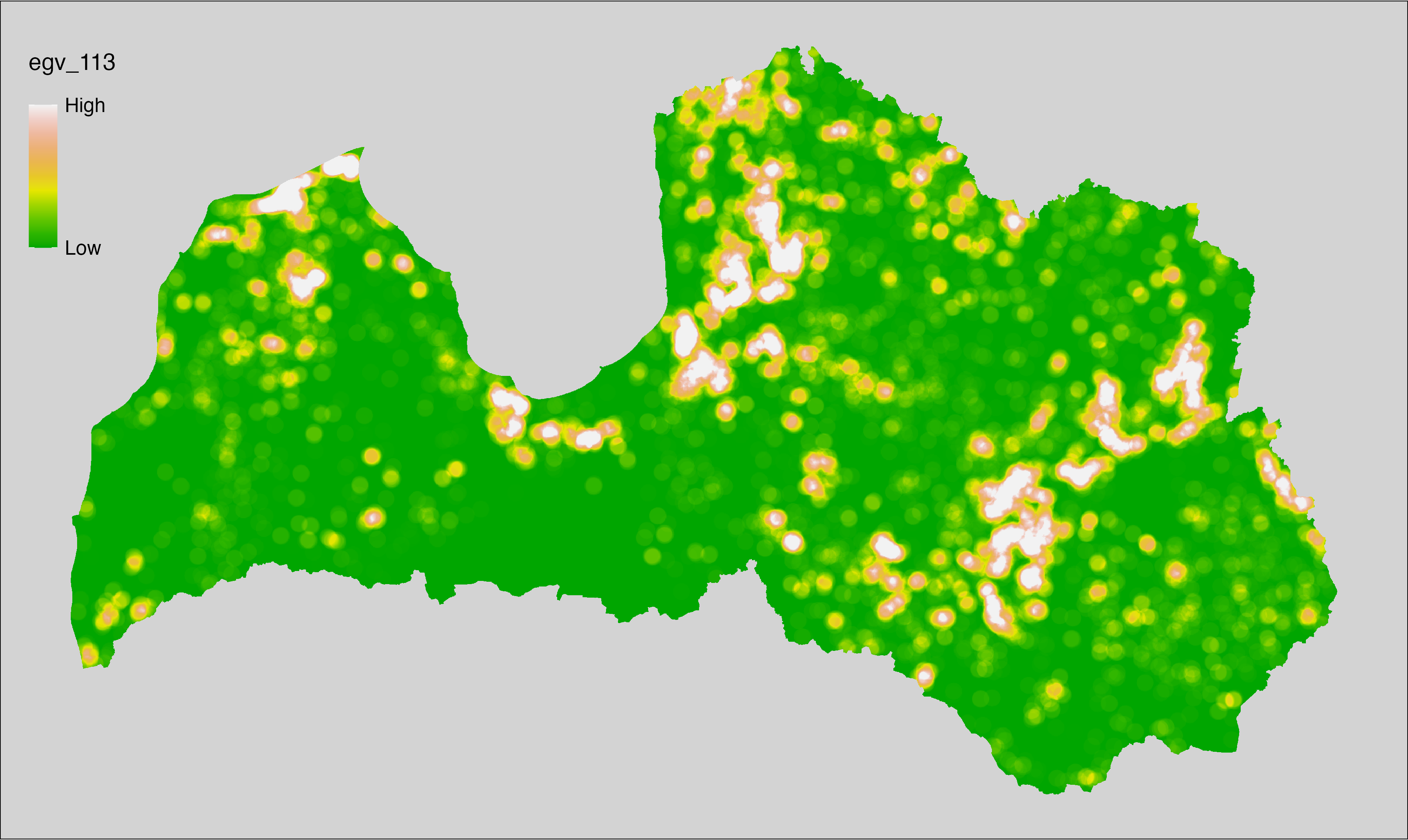
6.114 Edges_Bogs-Trees_r10000
filename: Edges_Bogs-Trees_r10000.tif
layername: egv_114
English name: Edge pixels of Bogs, Mires bordering with Trees within the 10 km landscape
Latvian name: Purvu malu ar kokiem pikseļu skaits 10 km ainavā
Procedure: The total edge within a 10000 m radius around the analysis grid cell is
calculated as the area-weighted sum of the analysis cells inside the
buffer, using the workflow egvtools::radius_function(). During the calculation of the landscape metric,
inverse distance weighted (power = 2) gap filling on the output is applied
to ensure no missing values at the edges. Then the layer is rewritten to set
its name. Finally, the layer is standardised by subtracting the arithmetic
mean and dividing by the root mean squared error.
Code
# libs ----
if(!require(terra)) {install.packages("terra"); require(terra)}
if(!require(egvtools)) {remotes::install_github("aavotins/egvtools"); require(egvtools)}
# Templates -----
template100=rast("./Templates/TemplateRasters/LV100m_10km.tif")
# radii
radius_function(
kvadrati_path = "./Templates/TemplateGrids/tiles/",
radii_path = "./Templates/TemplateGridPoints/tiles/",
tikls100_path = "./Templates/TemplateGrids/tikls100_sauzeme.parquet",
template_path = "./Templates/TemplateRasters/LV100m_10km.tif",
input_layers = c("./RasterGrids_100m/2024/RAW/Edges_Bogs-Trees_cell.tif"),
layer_prefixes = c("Edges_Bogs-Trees"),
output_dir = "./RasterGrids_100m/2024/RAW/",
n_workers = 4,
radii = c("r10000"),
radius_mode = "sparse",
extract_fun = "sum",
fill_missing = TRUE,
IDW_weight = 2,
future_max_size = 20 * 1024^3)
# Edges_Bogs-Trees_r10000.tif egv_114
slanis=rast("./RasterGrids_100m/2024/RAW/Edges_Bogs-Trees_r10000.tif")
names(slanis)="egv_114"
slanis2=project(slanis,template100)
writeRaster(slanis2,
"./RasterGrids_100m/2024/RAW/Edges_Bogs-Trees_r10000.tif",
overwrite=TRUE)
# standardisation ----
if(!require(terra)) {install.packages("terra"); require(terra)}
if(!require(tidyverse)) {install.packages("tidyverse"); require(tidyverse)}
nosaukums="Edges_Bogs-Trees_r10000.tif"
ielasisanas_cels=paste0("./RasterGrids_100m/2024/RAW/",nosaukums)
saglabasanas_cels=paste0("./RasterGrids_100m/2024/Scaled/",nosaukums)
slanis=rast(ielasisanas_cels)
videjais=global(slanis,fun="mean",na.rm=TRUE)
centrets=slanis-videjais[,1]
standartnovirze=terra::global(centrets,fun="rms",na.rm=TRUE)
merogots=centrets/standartnovirze[,1]
writeRaster(merogots,
filename=saglabasanas_cels,
overwrite=TRUE)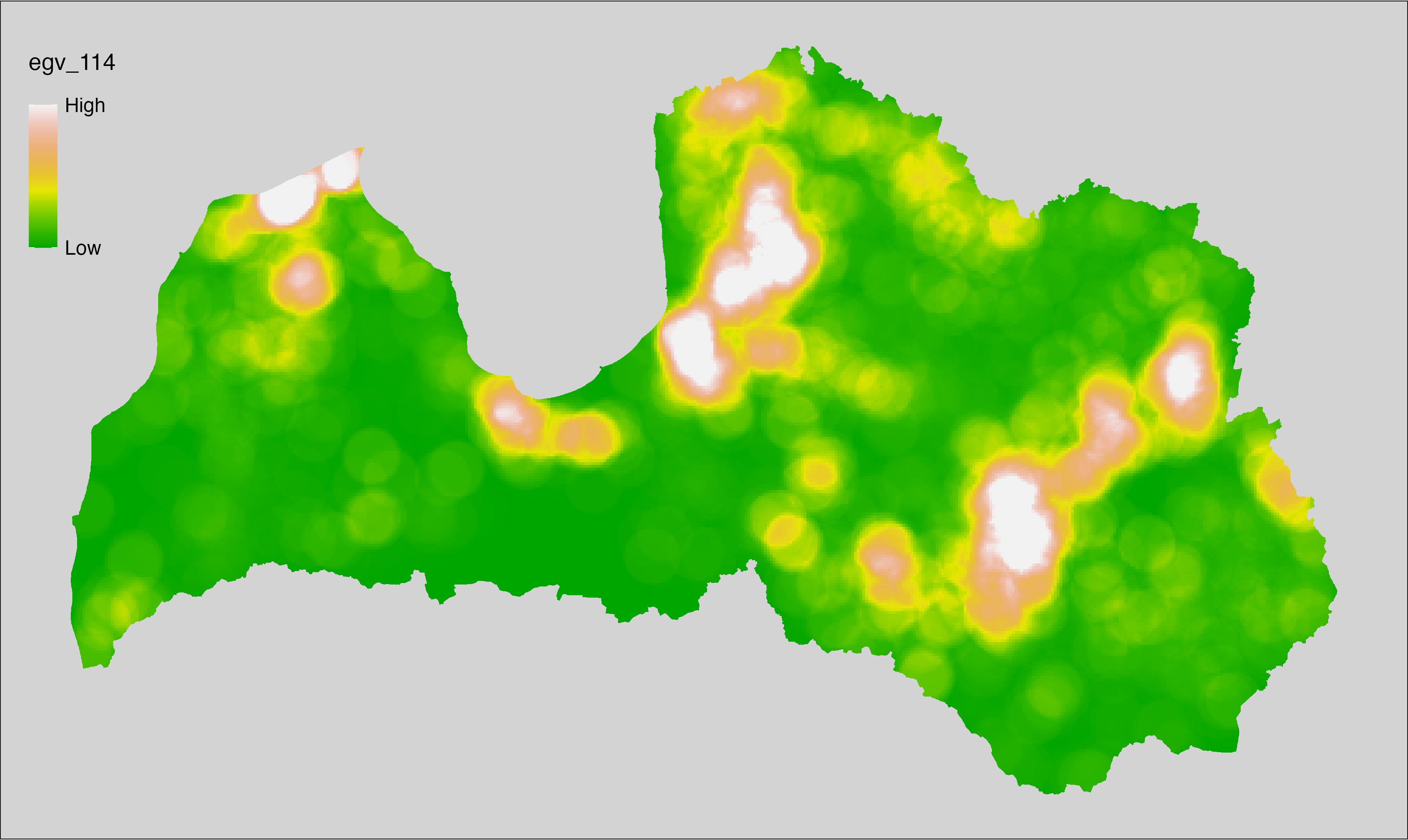
6.115 Edges_Bogs-Water_cell
filename: Edges_Bogs-Water_cell.tif
layername: egv_115
English name: Edge pixels of Bogs, Mires bordering with Water within the analysis cell (1 ha)
Latvian name: Purvu malu ar ūdeni pikseļu skaits analīzes šūnā (1 ha)
Procedure: First, values 200 from the Landscape classification are
coded as 0, and all other values as NA. Then bog and transitional mire layers from
EDI are reclassified to presence-only (value 1) and combined. Then,
bog-and-mire layer (1 = presence) is covered over water layer (presence = 0) and
written to file (matching the input). Then, using the workflow
egvtools::landscape_function() total edge between the two classes is
calculated. During the calculation of the landscape metric, inverse distance weighted
(power = 2) gap filling on the output is applied to ensure no missing values
at the edges. Finally, the layer is standardised by subtracting the arithmetic
mean and dividing by the root mean squared error.
Code
# libs ----
if(!require(terra)) {install.packages("terra"); require(terra)}
if(!require(egvtools)) {remotes::install_github("aavotins/egvtools"); require(egvtools)}
if(!require(sf)) {install.packages("sf"); require(sf)}
if(!require(sfarrow)) {install.packages("sfarrow"); require(sfarrow)}
if(!require(raster)) {install.packages("raster"); require(raster)}
if(!require(fasterize)) {install.packages("fasterize"); require(fasterize)}
if(!require(tidyverse)) {install.packages("tidyverse"); require(tidyverse)}
# Templates -----
template10=rast("./Templates/TemplateRasters/LV10m_10km.tif")
nulls10=rast("./Templates/TemplateRasters/nulls_LV10m_10km.tif")
# simple landscape ----
simple_landscape=rast("./RasterGrids_10m/2024/Ainava_vienk_mask.tif")
# Edges_Bogs-Water_input.tif ----
bogs=rast("./RasterGrids_10m/2024/EDI_BogsYN.tif")
bogs=subst(bogs,0,NA)
plot(bogs)
mires=rast("./RasterGrids_10m/2024/EDI_TransitionalMiresYN.tif")
mires=subst(mires,0,NA)
plot(mires)
bogs_mires=cover(bogs,mires)
plot(bogs_mires)
water=ifel(simple_landscape==200,0,NA)
plot(water)
bm_water=cover(bogs_mires,water)
plot(bm_water)
edge_bm_water=project(bm_water,template10,
filename="./RasterGrids_10m/2024/Edges_Bogs-Water_input.tif",
overwrite=TRUE)
rm(edge_bm_water)
rm(bm_water)
# Edges_Bogs-Water_cell.tif egv_115 ----
landscape_function(
landscape = "./RasterGrids_10m/2024/Edges_Bogs-Water_input.tif",
zones = "./Templates/TemplateGrids/tikls100_sauzeme.parquet",
id_field = "id",
tile_field = "tks50km",
template = "./Templates/TemplateRasters/LV100m_10km.tif",
out_dir = "./RasterGrids_100m/2024/RAW",
out_filename = "Edges_Bogs-Water_cell.tif",
out_layername = "egv_115",
what = "lsm_l_te",
lm_args = list(count_boundary = FALSE),
rasterize_engine = "fasterize",
n_workers = 12,
future_max_size = 20 * 1024^3,
fill_gaps = TRUE,
plot_gaps = FALSE,
plot_result = FALSE
)
# standardisation ----
if(!require(terra)) {install.packages("terra"); require(terra)}
if(!require(tidyverse)) {install.packages("tidyverse"); require(tidyverse)}
nosaukums="Edges_Bogs-Water_cell.tif"
ielasisanas_cels=paste0("./RasterGrids_100m/2024/RAW/",nosaukums)
saglabasanas_cels=paste0("./RasterGrids_100m/2024/Scaled/",nosaukums)
slanis=rast(ielasisanas_cels)
videjais=global(slanis,fun="mean",na.rm=TRUE)
centrets=slanis-videjais[,1]
standartnovirze=terra::global(centrets,fun="rms",na.rm=TRUE)
merogots=centrets/standartnovirze[,1]
writeRaster(merogots,
filename=saglabasanas_cels,
overwrite=TRUE)
6.116 Edges_Bogs-Water_r500
filename: Edges_Bogs-Water_r500.tif
layername: egv_116
English name: Edge pixels of Bogs, Mires bordering with Water within the 0.5 km landscape
Latvian name: Purvu malu ar ūdeni pikseļu skaits 0,5 km ainavā
Procedure: The total edge within a 500 m radius around the analysis grid cell is
calculated as the area-weighted sum of the analysis cells inside the
buffer, using the workflow egvtools::radius_function(). During the calculation of the landscape metric,
inverse distance weighted (power = 2) gap filling on the output is applied
to ensure no missing values at the edges. Then the layer is rewritten to set
its name. Finally, the layer is standardised by subtracting the arithmetic
mean and dividing by the root mean squared error.
Code
# libs ----
if(!require(terra)) {install.packages("terra"); require(terra)}
if(!require(egvtools)) {remotes::install_github("aavotins/egvtools"); require(egvtools)}
# Templates -----
template100=rast("./Templates/TemplateRasters/LV100m_10km.tif")
# radii ----
radius_function(
kvadrati_path = "./Templates/TemplateGrids/tiles/",
radii_path = "./Templates/TemplateGridPoints/tiles/",
tikls100_path = "./Templates/TemplateGrids/tikls100_sauzeme.parquet",
template_path = "./Templates/TemplateRasters/LV100m_10km.tif",
input_layers = c("./RasterGrids_100m/2024/RAW/Edges_Bogs-Water_cell.tif"),
layer_prefixes = c("Edges_Bogs-Water"),
output_dir = "./RasterGrids_100m/2024/RAW/",
n_workers = 12,
radii = c("r500"),
radius_mode = "sparse",
extract_fun = "sum",
fill_missing = TRUE,
IDW_weight = 2,
future_max_size = 20 * 1024^3)
# Edges_Bogs-Water_r500.tif egv_116
slanis=rast("./RasterGrids_100m/2024/RAW/Edges_Bogs-Water_r500.tif")
names(slanis)="egv_116"
slanis2=project(slanis,template100)
writeRaster(slanis2,
"./RasterGrids_100m/2024/RAW/Edges_Bogs-Water_r500.tif",
overwrite=TRUE)
# standardisation ----
if(!require(terra)) {install.packages("terra"); require(terra)}
if(!require(tidyverse)) {install.packages("tidyverse"); require(tidyverse)}
nosaukums="Edges_Bogs-Water_r500.tif"
ielasisanas_cels=paste0("./RasterGrids_100m/2024/RAW/",nosaukums)
saglabasanas_cels=paste0("./RasterGrids_100m/2024/Scaled/",nosaukums)
slanis=rast(ielasisanas_cels)
videjais=global(slanis,fun="mean",na.rm=TRUE)
centrets=slanis-videjais[,1]
standartnovirze=terra::global(centrets,fun="rms",na.rm=TRUE)
merogots=centrets/standartnovirze[,1]
writeRaster(merogots,
filename=saglabasanas_cels,
overwrite=TRUE)
6.117 Edges_Bogs-Water_r1250
filename: Edges_Bogs-Water_r1250.tif
layername: egv_117
English name: Edge pixels of Bogs, Mires bordering with Water within the 1.25 km landscape
Latvian name: Purvu malu ar ūdeni pikseļu skaits 1,25 km ainavā
Procedure: The total edge within a 1250 m radius around the analysis grid cell is
calculated as the area-weighted sum of the analysis cells inside the
buffer, using the workflow egvtools::radius_function(). During the calculation of the landscape metric,
inverse distance weighted (power = 2) gap filling on the output is applied
to ensure no missing values at the edges. Then the layer is rewritten to set
its name. Finally, the layer is standardised by subtracting the arithmetic
mean and dividing by the root mean squared error.
Code
# libs ----
if(!require(terra)) {install.packages("terra"); require(terra)}
if(!require(egvtools)) {remotes::install_github("aavotins/egvtools"); require(egvtools)}
# Templates -----
template100=rast("./Templates/TemplateRasters/LV100m_10km.tif")
# radii ----
radius_function(
kvadrati_path = "./Templates/TemplateGrids/tiles/",
radii_path = "./Templates/TemplateGridPoints/tiles/",
tikls100_path = "./Templates/TemplateGrids/tikls100_sauzeme.parquet",
template_path = "./Templates/TemplateRasters/LV100m_10km.tif",
input_layers = c("./RasterGrids_100m/2024/RAW/Edges_Bogs-Water_cell.tif"),
layer_prefixes = c("Edges_Bogs-Water"),
output_dir = "./RasterGrids_100m/2024/RAW/",
n_workers = 12,
radii = c("r1250"),
radius_mode = "sparse",
extract_fun = "sum",
fill_missing = TRUE,
IDW_weight = 2,
future_max_size = 20 * 1024^3)
# Edges_Bogs-Water_r1250.tif egv_117
slanis=rast("./RasterGrids_100m/2024/RAW/Edges_Bogs-Water_r1250.tif")
names(slanis)="egv_117"
slanis2=project(slanis,template100)
writeRaster(slanis2,
"./RasterGrids_100m/2024/RAW/Edges_Bogs-Water_r1250.tif",
overwrite=TRUE)
# standardisation ----
if(!require(terra)) {install.packages("terra"); require(terra)}
if(!require(tidyverse)) {install.packages("tidyverse"); require(tidyverse)}
nosaukums="Edges_Bogs-Water_r1250.tif"
ielasisanas_cels=paste0("./RasterGrids_100m/2024/RAW/",nosaukums)
saglabasanas_cels=paste0("./RasterGrids_100m/2024/Scaled/",nosaukums)
slanis=rast(ielasisanas_cels)
videjais=global(slanis,fun="mean",na.rm=TRUE)
centrets=slanis-videjais[,1]
standartnovirze=terra::global(centrets,fun="rms",na.rm=TRUE)
merogots=centrets/standartnovirze[,1]
writeRaster(merogots,
filename=saglabasanas_cels,
overwrite=TRUE)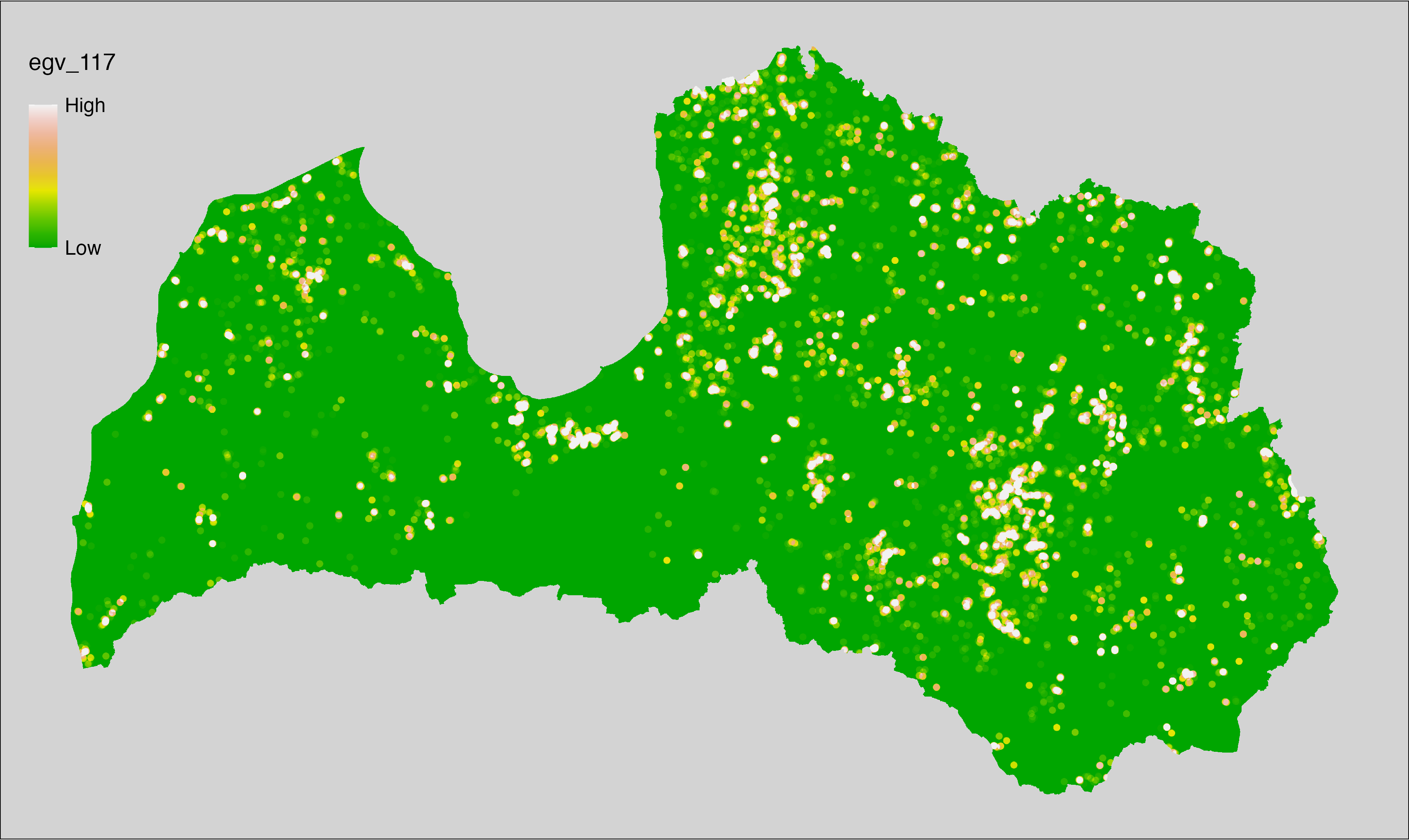
6.118 Edges_Bogs-Water_r3000
filename: Edges_Bogs-Water_r3000.tif
layername: egv_118
English name: Edge pixels of Bogs, Mires bordering with Water within the 3 km landscape
Latvian name: Purvu malu ar ūdeni pikseļu skaits 3 km ainavā
Procedure: The total edge within a 3000 m radius around the analysis grid cell is
calculated as the area-weighted sum of the analysis cells inside the
buffer, using the workflow egvtools::radius_function(). During the calculation of the landscape metric,
inverse distance weighted (power = 2) gap filling on the output is applied
to ensure no missing values at the edges. Then the layer is rewritten to set
its name. Finally, the layer is standardised by subtracting the arithmetic
mean and dividing by the root mean squared error.
Code
# libs ----
if(!require(terra)) {install.packages("terra"); require(terra)}
if(!require(egvtools)) {remotes::install_github("aavotins/egvtools"); require(egvtools)}
# Templates -----
template100=rast("./Templates/TemplateRasters/LV100m_10km.tif")
# radii ----
radius_function(
kvadrati_path = "./Templates/TemplateGrids/tiles/",
radii_path = "./Templates/TemplateGridPoints/tiles/",
tikls100_path = "./Templates/TemplateGrids/tikls100_sauzeme.parquet",
template_path = "./Templates/TemplateRasters/LV100m_10km.tif",
input_layers = c("./RasterGrids_100m/2024/RAW/Edges_Bogs-Water_cell.tif"),
layer_prefixes = c("Edges_Bogs-Water"),
output_dir = "./RasterGrids_100m/2024/RAW/",
n_workers = 12,
radii = c("r3000"),
radius_mode = "sparse",
extract_fun = "sum",
fill_missing = TRUE,
IDW_weight = 2,
future_max_size = 20 * 1024^3)
# Edges_Bogs-Water_r3000.tif egv_118
slanis=rast("./RasterGrids_100m/2024/RAW/Edges_Bogs-Water_r3000.tif")
names(slanis)="egv_118"
slanis2=project(slanis,template100)
writeRaster(slanis2,
"./RasterGrids_100m/2024/RAW/Edges_Bogs-Water_r3000.tif",
overwrite=TRUE)
# standardisation ----
if(!require(terra)) {install.packages("terra"); require(terra)}
if(!require(tidyverse)) {install.packages("tidyverse"); require(tidyverse)}
nosaukums="Edges_Bogs-Water_r3000.tif"
ielasisanas_cels=paste0("./RasterGrids_100m/2024/RAW/",nosaukums)
saglabasanas_cels=paste0("./RasterGrids_100m/2024/Scaled/",nosaukums)
slanis=rast(ielasisanas_cels)
videjais=global(slanis,fun="mean",na.rm=TRUE)
centrets=slanis-videjais[,1]
standartnovirze=terra::global(centrets,fun="rms",na.rm=TRUE)
merogots=centrets/standartnovirze[,1]
writeRaster(merogots,
filename=saglabasanas_cels,
overwrite=TRUE)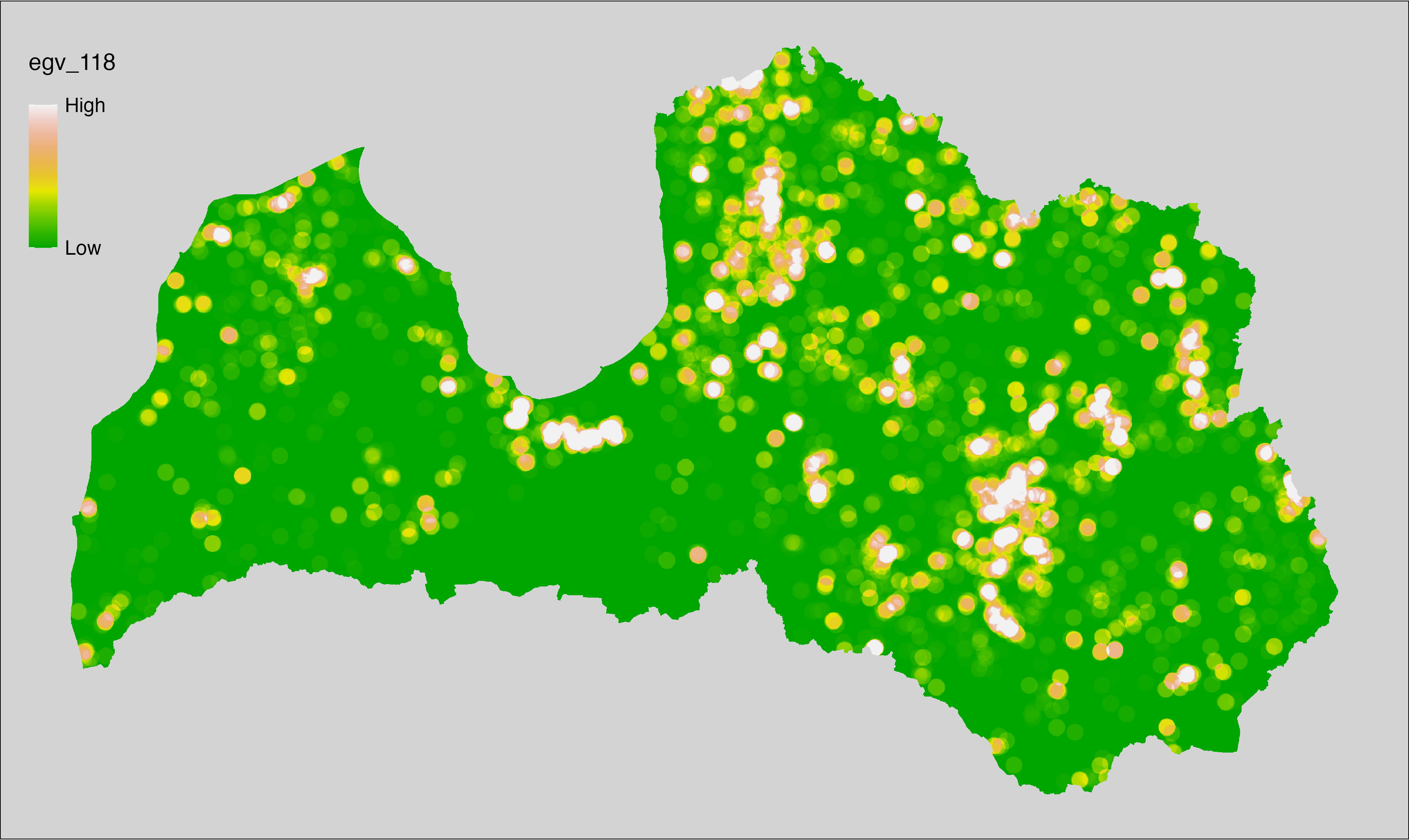
6.119 Edges_Bogs-Water_r10000
filename: Edges_Bogs-Water_r10000.tif
layername: egv_119
English name: Edge pixels of Bogs, Mires bordering with Water within the 10 km landscape
Latvian name: Purvu malu ar ūdeni pikseļu skaits 10 km ainavā
Procedure: The total edge within a 10000 m radius around the analysis grid cell is
calculated as the area-weighted sum of the analysis cells inside the
buffer, using the workflow egvtools::radius_function(). During the calculation of the landscape metric,
inverse distance weighted (power = 2) gap filling on the output is applied
to ensure no missing values at the edges. Then the layer is rewritten to set
its name. Finally, the layer is standardised by subtracting the arithmetic
mean and dividing by the root mean squared error.
Code
# libs ----
if(!require(terra)) {install.packages("terra"); require(terra)}
if(!require(egvtools)) {remotes::install_github("aavotins/egvtools"); require(egvtools)}
# Templates -----
template100=rast("./Templates/TemplateRasters/LV100m_10km.tif")
# radii ----
radius_function(
kvadrati_path = "./Templates/TemplateGrids/tiles/",
radii_path = "./Templates/TemplateGridPoints/tiles/",
tikls100_path = "./Templates/TemplateGrids/tikls100_sauzeme.parquet",
template_path = "./Templates/TemplateRasters/LV100m_10km.tif",
input_layers = c("./RasterGrids_100m/2024/RAW/Edges_Bogs-Water_cell.tif"),
layer_prefixes = c("Edges_Bogs-Water"),
output_dir = "./RasterGrids_100m/2024/RAW/",
n_workers = 12,
radii = c("r10000"),
radius_mode = "sparse",
extract_fun = "sum",
fill_missing = TRUE,
IDW_weight = 2,
future_max_size = 20 * 1024^3)
# Edges_Bogs-Water_r10000.tif egv_119
slanis=rast("./RasterGrids_100m/2024/RAW/Edges_Bogs-Water_r10000.tif")
names(slanis)="egv_119"
slanis2=project(slanis,template100)
writeRaster(slanis2,
"./RasterGrids_100m/2024/RAW/Edges_Bogs-Water_r10000.tif",
overwrite=TRUE)
# standardisation ----
if(!require(terra)) {install.packages("terra"); require(terra)}
if(!require(tidyverse)) {install.packages("tidyverse"); require(tidyverse)}
nosaukums="Edges_Bogs-Water_r10000.tif"
ielasisanas_cels=paste0("./RasterGrids_100m/2024/RAW/",nosaukums)
saglabasanas_cels=paste0("./RasterGrids_100m/2024/Scaled/",nosaukums)
slanis=rast(ielasisanas_cels)
videjais=global(slanis,fun="mean",na.rm=TRUE)
centrets=slanis-videjais[,1]
standartnovirze=terra::global(centrets,fun="rms",na.rm=TRUE)
merogots=centrets/standartnovirze[,1]
writeRaster(merogots,
filename=saglabasanas_cels,
overwrite=TRUE)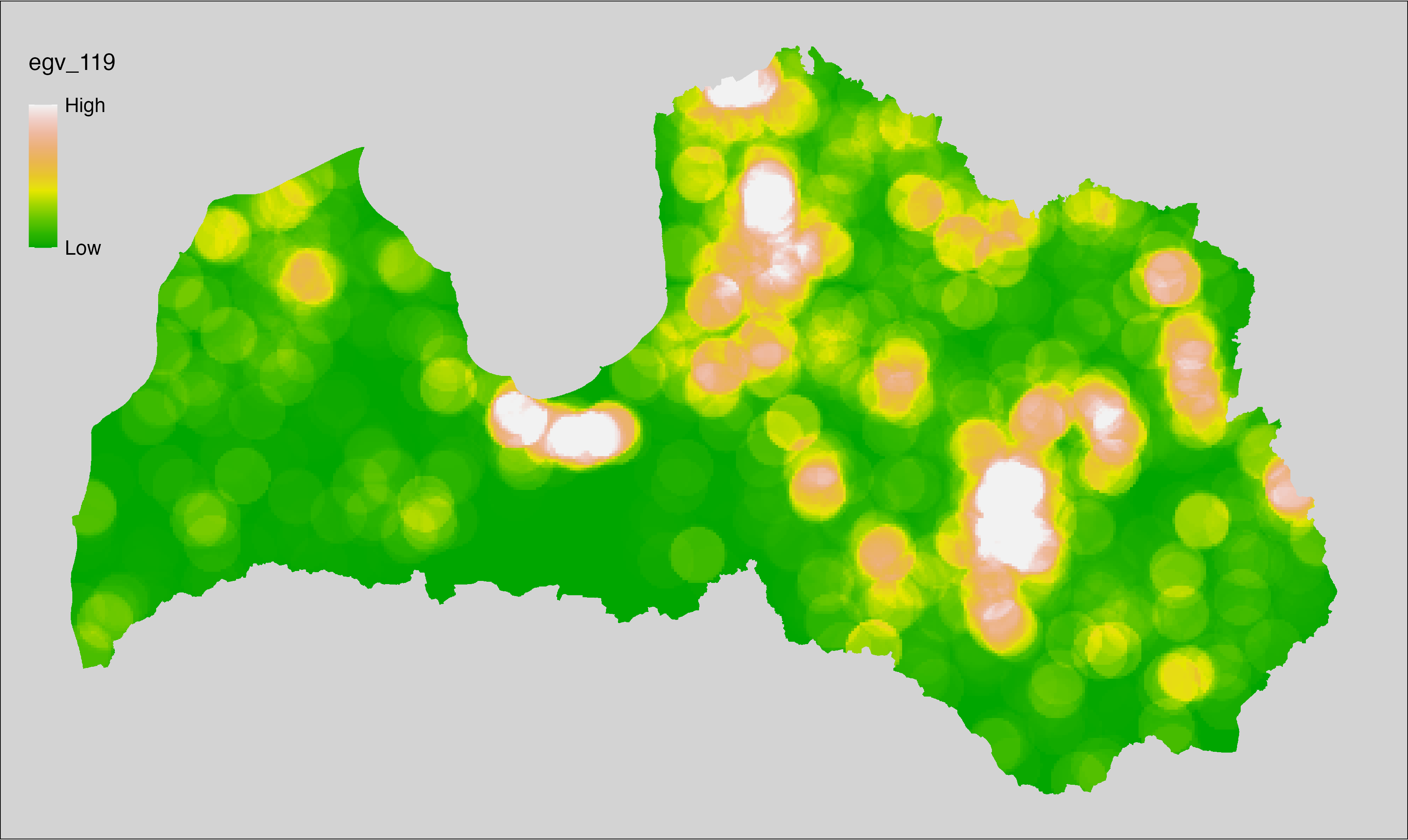
6.120 Edges_Farmland-Builtup_cell
filename: Edges_Farmland-Builtup_cell.tif
layername: egv_120
English name: Edge pixels of Farmland bordering with Built-Up areas within the analysis cell (1 ha)
Latvian name: Lauksaimniecības zemju malu ar apbūvi pikseļu skaits analīzes šūnā (1 ha)
Procedure: First, values larger than 300 and smaller than 400 from
Landscape classification are coded as 1, and all other values as NA.
Then values 500 from the Landscape classification are coded as 0, and all
other values as NA. Then, the first layer (1 = presence) is covered over the
second layer (presence = 0) and written to file (matching the input). Next,
using the workflow egvtools::landscape_function() total edge between the two
classes is calculated. During the calculation of the landscape metric, inverse distance
weighted (power = 2) gap filling on the output is applied to ensure no
missing values at the edges. Finally, the layer is standardised by
subtracting the arithmetic mean and dividing by the root mean squared error.
Code
# libs ----
if(!require(terra)) {install.packages("terra"); require(terra)}
if(!require(egvtools)) {remotes::install_github("aavotins/egvtools"); require(egvtools)}
if(!require(sf)) {install.packages("sf"); require(sf)}
if(!require(sfarrow)) {install.packages("sfarrow"); require(sfarrow)}
if(!require(raster)) {install.packages("raster"); require(raster)}
if(!require(fasterize)) {install.packages("fasterize"); require(fasterize)}
if(!require(tidyverse)) {install.packages("tidyverse"); require(tidyverse)}
# Templates -----
template10=rast("./Templates/TemplateRasters/LV10m_10km.tif")
nulls10=rast("./Templates/TemplateRasters/nulls_LV10m_10km.tif")
# simple landscape ----
simple_landscape=rast("./RasterGrids_10m/2024/Ainava_vienk_mask.tif")
# Edges_Farmland-Builtup_input.tif ----
farmland=ifel(simple_landscape>300 & simple_landscape<400,1,NA)
plot(farmland)
builtup=ifel(simple_landscape==500,0,NA)
plot(builtup)
farmland_builtup=cover(farmland,builtup)
plot(farmland_builtup)
edge_farmland_builtup=project(farmland_builtup,template10,
filename="./RasterGrids_10m/2024/Edges_Farmland-Builtup_input.tif",
overwrite=TRUE)
rm(edge_farmland_builtup)
rm(farmland_builtup)
# Edges_Farmland-Builtup_cell.tif egv_120 ----
landscape_function(
landscape = "./RasterGrids_10m/2024/Edges_Farmland-Builtup_input.tif",
zones = "./Templates/TemplateGrids/tikls100_sauzeme.parquet",
id_field = "id",
tile_field = "tks50km",
template = "./Templates/TemplateRasters/LV100m_10km.tif",
out_dir = "./RasterGrids_100m/2024/RAW",
out_filename = "Edges_Farmland-Builtup_cell.tif",
out_layername = "egv_120",
what = "lsm_l_te",
lm_args = list(count_boundary = FALSE),
rasterize_engine = "fasterize",
n_workers = 12,
future_max_size = 20 * 1024^3,
fill_gaps = TRUE,
plot_gaps = FALSE,
plot_result = FALSE
)
# standardisation ----
if(!require(terra)) {install.packages("terra"); require(terra)}
if(!require(tidyverse)) {install.packages("tidyverse"); require(tidyverse)}
nosaukums="Edges_Farmland-Builtup_cell.tif"
ielasisanas_cels=paste0("./RasterGrids_100m/2024/RAW/",nosaukums)
saglabasanas_cels=paste0("./RasterGrids_100m/2024/Scaled/",nosaukums)
slanis=rast(ielasisanas_cels)
videjais=global(slanis,fun="mean",na.rm=TRUE)
centrets=slanis-videjais[,1]
standartnovirze=terra::global(centrets,fun="rms",na.rm=TRUE)
merogots=centrets/standartnovirze[,1]
writeRaster(merogots,
filename=saglabasanas_cels,
overwrite=TRUE)
6.121 Edges_Farmland-Builtup_r500
filename: Edges_Farmland-Builtup_r500.tif
layername: egv_121
English name: Edge pixels of Farmland bordering with Built-Up areas within the 0.5 km landscape
Latvian name: Lauksaimniecības zemju malu ar apbūvi pikseļu skaits 0,5 km ainavā
Procedure: The total edge within a 500 m radius around the analysis grid cell is
calculated as the area-weighted sum of the analysis cells inside the
buffer, using the workflow egvtools::radius_function(). During the calculation of the landscape metric,
inverse distance weighted (power = 2) gap filling on the output is applied
to ensure no missing values at the edges. Then the layer is rewritten to set
its name. Finally, the layer is standardised by subtracting the arithmetic
mean and dividing by the root mean squared error.
Code
# libs ----
if(!require(terra)) {install.packages("terra"); require(terra)}
if(!require(egvtools)) {remotes::install_github("aavotins/egvtools"); require(egvtools)}
# Templates -----
template100=rast("./Templates/TemplateRasters/LV100m_10km.tif")
# radii ----
radius_function(
kvadrati_path = "./Templates/TemplateGrids/tiles/",
radii_path = "./Templates/TemplateGridPoints/tiles/",
tikls100_path = "./Templates/TemplateGrids/tikls100_sauzeme.parquet",
template_path = "./Templates/TemplateRasters/LV100m_10km.tif",
input_layers = c("./RasterGrids_100m/2024/RAW/Edges_Farmland-Builtup_cell.tif"),
layer_prefixes = c("Edges_Farmland-Builtup"),
output_dir = "./RasterGrids_100m/2024/RAW/",
n_workers = 12,
radii = c("r500"),
radius_mode = "sparse",
extract_fun = "sum",
fill_missing = TRUE,
IDW_weight = 2,
future_max_size = 20 * 1024^3)
# Edges_Farmland-Builtup_r500.tif egv_121 ----
slanis=rast("./RasterGrids_100m/2024/RAW/Edges_Farmland-Builtup_r500.tif")
names(slanis)="egv_121"
slanis2=project(slanis,template100)
writeRaster(slanis2,
"./RasterGrids_100m/2024/RAW/Edges_Farmland-Builtup_r500.tif",
overwrite=TRUE)
# standardisation ----
if(!require(terra)) {install.packages("terra"); require(terra)}
if(!require(tidyverse)) {install.packages("tidyverse"); require(tidyverse)}
nosaukums="Edges_Farmland-Builtup_r500.tif"
ielasisanas_cels=paste0("./RasterGrids_100m/2024/RAW/",nosaukums)
saglabasanas_cels=paste0("./RasterGrids_100m/2024/Scaled/",nosaukums)
slanis=rast(ielasisanas_cels)
videjais=global(slanis,fun="mean",na.rm=TRUE)
centrets=slanis-videjais[,1]
standartnovirze=terra::global(centrets,fun="rms",na.rm=TRUE)
merogots=centrets/standartnovirze[,1]
writeRaster(merogots,
filename=saglabasanas_cels,
overwrite=TRUE)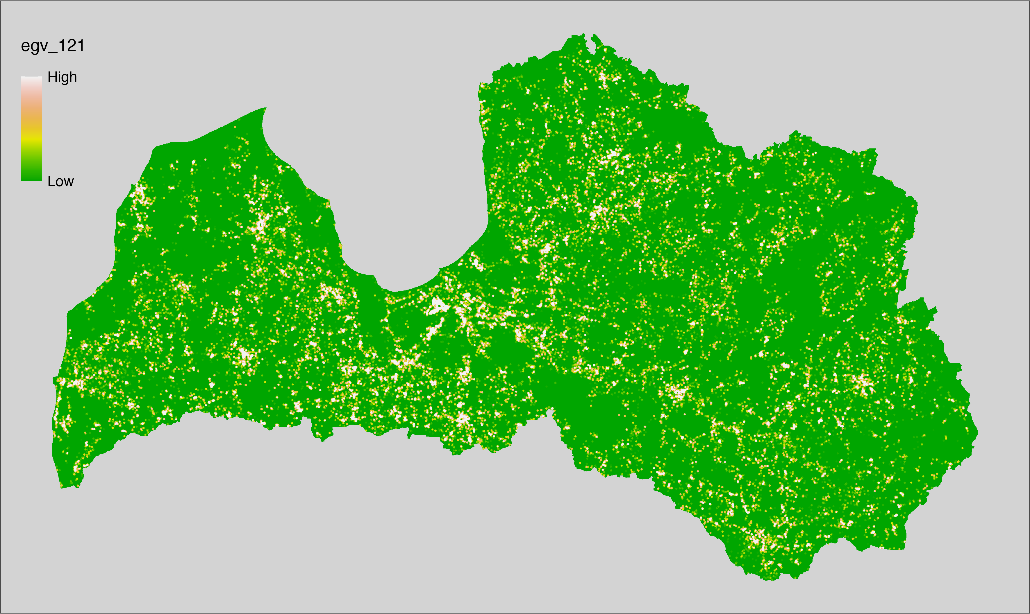
6.122 Edges_Farmland-Builtup_r1250
filename: Edges_Farmland-Builtup_r1250.tif
layername: egv_122
English name: Edge pixels of Farmland bordering with Built-Up areas within the 1.25 km landscape
Latvian name: Lauksaimniecības zemju malu ar apbūvi pikseļu skaits 1,25 km ainavā
Procedure: The total edge within a 1250 m radius around the analysis grid cell is
calculated as the area-weighted sum of the analysis cells inside the
buffer, using the workflow egvtools::radius_function(). During the calculation of the landscape metric,
inverse distance weighted (power = 2) gap filling on the output is applied
to ensure no missing values at the edges. Then the layer is rewritten to set
its name. Finally, the layer is standardised by subtracting the arithmetic
mean and dividing by the root mean squared error.
Code
# libs ----
if(!require(terra)) {install.packages("terra"); require(terra)}
if(!require(egvtools)) {remotes::install_github("aavotins/egvtools"); require(egvtools)}
# Templates -----
template100=rast("./Templates/TemplateRasters/LV100m_10km.tif")
# radii ----
radius_function(
kvadrati_path = "./Templates/TemplateGrids/tiles/",
radii_path = "./Templates/TemplateGridPoints/tiles/",
tikls100_path = "./Templates/TemplateGrids/tikls100_sauzeme.parquet",
template_path = "./Templates/TemplateRasters/LV100m_10km.tif",
input_layers = c("./RasterGrids_100m/2024/RAW/Edges_Farmland-Builtup_cell.tif"),
layer_prefixes = c("Edges_Farmland-Builtup"),
output_dir = "./RasterGrids_100m/2024/RAW/",
n_workers = 12,
radii = c("r1250"),
radius_mode = "sparse",
extract_fun = "sum",
fill_missing = TRUE,
IDW_weight = 2,
future_max_size = 20 * 1024^3)
# Edges_Farmland-Builtup_r1250.tif egv_122 ----
slanis=rast("./RasterGrids_100m/2024/RAW/Edges_Farmland-Builtup_r1250.tif")
names(slanis)="egv_122"
slanis2=project(slanis,template100)
writeRaster(slanis2,
"./RasterGrids_100m/2024/RAW/Edges_Farmland-Builtup_r1250.tif",
overwrite=TRUE)
# standardisation ----
if(!require(terra)) {install.packages("terra"); require(terra)}
if(!require(tidyverse)) {install.packages("tidyverse"); require(tidyverse)}
nosaukums="Edges_Farmland-Builtup_r1250.tif"
ielasisanas_cels=paste0("./RasterGrids_100m/2024/RAW/",nosaukums)
saglabasanas_cels=paste0("./RasterGrids_100m/2024/Scaled/",nosaukums)
slanis=rast(ielasisanas_cels)
videjais=global(slanis,fun="mean",na.rm=TRUE)
centrets=slanis-videjais[,1]
standartnovirze=terra::global(centrets,fun="rms",na.rm=TRUE)
merogots=centrets/standartnovirze[,1]
writeRaster(merogots,
filename=saglabasanas_cels,
overwrite=TRUE)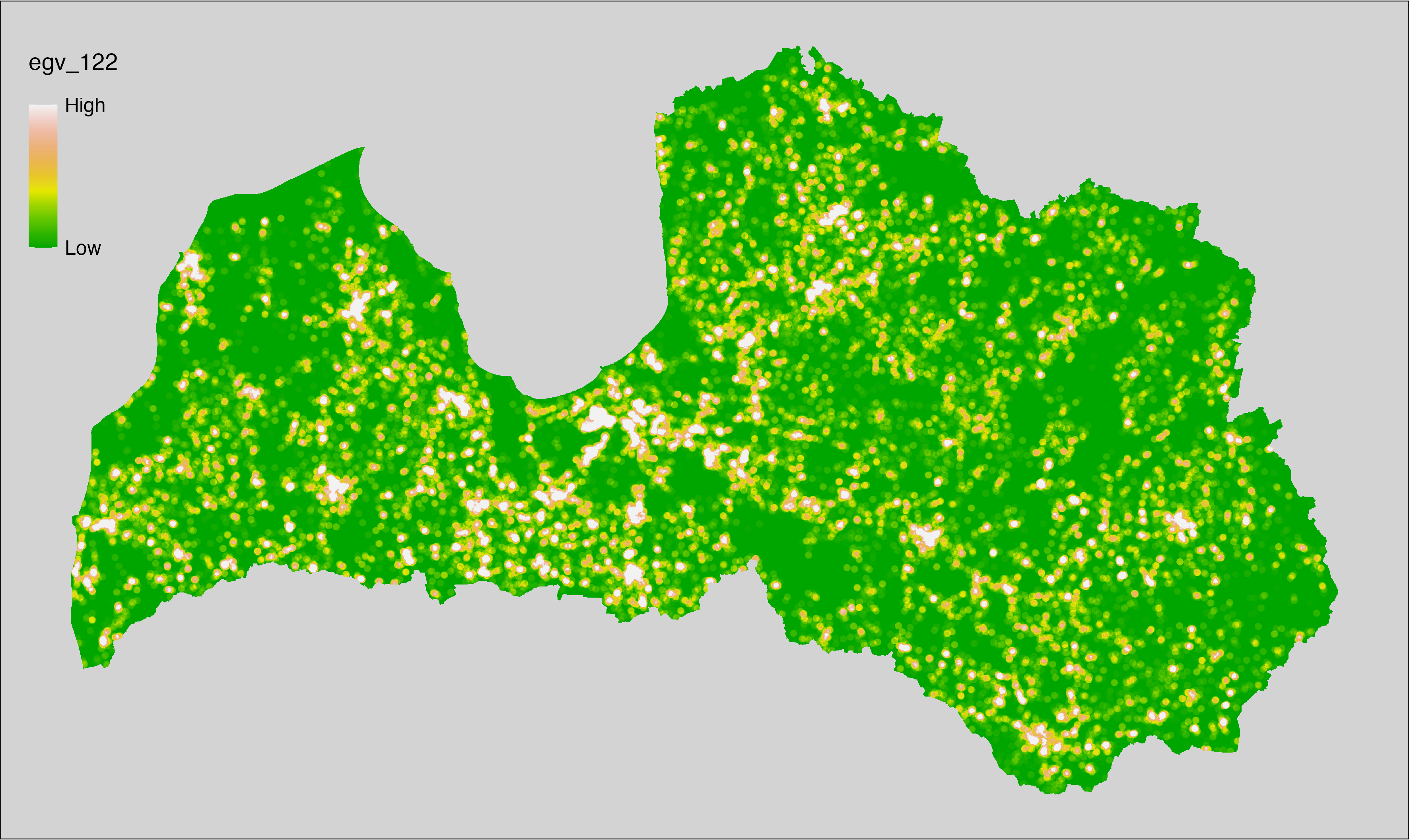
6.123 Edges_Farmland-Builtup_r3000
filename: Edges_Farmland-Builtup_r3000.tif
layername: egv_123
English name: Edge pixels of Farmland bordering with Built-Up areas within the 3 km landscape
Latvian name: Lauksaimniecības zemju malu ar apbūvi pikseļu skaits 3 km ainavā
Procedure: The total edge within a 3000 m radius around the analysis grid cell is
calculated as the area-weighted sum of the analysis cells inside the
buffer, using the workflow egvtools::radius_function(). During the calculation of the landscape metric,
inverse distance weighted (power = 2) gap filling on the output is applied
to ensure no missing values at the edges. Then the layer is rewritten to set
its name. Finally, the layer is standardised by subtracting the arithmetic
mean and dividing by the root mean squared error.
Code
# libs ----
if(!require(terra)) {install.packages("terra"); require(terra)}
if(!require(egvtools)) {remotes::install_github("aavotins/egvtools"); require(egvtools)}
# Templates -----
template100=rast("./Templates/TemplateRasters/LV100m_10km.tif")
# radii ----
radius_function(
kvadrati_path = "./Templates/TemplateGrids/tiles/",
radii_path = "./Templates/TemplateGridPoints/tiles/",
tikls100_path = "./Templates/TemplateGrids/tikls100_sauzeme.parquet",
template_path = "./Templates/TemplateRasters/LV100m_10km.tif",
input_layers = c("./RasterGrids_100m/2024/RAW/Edges_Farmland-Builtup_cell.tif"),
layer_prefixes = c("Edges_Farmland-Builtup"),
output_dir = "./RasterGrids_100m/2024/RAW/",
n_workers = 12,
radii = c("r3000"),
radius_mode = "sparse",
extract_fun = "sum",
fill_missing = TRUE,
IDW_weight = 2,
future_max_size = 20 * 1024^3)
# Edges_Farmland-Builtup_r3000.tif egv_123 ----
slanis=rast("./RasterGrids_100m/2024/RAW/Edges_Farmland-Builtup_r3000.tif")
names(slanis)="egv_123"
slanis2=project(slanis,template100)
writeRaster(slanis2,
"./RasterGrids_100m/2024/RAW/Edges_Farmland-Builtup_r3000.tif",
overwrite=TRUE)
# standardisation ----
if(!require(terra)) {install.packages("terra"); require(terra)}
if(!require(tidyverse)) {install.packages("tidyverse"); require(tidyverse)}
nosaukums="Edges_Farmland-Builtup_r3000.tif"
ielasisanas_cels=paste0("./RasterGrids_100m/2024/RAW/",nosaukums)
saglabasanas_cels=paste0("./RasterGrids_100m/2024/Scaled/",nosaukums)
slanis=rast(ielasisanas_cels)
videjais=global(slanis,fun="mean",na.rm=TRUE)
centrets=slanis-videjais[,1]
standartnovirze=terra::global(centrets,fun="rms",na.rm=TRUE)
merogots=centrets/standartnovirze[,1]
writeRaster(merogots,
filename=saglabasanas_cels,
overwrite=TRUE)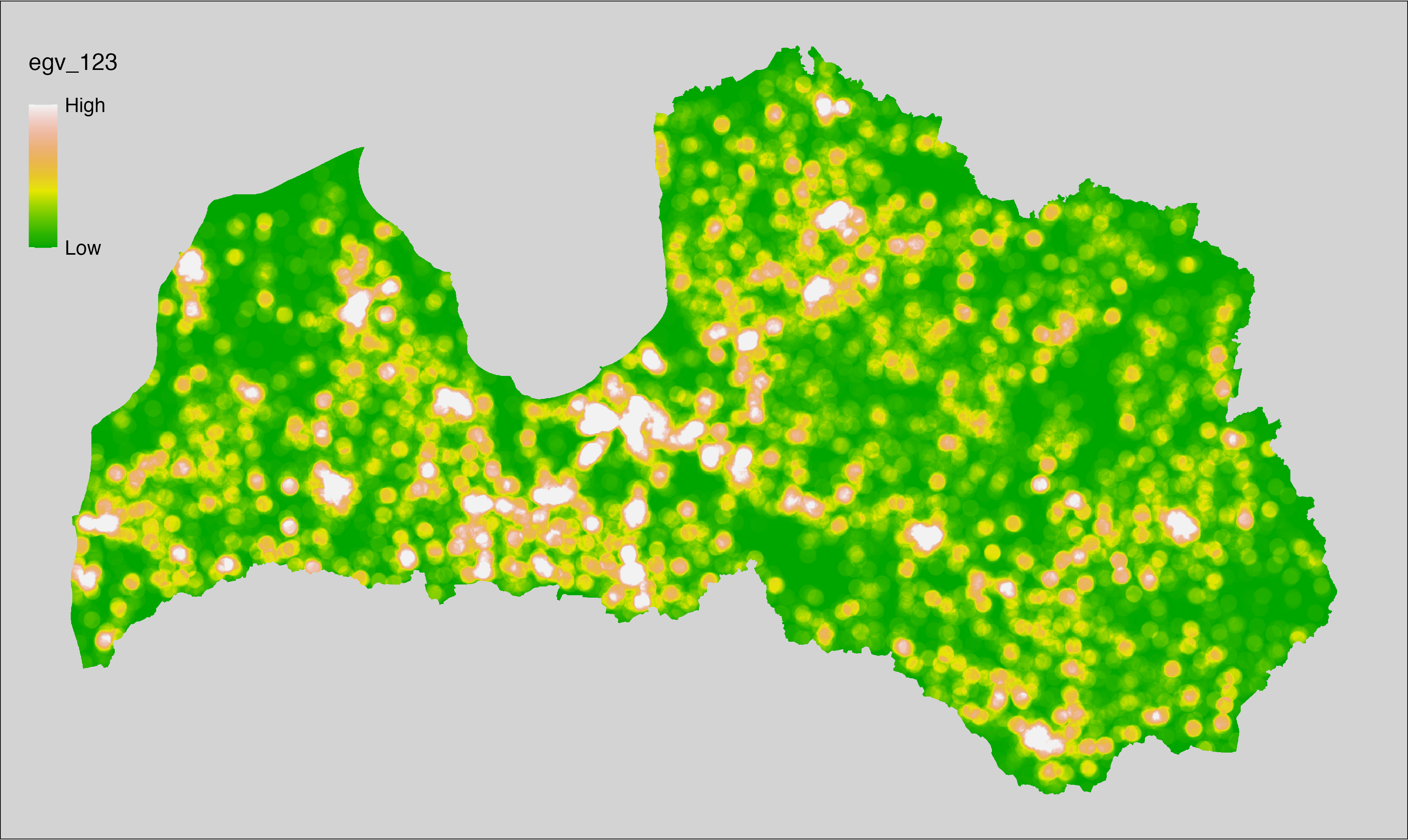
6.124 Edges_Farmland-Builtup_r10000
filename: Edges_Farmland-Builtup_r10000.tif
layername: egv_124
English name: Edge pixels of Farmland bordering with Built-Up areas within the 10 km landscape
Latvian name: Lauksaimniecības zemju malu ar apbūvi pikseļu skaits 10 km ainavā
Procedure: The total edge within a 10000 m radius around the analysis grid cell is
calculated as the area-weighted sum of the analysis cells inside the
buffer, using the workflow egvtools::radius_function(). During the calculation of the landscape metric,
inverse distance weighted (power = 2) gap filling on the output is applied
to ensure no missing values at the edges. Then the layer is rewritten to set
its name. Finally, the layer is standardised by subtracting the arithmetic
mean and dividing by the root mean squared error.
Code
# libs ----
if(!require(terra)) {install.packages("terra"); require(terra)}
if(!require(egvtools)) {remotes::install_github("aavotins/egvtools"); require(egvtools)}
# Templates -----
template100=rast("./Templates/TemplateRasters/LV100m_10km.tif")
# radii ----
radius_function(
kvadrati_path = "./Templates/TemplateGrids/tiles/",
radii_path = "./Templates/TemplateGridPoints/tiles/",
tikls100_path = "./Templates/TemplateGrids/tikls100_sauzeme.parquet",
template_path = "./Templates/TemplateRasters/LV100m_10km.tif",
input_layers = c("./RasterGrids_100m/2024/RAW/Edges_Farmland-Builtup_cell.tif"),
layer_prefixes = c("Edges_Farmland-Builtup"),
output_dir = "./RasterGrids_100m/2024/RAW/",
n_workers = 12,
radii = c("r10000"),
radius_mode = "sparse",
extract_fun = "sum",
fill_missing = TRUE,
IDW_weight = 2,
future_max_size = 20 * 1024^3)
# Edges_Farmland-Builtup_r10000.tif egv_124 ----
slanis=rast("./RasterGrids_100m/2024/RAW/Edges_Farmland-Builtup_r10000.tif")
names(slanis)="egv_124"
slanis2=project(slanis,template100)
writeRaster(slanis2,
"./RasterGrids_100m/2024/RAW/Edges_Farmland-Builtup_r10000.tif",
overwrite=TRUE)
# standardisation ----
if(!require(terra)) {install.packages("terra"); require(terra)}
if(!require(tidyverse)) {install.packages("tidyverse"); require(tidyverse)}
nosaukums="Edges_Farmland-Builtup_r10000.tif"
ielasisanas_cels=paste0("./RasterGrids_100m/2024/RAW/",nosaukums)
saglabasanas_cels=paste0("./RasterGrids_100m/2024/Scaled/",nosaukums)
slanis=rast(ielasisanas_cels)
videjais=global(slanis,fun="mean",na.rm=TRUE)
centrets=slanis-videjais[,1]
standartnovirze=terra::global(centrets,fun="rms",na.rm=TRUE)
merogots=centrets/standartnovirze[,1]
writeRaster(merogots,
filename=saglabasanas_cels,
overwrite=TRUE)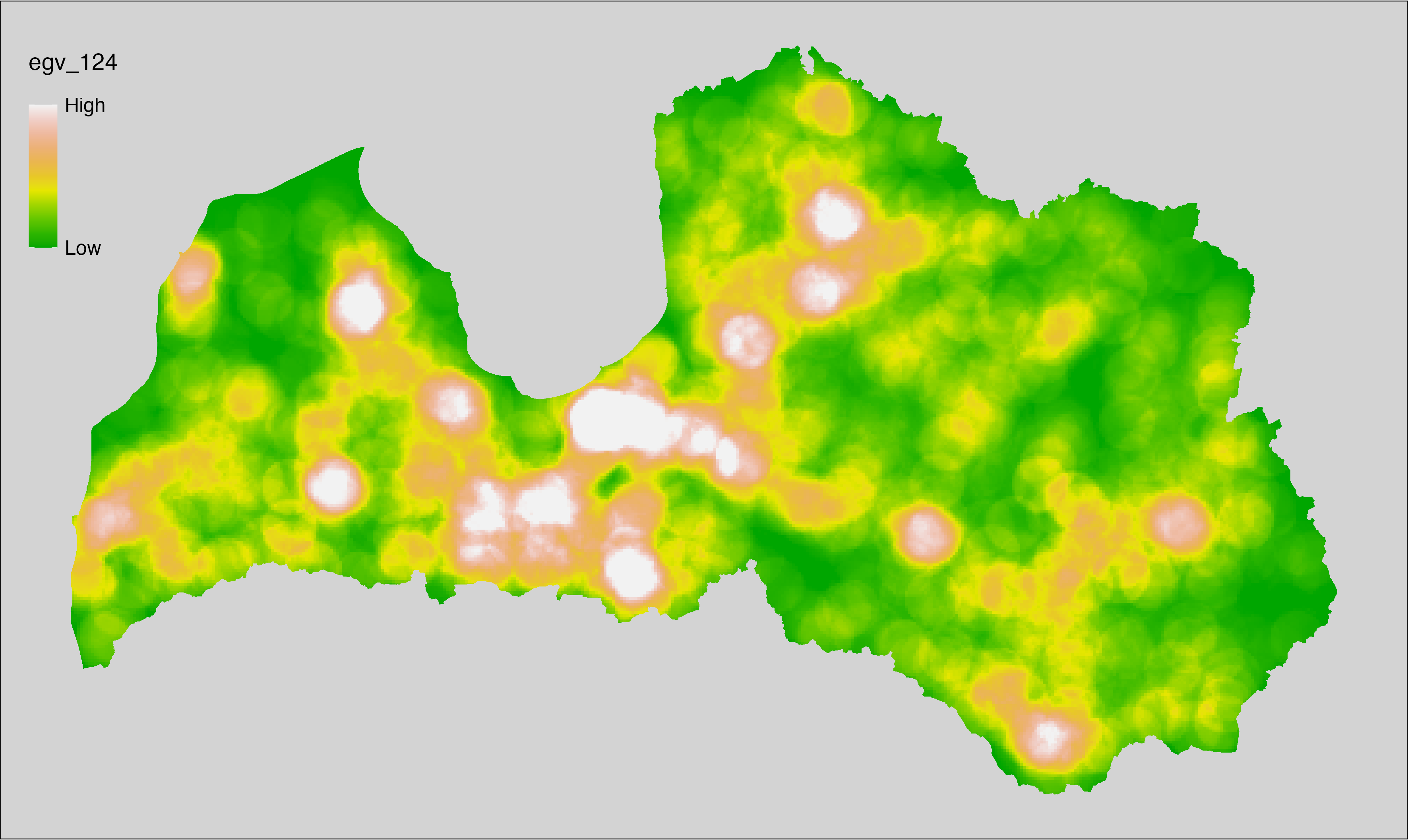
6.125 Edges_Trees-Builtup_cell
filename: Edges_Trees-Builtup_cell.tif
layername: egv_125
English name: Edge pixels of Trees bordering with Built-Up areas within the analysis cell (1 ha)
Latvian name: Koku malu ar apbūvi pikseļu skaits analīzes šūnā (1 ha)
Procedure: First, values larger than 630 and smaller than 700 from
Landscape classification are coded as 1, and other values as NA.
Then values 500 from the Landscape classification are coded as 0, and
other values as NA. Then, the first layer (1 = presence) is covered over the
second layer (presence = 0) and written to file (matching the input). Next,
using the workflow egvtools::landscape_function() total edge between the two
classes is calculated. During the calculation of the landscape metric, inverse distance
weighted (power = 2) gap filling on the output is applied to ensure no
missing values at the edges. Finally, the layer is standardised by
subtracting the arithmetic mean and dividing by the root mean squared error.
Code
# libs ----
if(!require(terra)) {install.packages("terra"); require(terra)}
if(!require(egvtools)) {remotes::install_github("aavotins/egvtools"); require(egvtools)}
if(!require(sf)) {install.packages("sf"); require(sf)}
if(!require(sfarrow)) {install.packages("sfarrow"); require(sfarrow)}
if(!require(raster)) {install.packages("raster"); require(raster)}
if(!require(fasterize)) {install.packages("fasterize"); require(fasterize)}
if(!require(tidyverse)) {install.packages("tidyverse"); require(tidyverse)}
# Templates -----
template10=rast("./Templates/TemplateRasters/LV10m_10km.tif")
nulls10=rast("./Templates/TemplateRasters/nulls_LV10m_10km.tif")
# simple landscape ----
simple_landscape=rast("./RasterGrids_10m/2024/Ainava_vienk_mask.tif")
# Edges_Trees-Builtup_input.tif ----
trees_from630=ifel(simple_landscape>=630 & simple_landscape<700,1,NA)
plot(trees_from630)
builtup=ifel(simple_landscape==500,0,NA)
plot(builtup)
trees630_builtup=cover(trees_from630,builtup)
plot(trees630_builtup)
edge_trees630_builtup=project(trees630_builtup,template10,
filename="./RasterGrids_10m/2024/Edges_Trees-Builtup_input.tif",
overwrite=TRUE)
rm(edge_trees630_builtup)
rm(trees630_builtup)
# Edges_Trees-Builtup_cell.tif egv_125 ----
landscape_function(
landscape = "./RasterGrids_10m/2024/Edges_Trees-Builtup_input.tif",
zones = "./Templates/TemplateGrids/tikls100_sauzeme.parquet",
id_field = "id",
tile_field = "tks50km",
template = "./Templates/TemplateRasters/LV100m_10km.tif",
out_dir = "./RasterGrids_100m/2024/RAW",
out_filename = "Edges_Trees-Builtup_cell.tif",
out_layername = "egv_125",
what = "lsm_l_te",
lm_args = list(count_boundary = FALSE),
rasterize_engine = "fasterize",
n_workers = 12,
future_max_size = 20 * 1024^3,
fill_gaps = TRUE,
plot_gaps = FALSE,
plot_result = FALSE
)
# standardisation ----
if(!require(terra)) {install.packages("terra"); require(terra)}
if(!require(tidyverse)) {install.packages("tidyverse"); require(tidyverse)}
nosaukums="Edges_Trees-Builtup_cell.tif"
ielasisanas_cels=paste0("./RasterGrids_100m/2024/RAW/",nosaukums)
saglabasanas_cels=paste0("./RasterGrids_100m/2024/Scaled/",nosaukums)
slanis=rast(ielasisanas_cels)
videjais=global(slanis,fun="mean",na.rm=TRUE)
centrets=slanis-videjais[,1]
standartnovirze=terra::global(centrets,fun="rms",na.rm=TRUE)
merogots=centrets/standartnovirze[,1]
writeRaster(merogots,
filename=saglabasanas_cels,
overwrite=TRUE)
6.126 Edges_Trees-Builtup_r500
filename: Edges_Trees-Builtup_r500.tif
layername: egv_126
English name: Edge pixels of Trees bordering with Built-Up areas within the 0.5 km landscape
Latvian name: Koku malu ar apbūvi pikseļu skaits 0,5 km ainavā
Procedure: The total edge within a 500 m radius around the analysis grid cell is
calculated as the area-weighted sum of the analysis cells inside the
buffer, using the workflow egvtools::radius_function(). During the calculation of the landscape metric,
inverse distance weighted (power = 2) gap filling on the output is applied
to ensure no missing values at the edges. Then the layer is rewritten to set
its name. Finally, the layer is standardised by subtracting the arithmetic
mean and dividing by the root mean squared error.
Code
# libs ----
if(!require(terra)) {install.packages("terra"); require(terra)}
if(!require(egvtools)) {remotes::install_github("aavotins/egvtools"); require(egvtools)}
# Templates -----
template100=rast("./Templates/TemplateRasters/LV100m_10km.tif")
# radii ----
radius_function(
kvadrati_path = "./Templates/TemplateGrids/tiles/",
radii_path = "./Templates/TemplateGridPoints/tiles/",
tikls100_path = "./Templates/TemplateGrids/tikls100_sauzeme.parquet",
template_path = "./Templates/TemplateRasters/LV100m_10km.tif",
input_layers = c("./RasterGrids_100m/2024/RAW/Edges_Trees-Builtup_cell.tif"),
layer_prefixes = c("Edges_Trees-Builtup"),
output_dir = "./RasterGrids_100m/2024/RAW/",
n_workers = 12,
radii = c("r500"),
radius_mode = "sparse",
extract_fun = "sum",
fill_missing = TRUE,
IDW_weight = 2,
future_max_size = 20 * 1024^3)
# Edges_Trees-Builtup_r500.tif egv_126 ----
slanis=rast("./RasterGrids_100m/2024/RAW/Edges_Trees-Builtup_r500.tif")
names(slanis)="egv_126"
slanis2=project(slanis,template100)
writeRaster(slanis2,
"./RasterGrids_100m/2024/RAW/Edges_Trees-Builtup_r500.tif",
overwrite=TRUE)
# standardisation ----
if(!require(terra)) {install.packages("terra"); require(terra)}
if(!require(tidyverse)) {install.packages("tidyverse"); require(tidyverse)}
nosaukums="Edges_Trees-Builtup_r500.tif"
ielasisanas_cels=paste0("./RasterGrids_100m/2024/RAW/",nosaukums)
saglabasanas_cels=paste0("./RasterGrids_100m/2024/Scaled/",nosaukums)
slanis=rast(ielasisanas_cels)
videjais=global(slanis,fun="mean",na.rm=TRUE)
centrets=slanis-videjais[,1]
standartnovirze=terra::global(centrets,fun="rms",na.rm=TRUE)
merogots=centrets/standartnovirze[,1]
writeRaster(merogots,
filename=saglabasanas_cels,
overwrite=TRUE)
6.127 Edges_Trees-Builtup_r1250
filename: Edges_Trees-Builtup_r1250.tif
layername: egv_127
English name: Edge pixels of Trees bordering with Built-Up areas within the 1.25 km landscape
Latvian name: Koku malu ar apbūvi pikseļu skaits 1,25 km ainavā
Procedure: The total edge within a 1250 m radius around the analysis grid cell is
calculated as the area-weighted sum of the analysis cells inside the
buffer, using the workflow egvtools::radius_function(). During the calculation of the landscape metric,
inverse distance weighted (power = 2) gap filling on the output is applied
to ensure no missing values at the edges. Then the layer is rewritten to set
its name. Finally, the layer is standardised by subtracting the arithmetic
mean and dividing by the root mean squared error.
Code
# libs ----
if(!require(terra)) {install.packages("terra"); require(terra)}
if(!require(egvtools)) {remotes::install_github("aavotins/egvtools"); require(egvtools)}
# Templates -----
template100=rast("./Templates/TemplateRasters/LV100m_10km.tif")
# radii ----
radius_function(
kvadrati_path = "./Templates/TemplateGrids/tiles/",
radii_path = "./Templates/TemplateGridPoints/tiles/",
tikls100_path = "./Templates/TemplateGrids/tikls100_sauzeme.parquet",
template_path = "./Templates/TemplateRasters/LV100m_10km.tif",
input_layers = c("./RasterGrids_100m/2024/RAW/Edges_Trees-Builtup_cell.tif"),
layer_prefixes = c("Edges_Trees-Builtup"),
output_dir = "./RasterGrids_100m/2024/RAW/",
n_workers = 12,
radii = c("r1250"),
radius_mode = "sparse",
extract_fun = "sum",
fill_missing = TRUE,
IDW_weight = 2,
future_max_size = 20 * 1024^3)
# Edges_Trees-Builtup_r1250.tif egv_127 ----
slanis=rast("./RasterGrids_100m/2024/RAW/Edges_Trees-Builtup_r1250.tif")
names(slanis)="egv_127"
slanis2=project(slanis,template100)
writeRaster(slanis2,
"./RasterGrids_100m/2024/RAW/Edges_Trees-Builtup_r1250.tif",
overwrite=TRUE)
# standardisation ----
if(!require(terra)) {install.packages("terra"); require(terra)}
if(!require(tidyverse)) {install.packages("tidyverse"); require(tidyverse)}
nosaukums="Edges_Trees-Builtup_r1250.tif"
ielasisanas_cels=paste0("./RasterGrids_100m/2024/RAW/",nosaukums)
saglabasanas_cels=paste0("./RasterGrids_100m/2024/Scaled/",nosaukums)
slanis=rast(ielasisanas_cels)
videjais=global(slanis,fun="mean",na.rm=TRUE)
centrets=slanis-videjais[,1]
standartnovirze=terra::global(centrets,fun="rms",na.rm=TRUE)
merogots=centrets/standartnovirze[,1]
writeRaster(merogots,
filename=saglabasanas_cels,
overwrite=TRUE)
6.128 Edges_Trees-Builtup_r3000
filename: Edges_Trees-Builtup_r3000.tif
layername: egv_128
English name: Edge pixels of Trees bordering with Built-Up areas within the 3 km landscape
Latvian name: Koku malu ar apbūvi pikseļu skaits 3 km ainavā
Procedure: The total edge within a 3000 m radius around the analysis grid cell is
calculated as the area-weighted sum of the analysis cells inside the
buffer, using the workflow egvtools::radius_function(). During the calculation of the landscape metric,
inverse distance weighted (power = 2) gap filling on the output is applied
to ensure no missing values at the edges. Then the layer is rewritten to set
its name. Finally, the layer is standardised by subtracting the arithmetic
mean and dividing by the root mean squared error.
Code
# libs ----
if(!require(terra)) {install.packages("terra"); require(terra)}
if(!require(egvtools)) {remotes::install_github("aavotins/egvtools"); require(egvtools)}
# Templates -----
template100=rast("./Templates/TemplateRasters/LV100m_10km.tif")
# radii ----
radius_function(
kvadrati_path = "./Templates/TemplateGrids/tiles/",
radii_path = "./Templates/TemplateGridPoints/tiles/",
tikls100_path = "./Templates/TemplateGrids/tikls100_sauzeme.parquet",
template_path = "./Templates/TemplateRasters/LV100m_10km.tif",
input_layers = c("./RasterGrids_100m/2024/RAW/Edges_Trees-Builtup_cell.tif"),
layer_prefixes = c("Edges_Trees-Builtup"),
output_dir = "./RasterGrids_100m/2024/RAW/",
n_workers = 12,
radii = c("r3000"),
radius_mode = "sparse",
extract_fun = "sum",
fill_missing = TRUE,
IDW_weight = 2,
future_max_size = 20 * 1024^3)
# Edges_Trees-Builtup_r3000.tif egv_128 ----
slanis=rast("./RasterGrids_100m/2024/RAW/Edges_Trees-Builtup_r3000.tif")
names(slanis)="egv_128"
slanis2=project(slanis,template100)
writeRaster(slanis2,
"./RasterGrids_100m/2024/RAW/Edges_Trees-Builtup_r3000.tif",
overwrite=TRUE)
# standardisation ----
if(!require(terra)) {install.packages("terra"); require(terra)}
if(!require(tidyverse)) {install.packages("tidyverse"); require(tidyverse)}
nosaukums="Edges_Trees-Builtup_r3000.tif"
ielasisanas_cels=paste0("./RasterGrids_100m/2024/RAW/",nosaukums)
saglabasanas_cels=paste0("./RasterGrids_100m/2024/Scaled/",nosaukums)
slanis=rast(ielasisanas_cels)
videjais=global(slanis,fun="mean",na.rm=TRUE)
centrets=slanis-videjais[,1]
standartnovirze=terra::global(centrets,fun="rms",na.rm=TRUE)
merogots=centrets/standartnovirze[,1]
writeRaster(merogots,
filename=saglabasanas_cels,
overwrite=TRUE)
6.129 Edges_Trees-Builtup_r10000
filename: Edges_Trees-Builtup_r10000.tif
layername: egv_129
English name: Edge pixels of Trees bordering with Built-Up areas within the 10 km landscape
Latvian name: Koku malu ar apbūvi pikseļu skaits 10 km ainavā
Procedure: The total edge within a 10000 m radius around the analysis grid cell is
calculated as the area-weighted sum of the analysis cells inside the
buffer, using the workflow egvtools::radius_function(). During the calculation of the landscape metric,
inverse distance weighted (power = 2) gap filling on the output is applied
to ensure no missing values at the edges. Then the layer is rewritten to set
its name. Finally, the layer is standardised by subtracting the arithmetic
mean and dividing by the root mean squared error.
Code
# libs ----
if(!require(terra)) {install.packages("terra"); require(terra)}
if(!require(egvtools)) {remotes::install_github("aavotins/egvtools"); require(egvtools)}
# Templates -----
template100=rast("./Templates/TemplateRasters/LV100m_10km.tif")
# radii ----
radius_function(
kvadrati_path = "./Templates/TemplateGrids/tiles/",
radii_path = "./Templates/TemplateGridPoints/tiles/",
tikls100_path = "./Templates/TemplateGrids/tikls100_sauzeme.parquet",
template_path = "./Templates/TemplateRasters/LV100m_10km.tif",
input_layers = c("./RasterGrids_100m/2024/RAW/Edges_Trees-Builtup_cell.tif"),
layer_prefixes = c("Edges_Trees-Builtup"),
output_dir = "./RasterGrids_100m/2024/RAW/",
n_workers = 12,
radii = c("r10000"),
radius_mode = "sparse",
extract_fun = "sum",
fill_missing = TRUE,
IDW_weight = 2,
future_max_size = 20 * 1024^3)
# Edges_Trees-Builtup_r10000.tif egv_129 ----
slanis=rast("./RasterGrids_100m/2024/RAW/Edges_Trees-Builtup_r10000.tif")
names(slanis)="egv_129"
slanis2=project(slanis,template100)
writeRaster(slanis2,
"./RasterGrids_100m/2024/RAW/Edges_Trees-Builtup_r10000.tif",
overwrite=TRUE)
# standardisation ----
if(!require(terra)) {install.packages("terra"); require(terra)}
if(!require(tidyverse)) {install.packages("tidyverse"); require(tidyverse)}
nosaukums="Edges_Trees-Builtup_r10000.tif"
ielasisanas_cels=paste0("./RasterGrids_100m/2024/RAW/",nosaukums)
saglabasanas_cels=paste0("./RasterGrids_100m/2024/Scaled/",nosaukums)
slanis=rast(ielasisanas_cels)
videjais=global(slanis,fun="mean",na.rm=TRUE)
centrets=slanis-videjais[,1]
standartnovirze=terra::global(centrets,fun="rms",na.rm=TRUE)
merogots=centrets/standartnovirze[,1]
writeRaster(merogots,
filename=saglabasanas_cels,
overwrite=TRUE)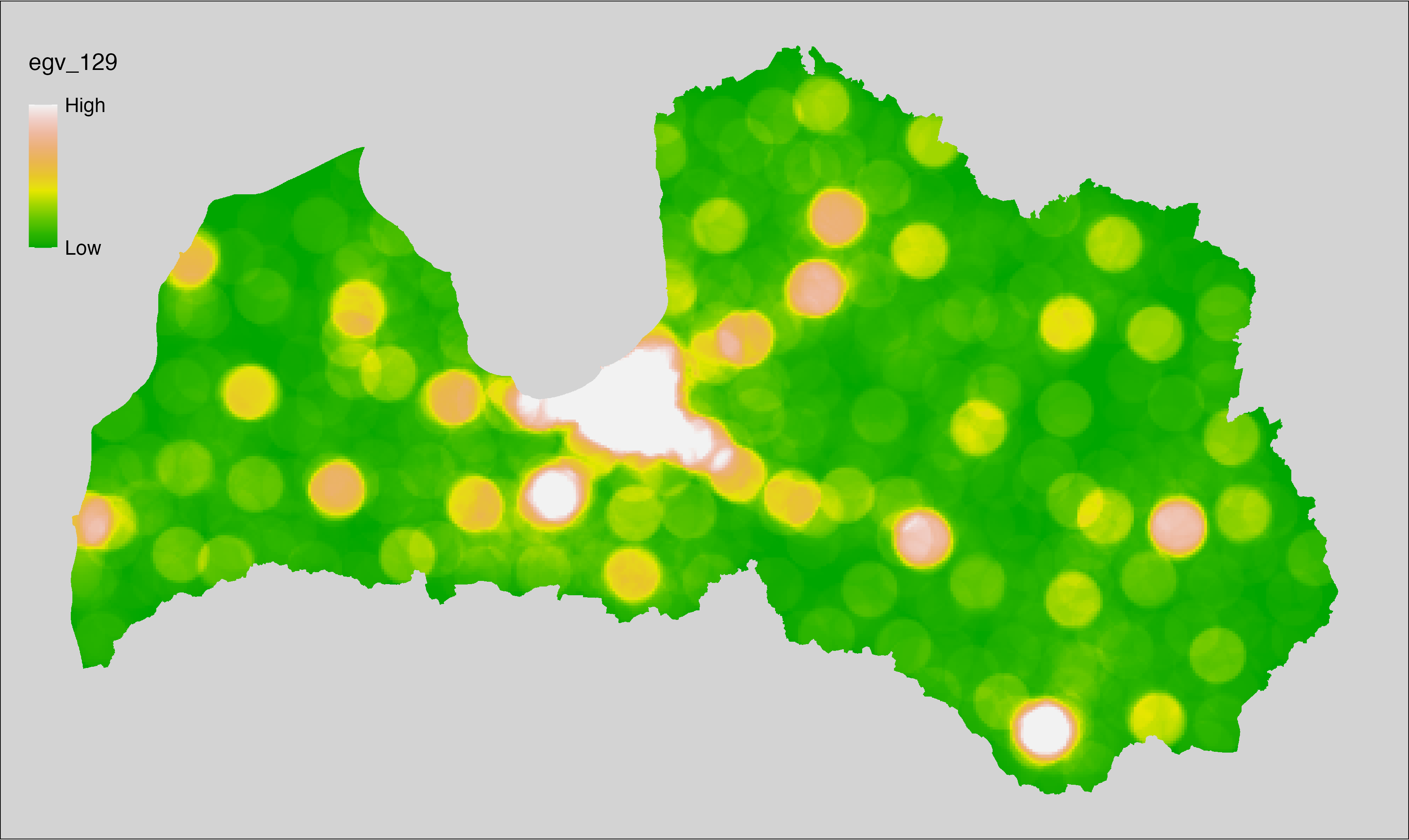
6.130 Edges_CropsFallow_cell
filename: Edges_CropsFallow_cell.tif
layername: egv_130
English name: Edge pixels of Cropland, Fallow land within the analysis cell (1 ha)
Latvian name: Aramzemju malu pikseļu skaits analīzes šūnā (1 ha)
Procedure: First, values larger than or equal to 310 and smaller than 325
from the Landscape classification are coded as 1, and all other values as
NA. Then, the layer (1 = presence) is covered over the nulls layer (presence = 0)
and written to file (matching the input). Next, using the workflow
egvtools::landscape_function() total edge between the two classes is
calculated. During the calculation of the landscape metric, inverse distance weighted
(power = 2) gap filling on the output is applied to ensure no missing values
at the edges. Finally, the layer is standardised by subtracting the arithmetic
mean and dividing by the root mean squared error.
Code
# libs ----
if(!require(terra)) {install.packages("terra"); require(terra)}
if(!require(egvtools)) {remotes::install_github("aavotins/egvtools"); require(egvtools)}
if(!require(sf)) {install.packages("sf"); require(sf)}
if(!require(sfarrow)) {install.packages("sfarrow"); require(sfarrow)}
if(!require(raster)) {install.packages("raster"); require(raster)}
if(!require(fasterize)) {install.packages("fasterize"); require(fasterize)}
if(!require(tidyverse)) {install.packages("tidyverse"); require(tidyverse)}
# Templates -----
template10=rast("./Templates/TemplateRasters/LV10m_10km.tif")
nulls10=rast("./Templates/TemplateRasters/nulls_LV10m_10km.tif")
# simple landscape ----
simple_landscape=rast("./RasterGrids_10m/2024/Ainava_vienk_mask.tif")
# Edges_CropsFallow_input.tif ----
cropsfallow=ifel(simple_landscape>=310 & simple_landscape<325,1,NA)
plot(cropsfallow)
cropsfallow=cover(cropsfallow,nulls10)
plot(cropsfallow)
edge_cropsfallow=project(cropsfallow,template10,
filename="./RasterGrids_10m/2024/Edges_CropsFallow_input.tif",
overwrite=TRUE)
rm(edge_cropsfallow)
# Edges_CropsFallow_cell.tif egv_130 ----
landscape_function(
landscape = "./RasterGrids_10m/2024/Edges_CropsFallow_input.tif",
zones = "./Templates/TemplateGrids/tikls100_sauzeme.parquet",
id_field = "id",
tile_field = "tks50km",
template = "./Templates/TemplateRasters/LV100m_10km.tif",
out_dir = "./RasterGrids_100m/2024/RAW",
out_filename = "Edges_CropsFallow_cell.tif",
out_layername = "egv_130",
what = "lsm_l_te",
lm_args = list(count_boundary = FALSE),
rasterize_engine = "fasterize",
n_workers = 12,
future_max_size = 20 * 1024^3,
fill_gaps = TRUE,
plot_gaps = FALSE,
plot_result = FALSE
)
# standardisation ----
if(!require(terra)) {install.packages("terra"); require(terra)}
if(!require(tidyverse)) {install.packages("tidyverse"); require(tidyverse)}
nosaukums="Edges_CropsFallow_cell.tif"
ielasisanas_cels=paste0("./RasterGrids_100m/2024/RAW/",nosaukums)
saglabasanas_cels=paste0("./RasterGrids_100m/2024/Scaled/",nosaukums)
slanis=rast(ielasisanas_cels)
videjais=global(slanis,fun="mean",na.rm=TRUE)
centrets=slanis-videjais[,1]
standartnovirze=terra::global(centrets,fun="rms",na.rm=TRUE)
merogots=centrets/standartnovirze[,1]
writeRaster(merogots,
filename=saglabasanas_cels,
overwrite=TRUE)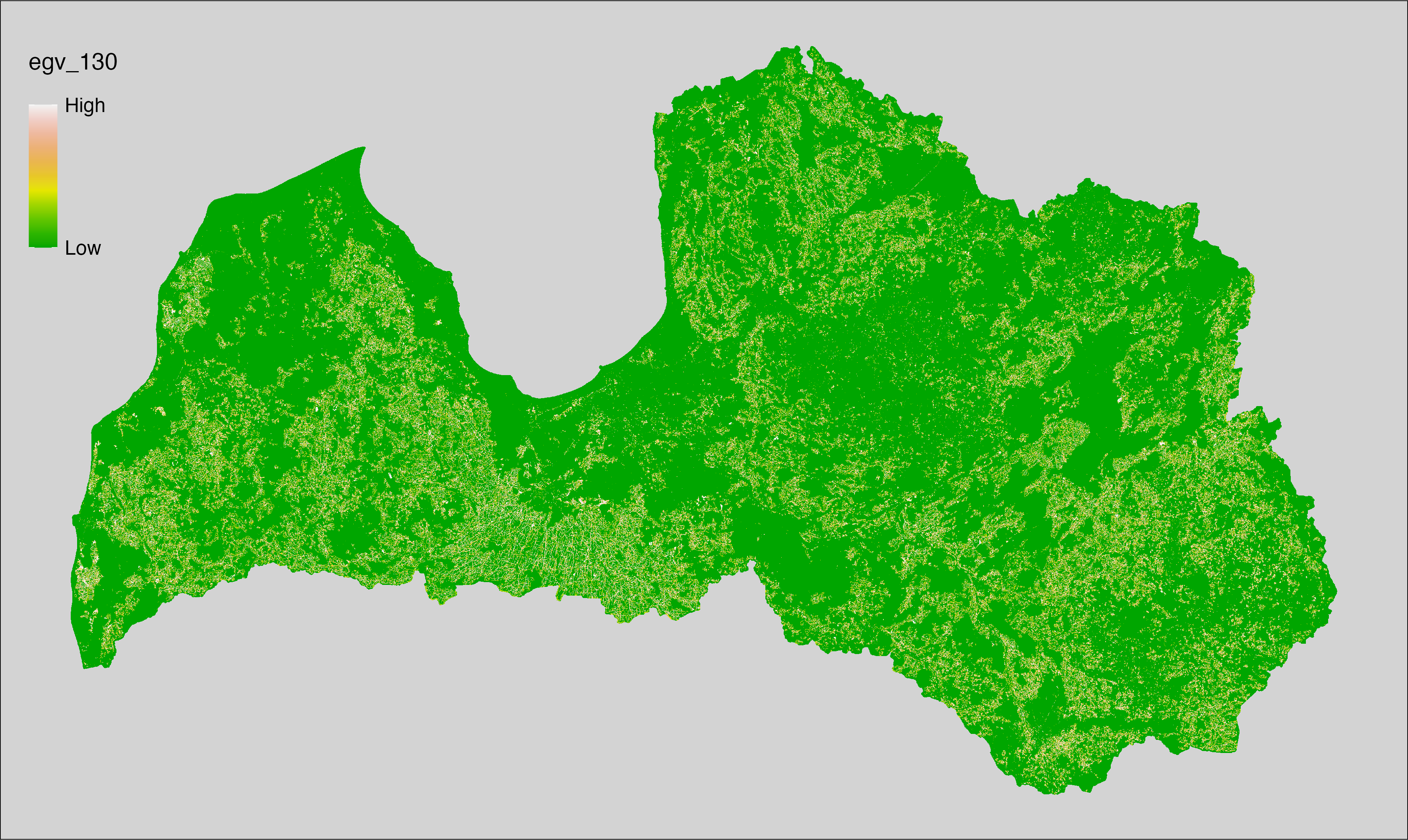
6.131 Edges_CropsFallow_r500
filename: Edges_CropsFallow_r500.tif
layername: egv_131
English name: Edge pixels of Cropland, Fallow land within the 0.5 km landscape
Latvian name: Aramzemju malu pikseļu skaits 0,5 km ainavā
Procedure: The total edge within a 500 m radius around the analysis grid cell is
calculated as the area-weighted sum of the analysis cells inside the
buffer, using the workflow egvtools::radius_function(). During the calculation of the landscape metric,
inverse distance weighted (power = 2) gap filling on the output is applied
to ensure no missing values at the edges. Then the layer is rewritten to set
its name. Finally, the layer is standardised by subtracting the arithmetic
mean and dividing by the root mean squared error.
Code
# libs ----
if(!require(terra)) {install.packages("terra"); require(terra)}
if(!require(egvtools)) {remotes::install_github("aavotins/egvtools"); require(egvtools)}
# Templates -----
template100=rast("./Templates/TemplateRasters/LV100m_10km.tif")
# radii ----
radius_function(
kvadrati_path = "./Templates/TemplateGrids/tiles/",
radii_path = "./Templates/TemplateGridPoints/tiles/",
tikls100_path = "./Templates/TemplateGrids/tikls100_sauzeme.parquet",
template_path = "./Templates/TemplateRasters/LV100m_10km.tif",
input_layers = c("./RasterGrids_100m/2024/RAW/Edges_CropsFallow_cell.tif"),
layer_prefixes = c("Edges_CropsFallow"),
output_dir = "./RasterGrids_100m/2024/RAW/",
n_workers = 12,
radii = c("r500"),
radius_mode = "sparse",
extract_fun = "sum",
fill_missing = TRUE,
IDW_weight = 2,
future_max_size = 20 * 1024^3)
# Edges_CropsFallow_r500.tif egv_131 ----
slanis=rast("./RasterGrids_100m/2024/RAW/Edges_CropsFallow_r500.tif")
names(slanis)="egv_131"
slanis2=project(slanis,template100)
writeRaster(slanis2,
"./RasterGrids_100m/2024/RAW/Edges_CropsFallow_r500.tif",
overwrite=TRUE)
# standardisation ----
if(!require(terra)) {install.packages("terra"); require(terra)}
if(!require(tidyverse)) {install.packages("tidyverse"); require(tidyverse)}
nosaukums="Edges_CropsFallow_r500.tif"
ielasisanas_cels=paste0("./RasterGrids_100m/2024/RAW/",nosaukums)
saglabasanas_cels=paste0("./RasterGrids_100m/2024/Scaled/",nosaukums)
slanis=rast(ielasisanas_cels)
videjais=global(slanis,fun="mean",na.rm=TRUE)
centrets=slanis-videjais[,1]
standartnovirze=terra::global(centrets,fun="rms",na.rm=TRUE)
merogots=centrets/standartnovirze[,1]
writeRaster(merogots,
filename=saglabasanas_cels,
overwrite=TRUE)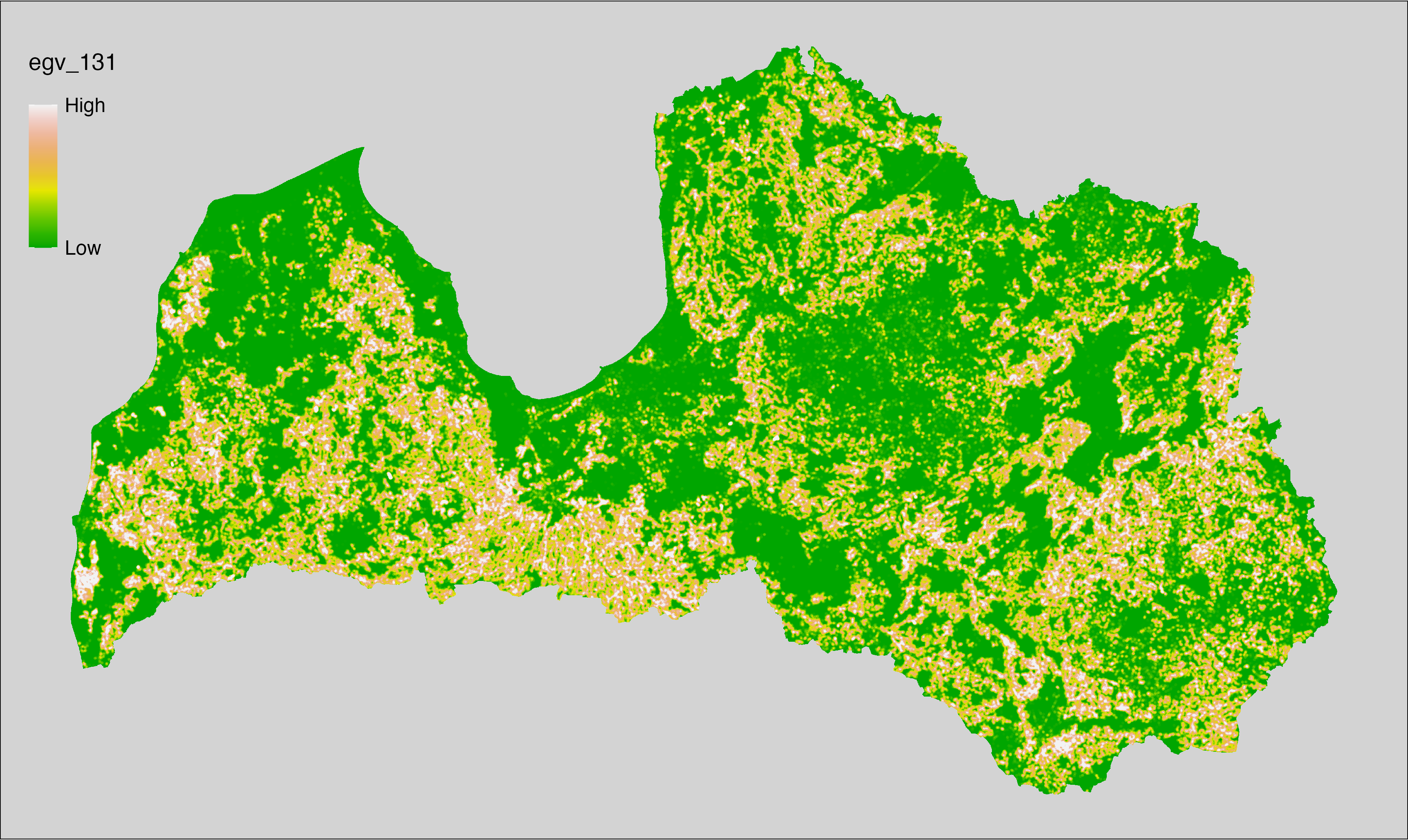
6.132 Edges_CropsFallow_r1250
filename: Edges_CropsFallow_r1250.tif
layername: egv_132
English name: Edge pixels of Cropland, Fallow land within the 1.25 km landscape
Latvian name: Aramzemju malu pikseļu skaits 1,25 km ainavā
Procedure: The total edge within a 1250 m radius around the analysis grid cell is
calculated as the area-weighted sum of the analysis cells inside the
buffer, using the workflow egvtools::radius_function(). During the calculation of the landscape metric,
inverse distance weighted (power = 2) gap filling on the output is applied
to ensure no missing values at the edges. Then the layer is rewritten to set
its name. Finally, the layer is standardised by subtracting the arithmetic
mean and dividing by the root mean squared error.
Code
# libs ----
if(!require(terra)) {install.packages("terra"); require(terra)}
if(!require(egvtools)) {remotes::install_github("aavotins/egvtools"); require(egvtools)}
# Templates -----
template100=rast("./Templates/TemplateRasters/LV100m_10km.tif")
# radii ----
radius_function(
kvadrati_path = "./Templates/TemplateGrids/tiles/",
radii_path = "./Templates/TemplateGridPoints/tiles/",
tikls100_path = "./Templates/TemplateGrids/tikls100_sauzeme.parquet",
template_path = "./Templates/TemplateRasters/LV100m_10km.tif",
input_layers = c("./RasterGrids_100m/2024/RAW/Edges_CropsFallow_cell.tif"),
layer_prefixes = c("Edges_CropsFallow"),
output_dir = "./RasterGrids_100m/2024/RAW/",
n_workers = 12,
radii = c("r1250"),
radius_mode = "sparse",
extract_fun = "sum",
fill_missing = TRUE,
IDW_weight = 2,
future_max_size = 20 * 1024^3)
# Edges_CropsFallow_r1250.tif egv_132 ----
slanis=rast("./RasterGrids_100m/2024/RAW/Edges_CropsFallow_r1250.tif")
names(slanis)="egv_132"
slanis2=project(slanis,template100)
writeRaster(slanis2,
"./RasterGrids_100m/2024/RAW/Edges_CropsFallow_r1250.tif",
overwrite=TRUE)
# standardisation ----
if(!require(terra)) {install.packages("terra"); require(terra)}
if(!require(tidyverse)) {install.packages("tidyverse"); require(tidyverse)}
nosaukums="Edges_CropsFallow_r1250.tif"
ielasisanas_cels=paste0("./RasterGrids_100m/2024/RAW/",nosaukums)
saglabasanas_cels=paste0("./RasterGrids_100m/2024/Scaled/",nosaukums)
slanis=rast(ielasisanas_cels)
videjais=global(slanis,fun="mean",na.rm=TRUE)
centrets=slanis-videjais[,1]
standartnovirze=terra::global(centrets,fun="rms",na.rm=TRUE)
merogots=centrets/standartnovirze[,1]
writeRaster(merogots,
filename=saglabasanas_cels,
overwrite=TRUE)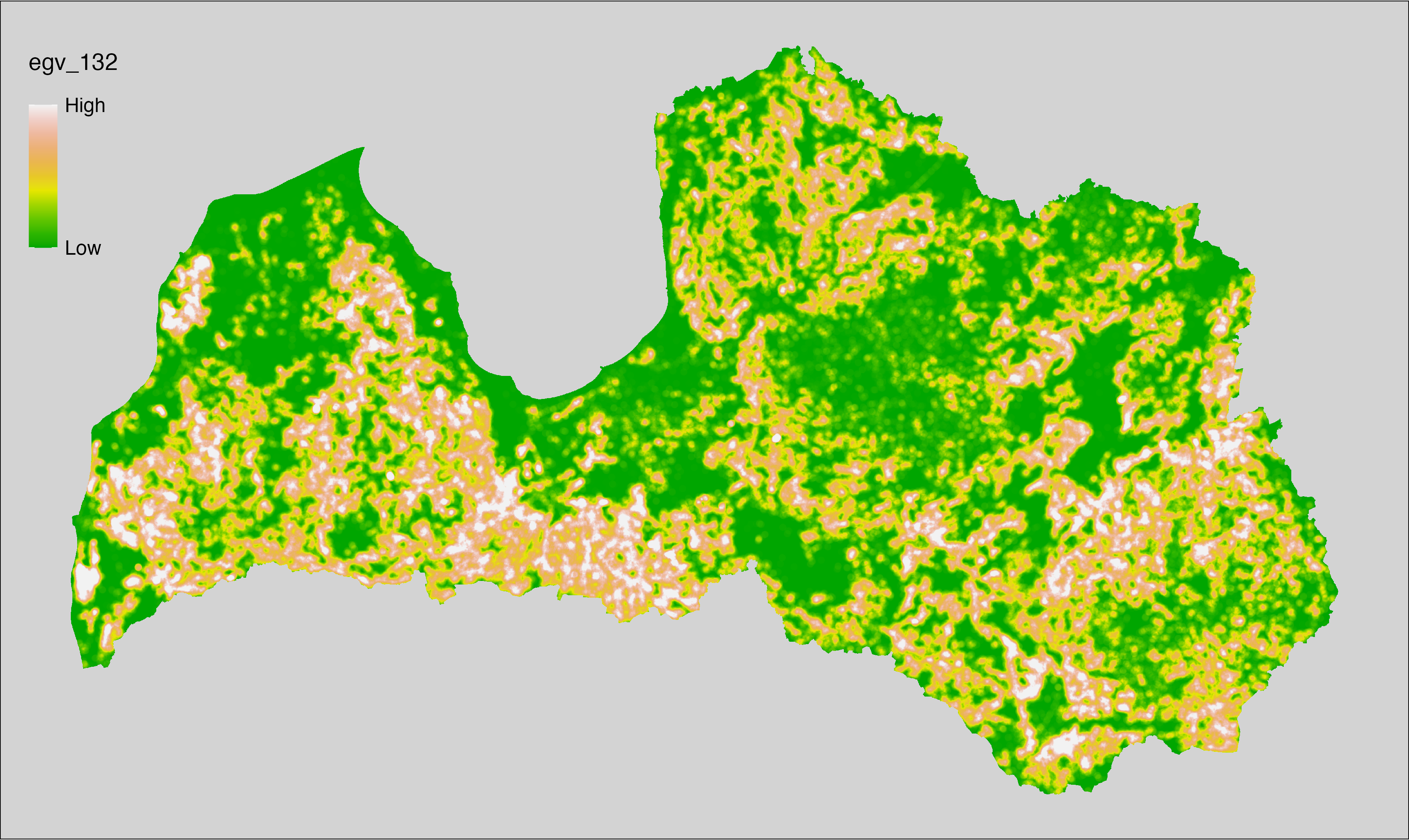
6.133 Edges_CropsFallow_r3000
filename: Edges_CropsFallow_r3000.tif
layername: egv_133
English name: Edge pixels of Cropland, Fallow land within the 3 km landscape
Latvian name: Aramzemju malu pikseļu skaits 3 km ainavā
Procedure: The total edge within a 3000 m radius around the analysis grid cell is
calculated as the area-weighted sum of the analysis cells inside the
buffer, using the workflow egvtools::radius_function(). During the calculation of the landscape metric,
inverse distance weighted (power = 2) gap filling on the output is applied
to ensure no missing values at the edges. Then the layer is rewritten to set
its name. Finally, the layer is standardised by subtracting the arithmetic
mean and dividing by the root mean squared error.
Code
# libs ----
if(!require(terra)) {install.packages("terra"); require(terra)}
if(!require(egvtools)) {remotes::install_github("aavotins/egvtools"); require(egvtools)}
# Templates -----
template100=rast("./Templates/TemplateRasters/LV100m_10km.tif")
# radii ----
radius_function(
kvadrati_path = "./Templates/TemplateGrids/tiles/",
radii_path = "./Templates/TemplateGridPoints/tiles/",
tikls100_path = "./Templates/TemplateGrids/tikls100_sauzeme.parquet",
template_path = "./Templates/TemplateRasters/LV100m_10km.tif",
input_layers = c("./RasterGrids_100m/2024/RAW/Edges_CropsFallow_cell.tif"),
layer_prefixes = c("Edges_CropsFallow"),
output_dir = "./RasterGrids_100m/2024/RAW/",
n_workers = 12,
radii = c("r3000"),
radius_mode = "sparse",
extract_fun = "sum",
fill_missing = TRUE,
IDW_weight = 2,
future_max_size = 20 * 1024^3)
# Edges_CropsFallow_r3000.tif egv_133 ----
slanis=rast("./RasterGrids_100m/2024/RAW/Edges_CropsFallow_r3000.tif")
names(slanis)="egv_133"
slanis2=project(slanis,template100)
writeRaster(slanis2,
"./RasterGrids_100m/2024/RAW/Edges_CropsFallow_r3000.tif",
overwrite=TRUE)
# standardisation ----
if(!require(terra)) {install.packages("terra"); require(terra)}
if(!require(tidyverse)) {install.packages("tidyverse"); require(tidyverse)}
nosaukums="Edges_CropsFallow_r3000.tif"
ielasisanas_cels=paste0("./RasterGrids_100m/2024/RAW/",nosaukums)
saglabasanas_cels=paste0("./RasterGrids_100m/2024/Scaled/",nosaukums)
slanis=rast(ielasisanas_cels)
videjais=global(slanis,fun="mean",na.rm=TRUE)
centrets=slanis-videjais[,1]
standartnovirze=terra::global(centrets,fun="rms",na.rm=TRUE)
merogots=centrets/standartnovirze[,1]
writeRaster(merogots,
filename=saglabasanas_cels,
overwrite=TRUE)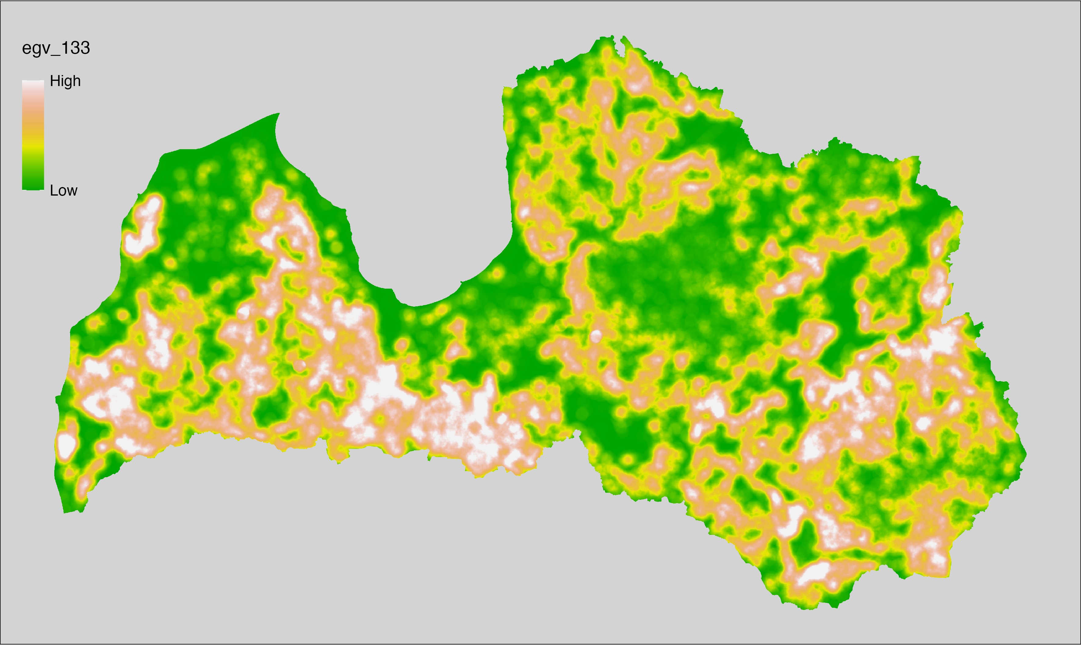
6.134 Edges_CropsFallow_r10000
filename: Edges_CropsFallow_r10000.tif
layername: egv_134
English name: Edge pixels of Cropland, Fallow land within the 10 km landscape
Latvian name: Aramzemju malu pikseļu skaits 10 km ainavā
Procedure: The total edge within a 10000 m radius around the analysis grid cell is
calculated as the area-weighted sum of the analysis cells inside the
buffer, using the workflow egvtools::radius_function(). During the calculation of the landscape metric,
inverse distance weighted (power = 2) gap filling on the output is applied
to ensure no missing values at the edges. Then the layer is rewritten to set
its name. Finally, the layer is standardised by subtracting the arithmetic
mean and dividing by the root mean squared error.
Code
# libs ----
if(!require(terra)) {install.packages("terra"); require(terra)}
if(!require(egvtools)) {remotes::install_github("aavotins/egvtools"); require(egvtools)}
# Templates -----
template100=rast("./Templates/TemplateRasters/LV100m_10km.tif")
# radii ----
radius_function(
kvadrati_path = "./Templates/TemplateGrids/tiles/",
radii_path = "./Templates/TemplateGridPoints/tiles/",
tikls100_path = "./Templates/TemplateGrids/tikls100_sauzeme.parquet",
template_path = "./Templates/TemplateRasters/LV100m_10km.tif",
input_layers = c("./RasterGrids_100m/2024/RAW/Edges_CropsFallow_cell.tif"),
layer_prefixes = c("Edges_CropsFallow"),
output_dir = "./RasterGrids_100m/2024/RAW/",
n_workers = 12,
radii = c("r10000"),
radius_mode = "sparse",
extract_fun = "sum",
fill_missing = TRUE,
IDW_weight = 2,
future_max_size = 20 * 1024^3)
# Edges_CropsFallow_r10000.tif egv_134 ----
slanis=rast("./RasterGrids_100m/2024/RAW/Edges_CropsFallow_r10000.tif")
names(slanis)="egv_134"
slanis2=project(slanis,template100)
writeRaster(slanis2,
"./RasterGrids_100m/2024/RAW/Edges_CropsFallow_r10000.tif",
overwrite=TRUE)
# standardisation ----
if(!require(terra)) {install.packages("terra"); require(terra)}
if(!require(tidyverse)) {install.packages("tidyverse"); require(tidyverse)}
nosaukums="Edges_CropsFallow_r10000.tif"
ielasisanas_cels=paste0("./RasterGrids_100m/2024/RAW/",nosaukums)
saglabasanas_cels=paste0("./RasterGrids_100m/2024/Scaled/",nosaukums)
slanis=rast(ielasisanas_cels)
videjais=global(slanis,fun="mean",na.rm=TRUE)
centrets=slanis-videjais[,1]
standartnovirze=terra::global(centrets,fun="rms",na.rm=TRUE)
merogots=centrets/standartnovirze[,1]
writeRaster(merogots,
filename=saglabasanas_cels,
overwrite=TRUE)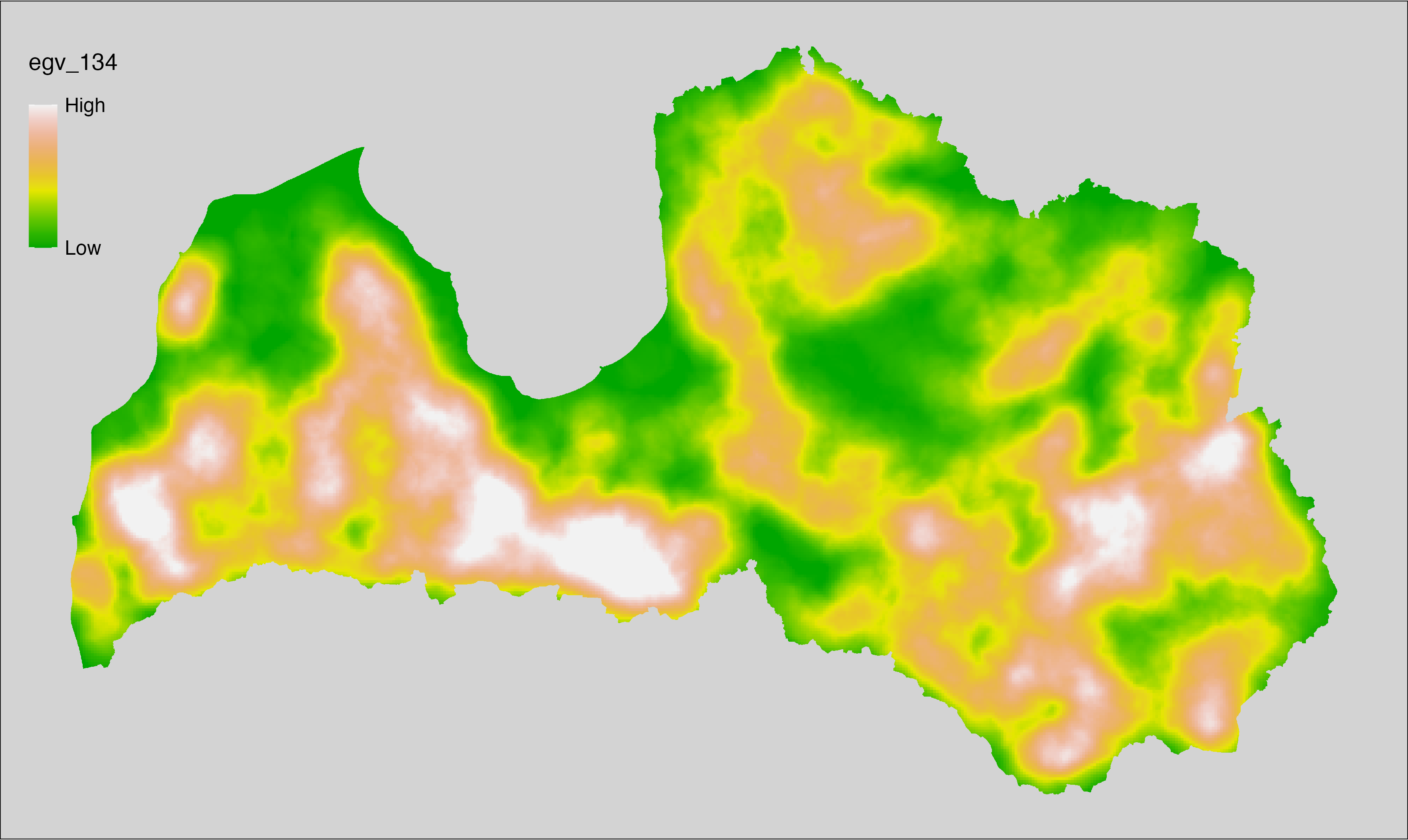
6.135 Edges_FarmlandShrubs-Trees_cell
filename: Edges_FarmlandShrubs-Trees_cell.tif
layername: egv_135
English name: Edge pixels of Farmland, Clear-Cuts, Shrubs bordering with Trees within the analysis cell (1 ha)
Latvian name: Lauksaimniecības zemju, izcirtumu, krūmu malu ar kokiem pikseļu skaits analīzes šūnā (1 ha)
Procedure: First, values between 300 and 400 and between 600 and 630 from
Landscape classification are coded as 0, and all other values as NA.
Then values larger than or equal to 630 but smaller than 700 from the Landscape
classification are coded as 1, and all other values as NA. Then, the
first layer (0 = presence) is covered over the second layer (presence = 1) and
written to file (matching the input). Next, using the workflow
egvtools::landscape_function() total edge between the two classes is
calculated. During the calculation of the landscape metric, inverse distance weighted
(power = 2) gap filling on the output is applied to ensure no missing values
at the edges. Finally, the layer is standardised by subtracting the arithmetic
mean and dividing by the root mean squared error.
Code
# libs ----
if(!require(terra)) {install.packages("terra"); require(terra)}
if(!require(egvtools)) {remotes::install_github("aavotins/egvtools"); require(egvtools)}
if(!require(sf)) {install.packages("sf"); require(sf)}
if(!require(sfarrow)) {install.packages("sfarrow"); require(sfarrow)}
if(!require(raster)) {install.packages("raster"); require(raster)}
if(!require(fasterize)) {install.packages("fasterize"); require(fasterize)}
if(!require(tidyverse)) {install.packages("tidyverse"); require(tidyverse)}
# Templates -----
template10=rast("./Templates/TemplateRasters/LV10m_10km.tif")
nulls10=rast("./Templates/TemplateRasters/nulls_LV10m_10km.tif")
# simple landscape ----
simple_landscape=rast("./RasterGrids_10m/2024/Ainava_vienk_mask.tif")
# Edges_FarmlandShrubs-Trees_input.tif ----
farmshrub=ifel((simple_landscape>300 & simple_landscape<400)|
(simple_landscape>600 & simple_landscape<630),0,NA)
trees_from630=ifel(simple_landscape>=630 & simple_landscape<700,1,NA)
plot(trees_from630)
farmshrub_trees630=cover(farmshrub,trees_from630)
plot(farmshrub_trees630)
edge_farmshrub_trees630=project(farmshrub_trees630,template10,
filename="./RasterGrids_10m/2024/Edges_FarmlandShrubs-Trees_input.tif",
overwrite=TRUE)
rm(edge_farmshrub_trees630)
rm(farmshrub_trees630)
# Edges_FarmlandShrubs-Trees_cell.tif egv_135 ----
landscape_function(
landscape = "./RasterGrids_10m/2024/Edges_FarmlandShrubs-Trees_input.tif",
zones = "./Templates/TemplateGrids/tikls100_sauzeme.parquet",
id_field = "id",
tile_field = "tks50km",
template = "./Templates/TemplateRasters/LV100m_10km.tif",
out_dir = "./RasterGrids_100m/2024/RAW",
out_filename = "Edges_FarmlandShrubs-Trees_cell.tif",
out_layername = "egv_135",
what = "lsm_l_te",
lm_args = list(count_boundary = FALSE),
rasterize_engine = "fasterize",
n_workers = 12,
future_max_size = 20 * 1024^3,
fill_gaps = TRUE,
plot_gaps = FALSE,
plot_result = FALSE
)
# standardisation ----
if(!require(terra)) {install.packages("terra"); require(terra)}
if(!require(tidyverse)) {install.packages("tidyverse"); require(tidyverse)}
nosaukums="Edges_FarmlandShrubs-Trees_cell.tif"
ielasisanas_cels=paste0("./RasterGrids_100m/2024/RAW/",nosaukums)
saglabasanas_cels=paste0("./RasterGrids_100m/2024/Scaled/",nosaukums)
slanis=rast(ielasisanas_cels)
videjais=global(slanis,fun="mean",na.rm=TRUE)
centrets=slanis-videjais[,1]
standartnovirze=terra::global(centrets,fun="rms",na.rm=TRUE)
merogots=centrets/standartnovirze[,1]
writeRaster(merogots,
filename=saglabasanas_cels,
overwrite=TRUE)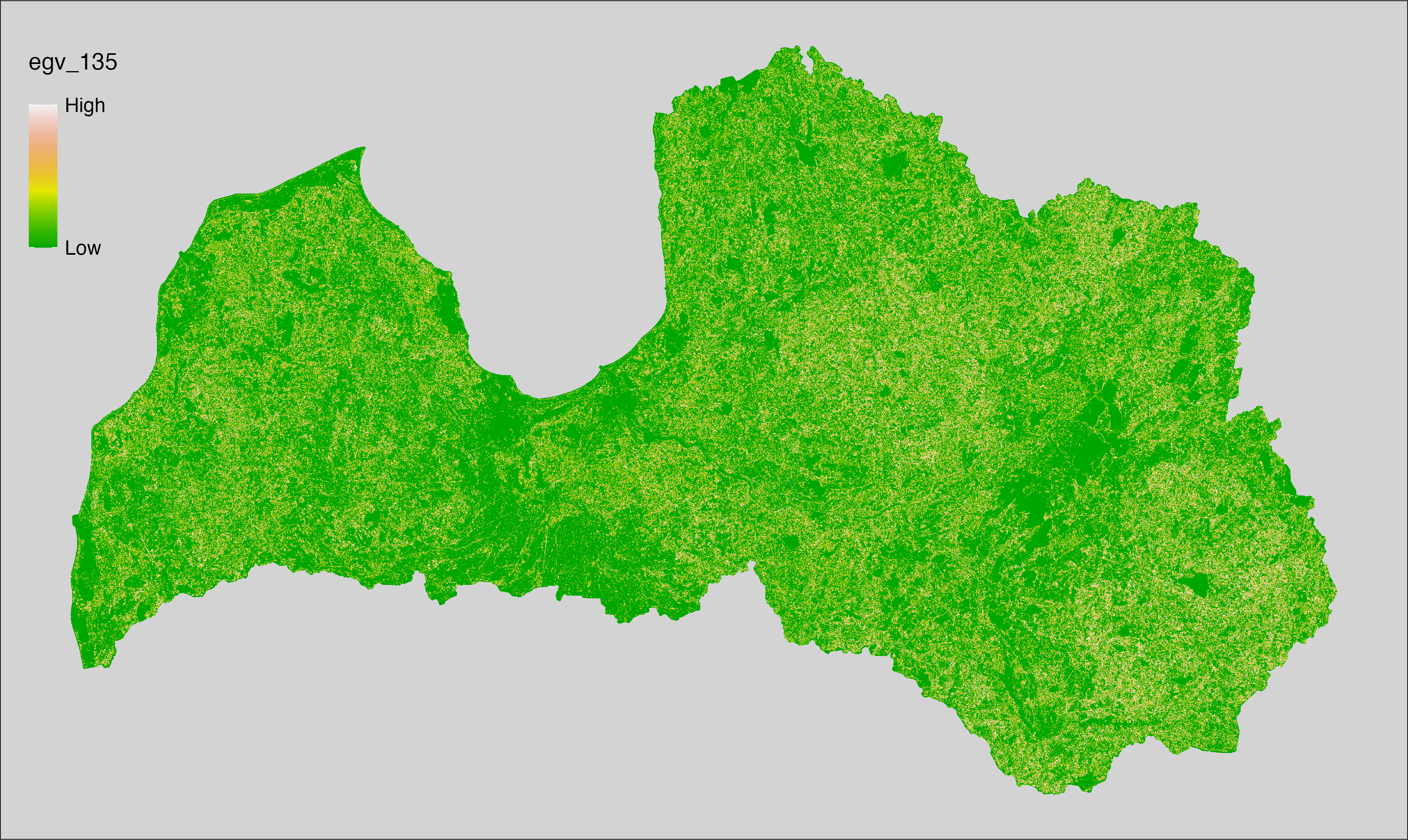
6.136 Edges_FarmlandShrubs-Trees_r500
filename: Edges_FarmlandShrubs-Trees_r500.tif
layername: egv_136
English name: Edge pixels of Farmland, Clear-Cuts, Shrubs bordering with Trees within the 0.5 km landscape
Latvian name: Lauksaimniecības zemju, izcirtumu, krūmu malu ar kokiem pikseļu skaits 0,5 km ainavā
Procedure: The total edge within a 500 m radius around the analysis grid cell is
calculated as the area-weighted sum of the analysis cells inside the
buffer, using the workflow egvtools::radius_function(). During the calculation of the landscape metric,
inverse distance weighted (power = 2) gap filling on the output is applied
to ensure no missing values at the edges. Then the layer is rewritten to set
its name. Finally, the layer is standardised by subtracting the arithmetic
mean and dividing by the root mean squared error.
Code
# libs ----
if(!require(terra)) {install.packages("terra"); require(terra)}
if(!require(egvtools)) {remotes::install_github("aavotins/egvtools"); require(egvtools)}
# Templates -----
template100=rast("./Templates/TemplateRasters/LV100m_10km.tif")
# radii ----
radius_function(
kvadrati_path = "./Templates/TemplateGrids/tiles/",
radii_path = "./Templates/TemplateGridPoints/tiles/",
tikls100_path = "./Templates/TemplateGrids/tikls100_sauzeme.parquet",
template_path = "./Templates/TemplateRasters/LV100m_10km.tif",
input_layers = c("./RasterGrids_100m/2024/RAW/Edges_FarmlandShrubs-Trees_cell.tif"),
layer_prefixes = c("Edges_FarmlandShrubs-Trees"),
output_dir = "./RasterGrids_100m/2024/RAW/",
n_workers = 12,
radii = c("r500"),
radius_mode = "sparse",
extract_fun = "sum",
fill_missing = TRUE,
IDW_weight = 2,
future_max_size = 20 * 1024^3)
# Edges_FarmlandShrubs-Trees_r500.tif egv_136 ----
slanis=rast("./RasterGrids_100m/2024/RAW/Edges_FarmlandShrubs-Trees_r500.tif")
names(slanis)="egv_136"
slanis2=project(slanis,template100)
writeRaster(slanis2,
"./RasterGrids_100m/2024/RAW/Edges_FarmlandShrubs-Trees_r500.tif",
overwrite=TRUE)
# standardisation ----
if(!require(terra)) {install.packages("terra"); require(terra)}
if(!require(tidyverse)) {install.packages("tidyverse"); require(tidyverse)}
nosaukums="Edges_FarmlandShrubs-Trees_r500.tif"
ielasisanas_cels=paste0("./RasterGrids_100m/2024/RAW/",nosaukums)
saglabasanas_cels=paste0("./RasterGrids_100m/2024/Scaled/",nosaukums)
slanis=rast(ielasisanas_cels)
videjais=global(slanis,fun="mean",na.rm=TRUE)
centrets=slanis-videjais[,1]
standartnovirze=terra::global(centrets,fun="rms",na.rm=TRUE)
merogots=centrets/standartnovirze[,1]
writeRaster(merogots,
filename=saglabasanas_cels,
overwrite=TRUE)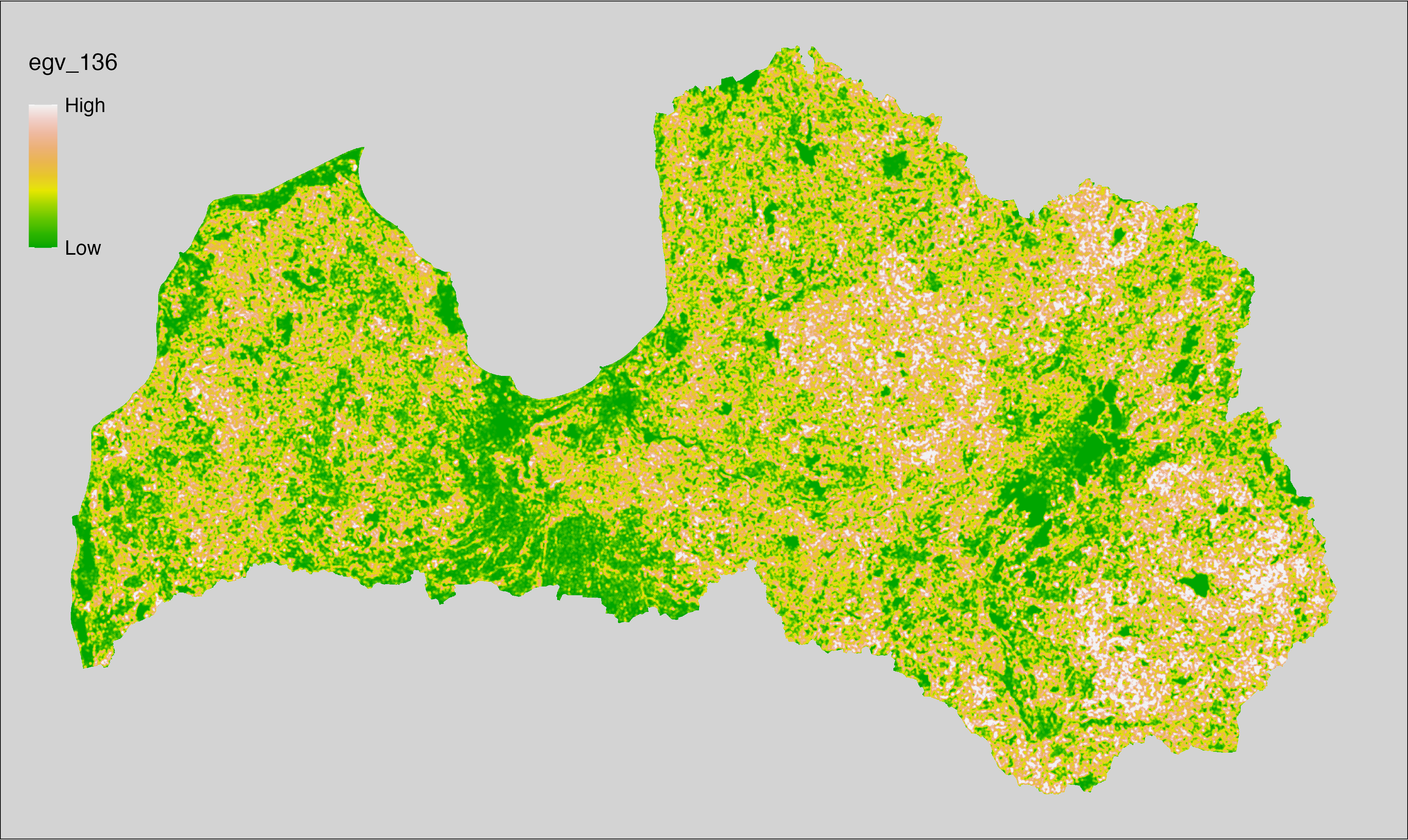
6.137 Edges_FarmlandShrubs-Trees_r1250
filename: Edges_FarmlandShrubs-Trees_r1250.tif
layername: egv_137
English name: Edge pixels of Farmland, Clear-Cuts, Shrubs bordering with Trees within the 1.25 km landscape
Latvian name: Lauksaimniecības zemju, izcirtumu, krūmu malu ar kokiem pikseļu skaits 1,25 km ainavā
Procedure: The total edge within a 1250 m radius around the analysis grid cell is
calculated as the area-weighted sum of the analysis cells inside the
buffer, using the workflow egvtools::radius_function(). During the calculation of the landscape metric,
inverse distance weighted (power = 2) gap filling on the output is applied
to ensure no missing values at the edges. Then the layer is rewritten to set
its name. Finally, the layer is standardised by subtracting the arithmetic
mean and dividing by the root mean squared error.
Code
# libs ----
if(!require(terra)) {install.packages("terra"); require(terra)}
if(!require(egvtools)) {remotes::install_github("aavotins/egvtools"); require(egvtools)}
# Templates -----
template100=rast("./Templates/TemplateRasters/LV100m_10km.tif")
# radii ----
radius_function(
kvadrati_path = "./Templates/TemplateGrids/tiles/",
radii_path = "./Templates/TemplateGridPoints/tiles/",
tikls100_path = "./Templates/TemplateGrids/tikls100_sauzeme.parquet",
template_path = "./Templates/TemplateRasters/LV100m_10km.tif",
input_layers = c("./RasterGrids_100m/2024/RAW/Edges_FarmlandShrubs-Trees_cell.tif"),
layer_prefixes = c("Edges_FarmlandShrubs-Trees"),
output_dir = "./RasterGrids_100m/2024/RAW/",
n_workers = 12,
radii = c("r1250"),
radius_mode = "sparse",
extract_fun = "sum",
fill_missing = TRUE,
IDW_weight = 2,
future_max_size = 20 * 1024^3)
# Edges_FarmlandShrubs-Trees_r1250.tif egv_137 ----
slanis=rast("./RasterGrids_100m/2024/RAW/Edges_FarmlandShrubs-Trees_r1250.tif")
names(slanis)="egv_137"
slanis2=project(slanis,template100)
writeRaster(slanis2,
"./RasterGrids_100m/2024/RAW/Edges_FarmlandShrubs-Trees_r1250.tif",
overwrite=TRUE)
# standardisation ----
if(!require(terra)) {install.packages("terra"); require(terra)}
if(!require(tidyverse)) {install.packages("tidyverse"); require(tidyverse)}
nosaukums="Edges_FarmlandShrubs-Trees_r1250.tif"
ielasisanas_cels=paste0("./RasterGrids_100m/2024/RAW/",nosaukums)
saglabasanas_cels=paste0("./RasterGrids_100m/2024/Scaled/",nosaukums)
slanis=rast(ielasisanas_cels)
videjais=global(slanis,fun="mean",na.rm=TRUE)
centrets=slanis-videjais[,1]
standartnovirze=terra::global(centrets,fun="rms",na.rm=TRUE)
merogots=centrets/standartnovirze[,1]
writeRaster(merogots,
filename=saglabasanas_cels,
overwrite=TRUE)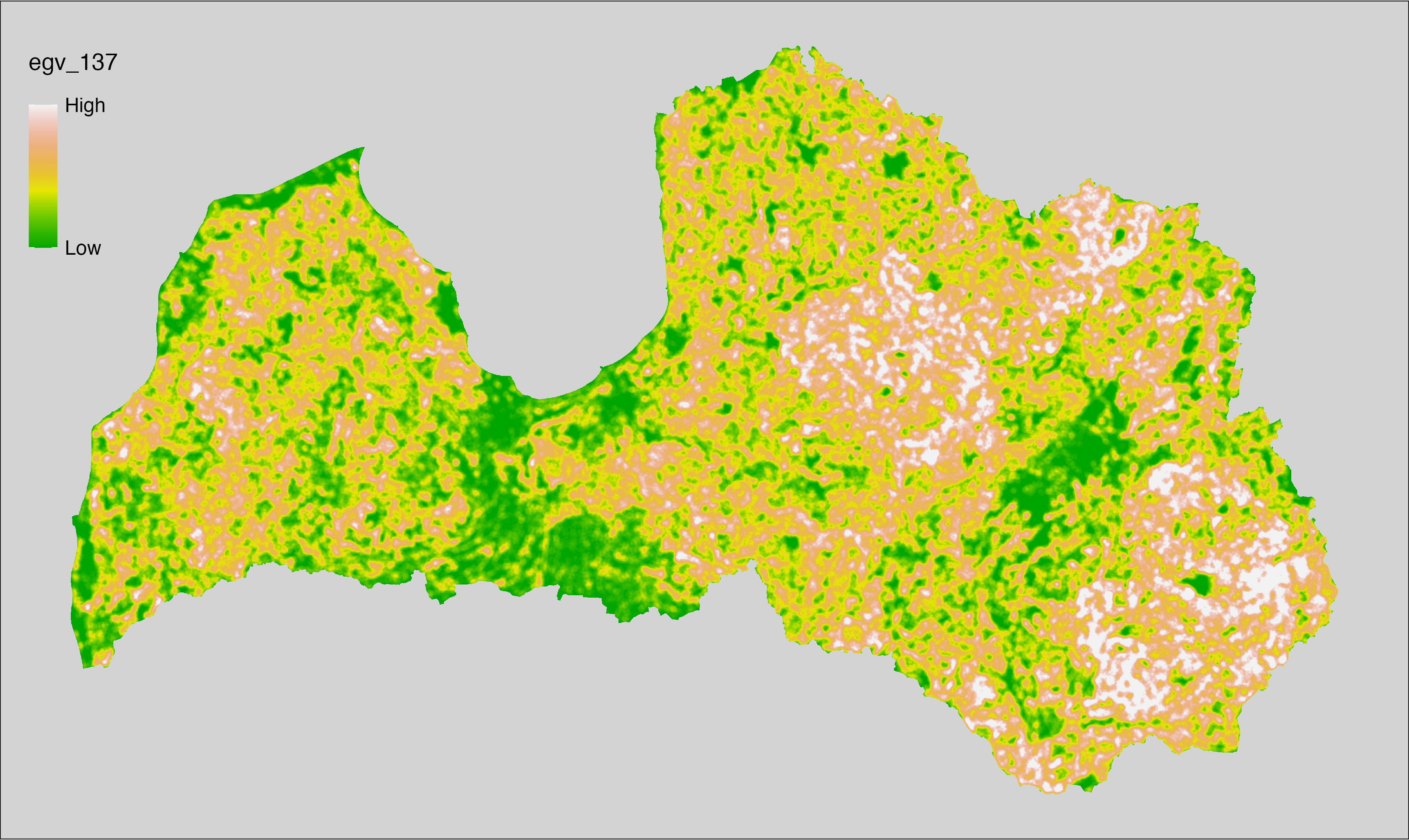
6.138 Edges_FarmlandShrubs-Trees_r3000
filename: Edges_FarmlandShrubs-Trees_r3000.tif
layername: egv_138
English name: Edge pixels of Farmland, Clear-Cuts, Shrubs bordering with Trees within the 3 km landscape
Latvian name: Lauksaimniecības zemju, izcirtumu, krūmu malu ar kokiem pikseļu skaits 3 km ainavā
Procedure: The total edge within a 3000 m radius around the analysis grid cell is
calculated as the area-weighted sum of the analysis cells inside the
buffer, using the workflow egvtools::radius_function(). During the calculation of the landscape metric,
inverse distance weighted (power = 2) gap filling on the output is applied
to ensure no missing values at the edges. Then the layer is rewritten to set
its name. Finally, the layer is standardised by subtracting the arithmetic
mean and dividing by the root mean squared error.
Code
# libs ----
if(!require(terra)) {install.packages("terra"); require(terra)}
if(!require(egvtools)) {remotes::install_github("aavotins/egvtools"); require(egvtools)}
# Templates -----
template100=rast("./Templates/TemplateRasters/LV100m_10km.tif")
# radii ----
radius_function(
kvadrati_path = "./Templates/TemplateGrids/tiles/",
radii_path = "./Templates/TemplateGridPoints/tiles/",
tikls100_path = "./Templates/TemplateGrids/tikls100_sauzeme.parquet",
template_path = "./Templates/TemplateRasters/LV100m_10km.tif",
input_layers = c("./RasterGrids_100m/2024/RAW/Edges_FarmlandShrubs-Trees_cell.tif"),
layer_prefixes = c("Edges_FarmlandShrubs-Trees"),
output_dir = "./RasterGrids_100m/2024/RAW/",
n_workers = 12,
radii = c("r3000"),
radius_mode = "sparse",
extract_fun = "sum",
fill_missing = TRUE,
IDW_weight = 2,
future_max_size = 20 * 1024^3)
# Edges_FarmlandShrubs-Trees_r3000.tif egv_138 ----
slanis=rast("./RasterGrids_100m/2024/RAW/Edges_FarmlandShrubs-Trees_r3000.tif")
names(slanis)="egv_138"
slanis2=project(slanis,template100)
writeRaster(slanis2,
"./RasterGrids_100m/2024/RAW/Edges_FarmlandShrubs-Trees_r3000.tif",
overwrite=TRUE)
# standardisation ----
if(!require(terra)) {install.packages("terra"); require(terra)}
if(!require(tidyverse)) {install.packages("tidyverse"); require(tidyverse)}
nosaukums="Edges_FarmlandShrubs-Trees_r3000.tif"
ielasisanas_cels=paste0("./RasterGrids_100m/2024/RAW/",nosaukums)
saglabasanas_cels=paste0("./RasterGrids_100m/2024/Scaled/",nosaukums)
slanis=rast(ielasisanas_cels)
videjais=global(slanis,fun="mean",na.rm=TRUE)
centrets=slanis-videjais[,1]
standartnovirze=terra::global(centrets,fun="rms",na.rm=TRUE)
merogots=centrets/standartnovirze[,1]
writeRaster(merogots,
filename=saglabasanas_cels,
overwrite=TRUE)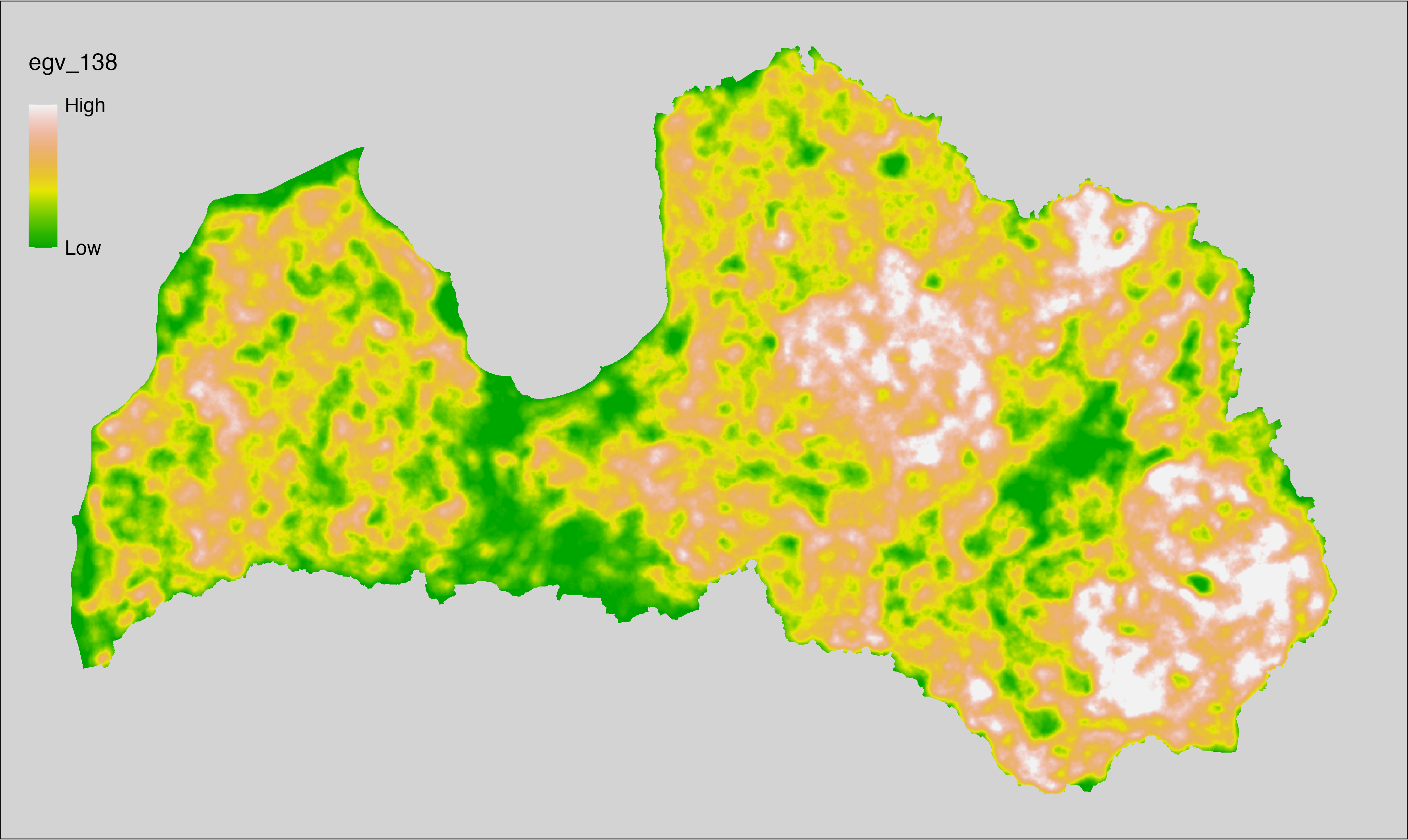
6.139 Edges_FarmlandShrubs-Trees_r10000
filename: Edges_FarmlandShrubs-Trees_r10000.tif
layername: egv_139
English name: Edge pixels of Farmland, Clear-Cuts, Shrubs bordering with Trees within the 10 km landscape
Latvian name: Lauksaimniecības zemju, izcirtumu, krūmu malu ar kokiem pikseļu skaits 10 km ainavā
Procedure: The total edge within a 10000 m radius around the analysis grid cell is
calculated as the area-weighted sum of the analysis cells inside the
buffer, using the workflow egvtools::radius_function(). During the calculation of the landscape metric,
inverse distance weighted (power = 2) gap filling on the output is applied
to ensure no missing values at the edges. Then the layer is rewritten to set
its name. Finally, the layer is standardised by subtracting the arithmetic
mean and dividing by the root mean squared error.
Code
# libs ----
if(!require(terra)) {install.packages("terra"); require(terra)}
if(!require(egvtools)) {remotes::install_github("aavotins/egvtools"); require(egvtools)}
# Templates -----
template100=rast("./Templates/TemplateRasters/LV100m_10km.tif")
# radii ----
radius_function(
kvadrati_path = "./Templates/TemplateGrids/tiles/",
radii_path = "./Templates/TemplateGridPoints/tiles/",
tikls100_path = "./Templates/TemplateGrids/tikls100_sauzeme.parquet",
template_path = "./Templates/TemplateRasters/LV100m_10km.tif",
input_layers = c("./RasterGrids_100m/2024/RAW/Edges_FarmlandShrubs-Trees_cell.tif"),
layer_prefixes = c("Edges_FarmlandShrubs-Trees"),
output_dir = "./RasterGrids_100m/2024/RAW/",
n_workers = 12,
radii = c("r10000"),
radius_mode = "sparse",
extract_fun = "sum",
fill_missing = TRUE,
IDW_weight = 2,
future_max_size = 20 * 1024^3)
# Edges_FarmlandShrubs-Trees_r10000.tif egv_139 ----
slanis=rast("./RasterGrids_100m/2024/RAW/Edges_FarmlandShrubs-Trees_r10000.tif")
names(slanis)="egv_139"
slanis2=project(slanis,template100)
writeRaster(slanis2,
"./RasterGrids_100m/2024/RAW/Edges_FarmlandShrubs-Trees_r10000.tif",
overwrite=TRUE)
# standardisation ----
if(!require(terra)) {install.packages("terra"); require(terra)}
if(!require(tidyverse)) {install.packages("tidyverse"); require(tidyverse)}
nosaukums="Edges_FarmlandShrubs-Trees_r10000.tif"
ielasisanas_cels=paste0("./RasterGrids_100m/2024/RAW/",nosaukums)
saglabasanas_cels=paste0("./RasterGrids_100m/2024/Scaled/",nosaukums)
slanis=rast(ielasisanas_cels)
videjais=global(slanis,fun="mean",na.rm=TRUE)
centrets=slanis-videjais[,1]
standartnovirze=terra::global(centrets,fun="rms",na.rm=TRUE)
merogots=centrets/standartnovirze[,1]
writeRaster(merogots,
filename=saglabasanas_cels,
overwrite=TRUE)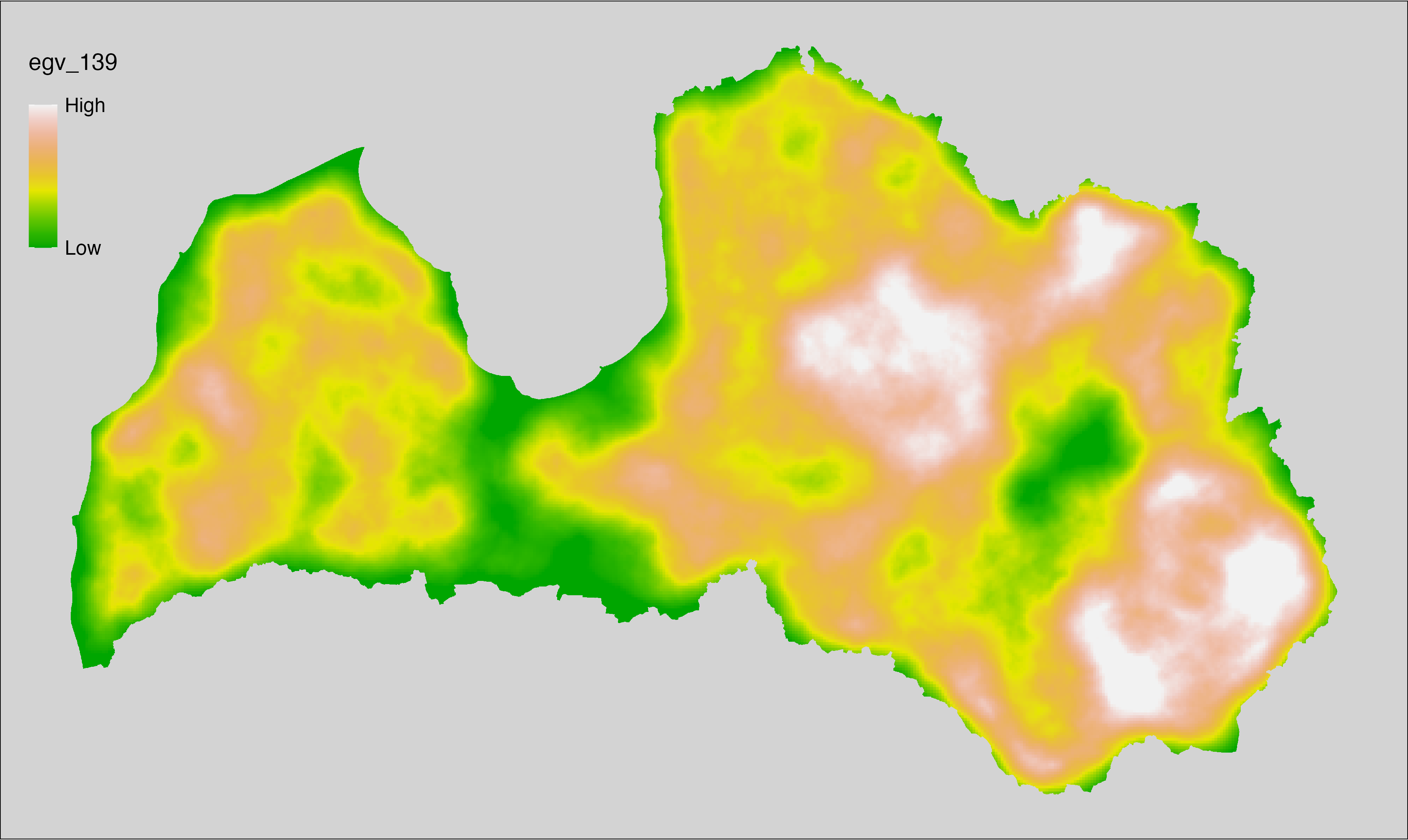
6.140 Edges_Grasslands_cell
filename: Edges_Grasslands_cell.tif
layername: egv_140
English name: Edge pixels of Grassland within the analysis cell (1 ha)
Latvian name: Zālāju malu pikseļu skaits analīzes šūnā (1 ha)
Procedure: First, values equal to 330 from the Landscape
classification are coded as 1, and all other values as NA. Then, the
layer (1 = presence) is covered over the nulls layer (presence = 0) and written to
file (matching the input). Then, using the workflow
egvtools::landscape_function() total edge between the two classes is
calculated. During the calculation of the landscape metric, inverse distance weighted
(power = 2) gap filling on the output is applied to ensure no missing values
at the edges. Finally, the layer is standardised by subtracting the arithmetic
mean and dividing by the root mean squared error.
Code
# libs ----
if(!require(terra)) {install.packages("terra"); require(terra)}
if(!require(egvtools)) {remotes::install_github("aavotins/egvtools"); require(egvtools)}
if(!require(sf)) {install.packages("sf"); require(sf)}
if(!require(sfarrow)) {install.packages("sfarrow"); require(sfarrow)}
if(!require(raster)) {install.packages("raster"); require(raster)}
if(!require(fasterize)) {install.packages("fasterize"); require(fasterize)}
if(!require(tidyverse)) {install.packages("tidyverse"); require(tidyverse)}
# Templates -----
template10=rast("./Templates/TemplateRasters/LV10m_10km.tif")
nulls10=rast("./Templates/TemplateRasters/nulls_LV10m_10km.tif")
# simple landscape ----
simple_landscape=rast("./RasterGrids_10m/2024/Ainava_vienk_mask.tif")
# Edges_Grasslands_input.tif ----
grassland=ifel(simple_landscape==330,1,NA)
plot(grassland)
grassland=cover(grassland,nulls10)
plot(grassland)
edge_grassland=project(grassland,template10,
filename="./RasterGrids_10m/2024/Edges_Grasslands_input.tif",
overwrite=TRUE)
rm(edge_grassland)
# Edges_Grasslands_cell.tif egv_140 ----
landscape_function(
landscape = "./RasterGrids_10m/2024/Edges_Grasslands_input.tif",
zones = "./Templates/TemplateGrids/tikls100_sauzeme.parquet",
id_field = "id",
tile_field = "tks50km",
template = "./Templates/TemplateRasters/LV100m_10km.tif",
out_dir = "./RasterGrids_100m/2024/RAW",
out_filename = "Edges_Grasslands_cell.tif",
out_layername = "egv_140",
what = "lsm_l_te",
lm_args = list(count_boundary = FALSE),
rasterize_engine = "fasterize",
n_workers = 12,
future_max_size = 20 * 1024^3,
fill_gaps = TRUE,
plot_gaps = FALSE,
plot_result = FALSE
)
# standardisation ----
if(!require(terra)) {install.packages("terra"); require(terra)}
if(!require(tidyverse)) {install.packages("tidyverse"); require(tidyverse)}
nosaukums="Edges_Grasslands_cell.tif"
ielasisanas_cels=paste0("./RasterGrids_100m/2024/RAW/",nosaukums)
saglabasanas_cels=paste0("./RasterGrids_100m/2024/Scaled/",nosaukums)
slanis=rast(ielasisanas_cels)
videjais=global(slanis,fun="mean",na.rm=TRUE)
centrets=slanis-videjais[,1]
standartnovirze=terra::global(centrets,fun="rms",na.rm=TRUE)
merogots=centrets/standartnovirze[,1]
writeRaster(merogots,
filename=saglabasanas_cels,
overwrite=TRUE)
6.141 Edges_Grasslands_r500
filename: Edges_Grasslands_r500.tif
layername: egv_141
English name: Edge pixels of Grassland within the 0.5 km landscape
Latvian name: Zālāju malu pikseļu skaits 0,5 km ainavā
Procedure: The total edge within a 500 m radius around the analysis grid cell is
calculated as the area-weighted sum of the analysis cells inside the
buffer, using the workflow egvtools::radius_function(). During the calculation of the landscape metric,
inverse distance weighted (power = 2) gap filling on the output is applied
to ensure no missing values at the edges. Then the layer is rewritten to set
its name. Finally, the layer is standardised by subtracting the arithmetic
mean and dividing by the root mean squared error.
Code
# libs ----
if(!require(terra)) {install.packages("terra"); require(terra)}
if(!require(egvtools)) {remotes::install_github("aavotins/egvtools"); require(egvtools)}
# Templates -----
template100=rast("./Templates/TemplateRasters/LV100m_10km.tif")
# radii ----
radius_function(
kvadrati_path = "./Templates/TemplateGrids/tiles/",
radii_path = "./Templates/TemplateGridPoints/tiles/",
tikls100_path = "./Templates/TemplateGrids/tikls100_sauzeme.parquet",
template_path = "./Templates/TemplateRasters/LV100m_10km.tif",
input_layers = c("./RasterGrids_100m/2024/RAW/Edges_Grasslands_cell.tif"),
layer_prefixes = c("Edges_Grasslands"),
output_dir = "./RasterGrids_100m/2024/RAW/",
n_workers = 12,
radii = c("r500"),
radius_mode = "sparse",
extract_fun = "sum",
fill_missing = TRUE,
IDW_weight = 2,
future_max_size = 20 * 1024^3)
# Edges_Grasslands_r500.tif egv_141 ----
slanis=rast("./RasterGrids_100m/2024/RAW/Edges_Grasslands_r500.tif")
names(slanis)="egv_141"
slanis2=project(slanis,template100)
writeRaster(slanis2,
"./RasterGrids_100m/2024/RAW/Edges_Grasslands_r500.tif",
overwrite=TRUE)
# standardisation ----
if(!require(terra)) {install.packages("terra"); require(terra)}
if(!require(tidyverse)) {install.packages("tidyverse"); require(tidyverse)}
nosaukums="Edges_Grasslands_r500.tif"
ielasisanas_cels=paste0("./RasterGrids_100m/2024/RAW/",nosaukums)
saglabasanas_cels=paste0("./RasterGrids_100m/2024/Scaled/",nosaukums)
slanis=rast(ielasisanas_cels)
videjais=global(slanis,fun="mean",na.rm=TRUE)
centrets=slanis-videjais[,1]
standartnovirze=terra::global(centrets,fun="rms",na.rm=TRUE)
merogots=centrets/standartnovirze[,1]
writeRaster(merogots,
filename=saglabasanas_cels,
overwrite=TRUE)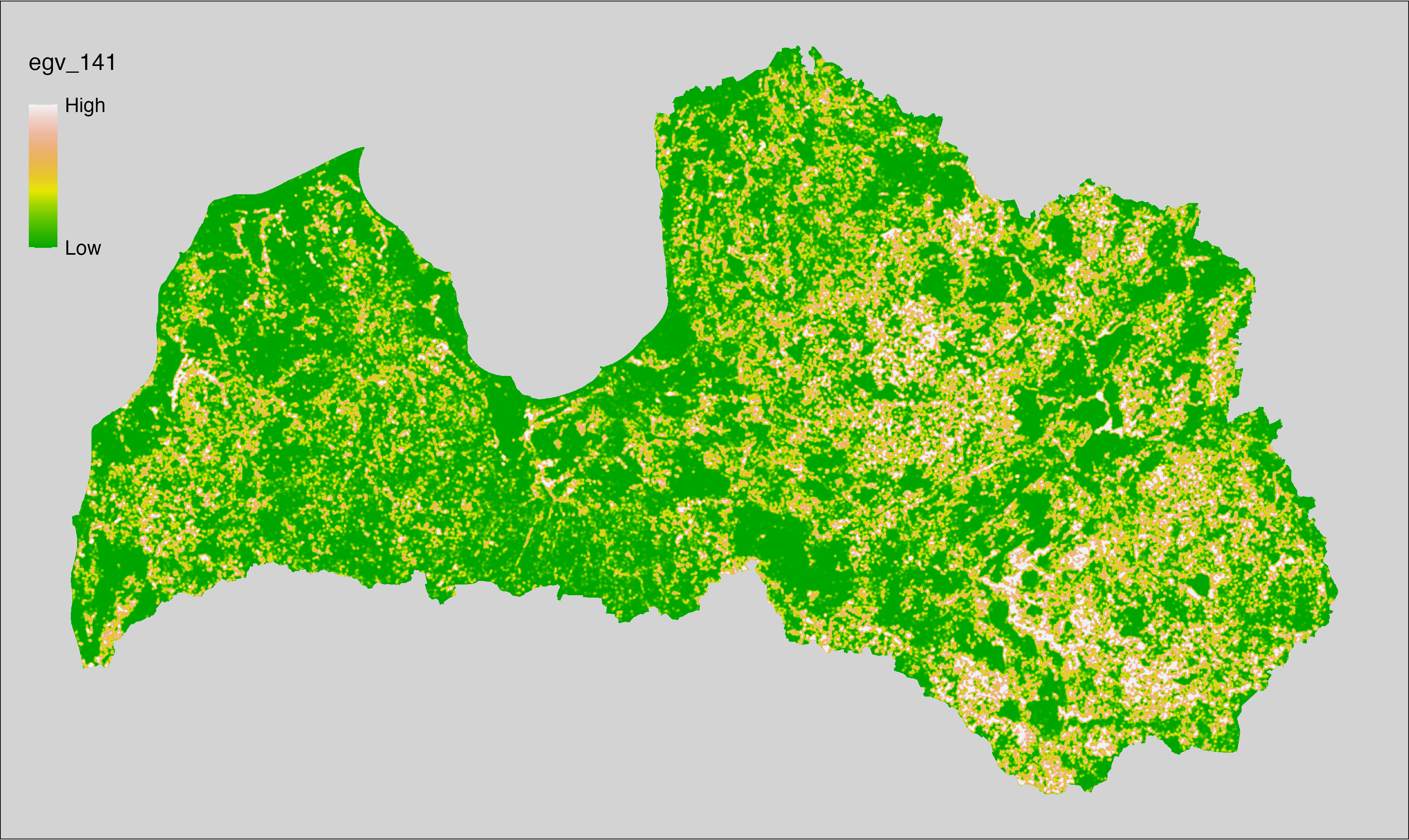
6.142 Edges_Grasslands_r1250
filename: Edges_Grasslands_r1250.tif
layername: egv_142
English name: Edge pixels of Grassland within the 1.25 km landscape
Latvian name: Zālāju malu pikseļu skaits 1,25 km ainavā
Procedure: The total edge within a 1250 m radius around the analysis grid cell is
calculated as the area-weighted sum of the analysis cells inside the
buffer, using the workflow egvtools::radius_function(). During the calculation of the landscape metric,
inverse distance weighted (power = 2) gap filling on the output is applied
to ensure no missing values at the edges. Then the layer is rewritten to set
its name. Finally, the layer is standardised by subtracting the arithmetic
mean and dividing by the root mean squared error.
Code
# libs ----
if(!require(terra)) {install.packages("terra"); require(terra)}
if(!require(egvtools)) {remotes::install_github("aavotins/egvtools"); require(egvtools)}
# Templates -----
template100=rast("./Templates/TemplateRasters/LV100m_10km.tif")
# radii ----
radius_function(
kvadrati_path = "./Templates/TemplateGrids/tiles/",
radii_path = "./Templates/TemplateGridPoints/tiles/",
tikls100_path = "./Templates/TemplateGrids/tikls100_sauzeme.parquet",
template_path = "./Templates/TemplateRasters/LV100m_10km.tif",
input_layers = c("./RasterGrids_100m/2024/RAW/Edges_Grasslands_cell.tif"),
layer_prefixes = c("Edges_Grasslands"),
output_dir = "./RasterGrids_100m/2024/RAW/",
n_workers = 12,
radii = c("r1250"),
radius_mode = "sparse",
extract_fun = "sum",
fill_missing = TRUE,
IDW_weight = 2,
future_max_size = 20 * 1024^3)
# Edges_Grasslands_r1250.tif egv_142 ----
slanis=rast("./RasterGrids_100m/2024/RAW/Edges_Grasslands_r1250.tif")
names(slanis)="egv_142"
slanis2=project(slanis,template100)
writeRaster(slanis2,
"./RasterGrids_100m/2024/RAW/Edges_Grasslands_r1250.tif",
overwrite=TRUE)
# standardisation ----
if(!require(terra)) {install.packages("terra"); require(terra)}
if(!require(tidyverse)) {install.packages("tidyverse"); require(tidyverse)}
nosaukums="Edges_Grasslands_r1250.tif"
ielasisanas_cels=paste0("./RasterGrids_100m/2024/RAW/",nosaukums)
saglabasanas_cels=paste0("./RasterGrids_100m/2024/Scaled/",nosaukums)
slanis=rast(ielasisanas_cels)
videjais=global(slanis,fun="mean",na.rm=TRUE)
centrets=slanis-videjais[,1]
standartnovirze=terra::global(centrets,fun="rms",na.rm=TRUE)
merogots=centrets/standartnovirze[,1]
writeRaster(merogots,
filename=saglabasanas_cels,
overwrite=TRUE)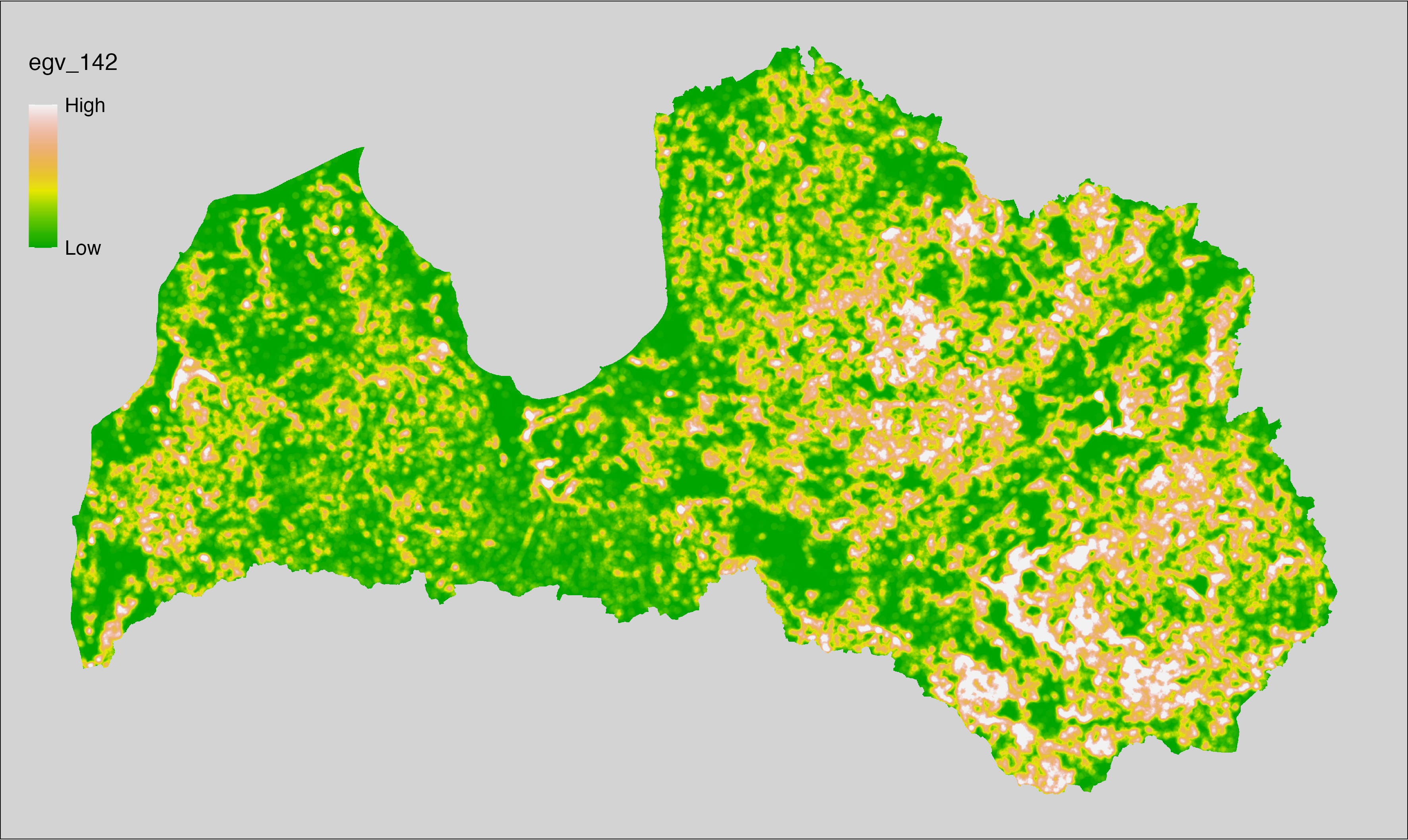
6.143 Edges_Grasslands_r3000
filename: Edges_Grasslands_r3000.tif
layername: egv_143
English name: Edge pixels of Grassland within the 3 km landscape
Latvian name: Zālāju malu pikseļu skaits 3 km ainavā
Procedure: The total edge within a 3000 m radius around the analysis grid cell is
calculated as the area-weighted sum of the analysis cells inside the
buffer, using the workflow egvtools::radius_function(). During the calculation of the landscape metric,
inverse distance weighted (power = 2) gap filling on the output is applied
to ensure no missing values at the edges. Then the layer is rewritten to set
its name. Finally, the layer is standardised by subtracting the arithmetic
mean and dividing by the root mean squared error.
Code
# libs ----
if(!require(terra)) {install.packages("terra"); require(terra)}
if(!require(egvtools)) {remotes::install_github("aavotins/egvtools"); require(egvtools)}
# Templates -----
template100=rast("./Templates/TemplateRasters/LV100m_10km.tif")
# radii ----
radius_function(
kvadrati_path = "./Templates/TemplateGrids/tiles/",
radii_path = "./Templates/TemplateGridPoints/tiles/",
tikls100_path = "./Templates/TemplateGrids/tikls100_sauzeme.parquet",
template_path = "./Templates/TemplateRasters/LV100m_10km.tif",
input_layers = c("./RasterGrids_100m/2024/RAW/Edges_Grasslands_cell.tif"),
layer_prefixes = c("Edges_Grasslands"),
output_dir = "./RasterGrids_100m/2024/RAW/",
n_workers = 12,
radii = c("r3000"),
radius_mode = "sparse",
extract_fun = "sum",
fill_missing = TRUE,
IDW_weight = 2,
future_max_size = 20 * 1024^3)
# Edges_Grasslands_r3000.tif egv_143 ----
slanis=rast("./RasterGrids_100m/2024/RAW/Edges_Grasslands_r3000.tif")
names(slanis)="egv_143"
slanis2=project(slanis,template100)
writeRaster(slanis2,
"./RasterGrids_100m/2024/RAW/Edges_Grasslands_r3000.tif",
overwrite=TRUE)
# standardisation ----
if(!require(terra)) {install.packages("terra"); require(terra)}
if(!require(tidyverse)) {install.packages("tidyverse"); require(tidyverse)}
nosaukums="Edges_Grasslands_r3000.tif"
ielasisanas_cels=paste0("./RasterGrids_100m/2024/RAW/",nosaukums)
saglabasanas_cels=paste0("./RasterGrids_100m/2024/Scaled/",nosaukums)
slanis=rast(ielasisanas_cels)
videjais=global(slanis,fun="mean",na.rm=TRUE)
centrets=slanis-videjais[,1]
standartnovirze=terra::global(centrets,fun="rms",na.rm=TRUE)
merogots=centrets/standartnovirze[,1]
writeRaster(merogots,
filename=saglabasanas_cels,
overwrite=TRUE)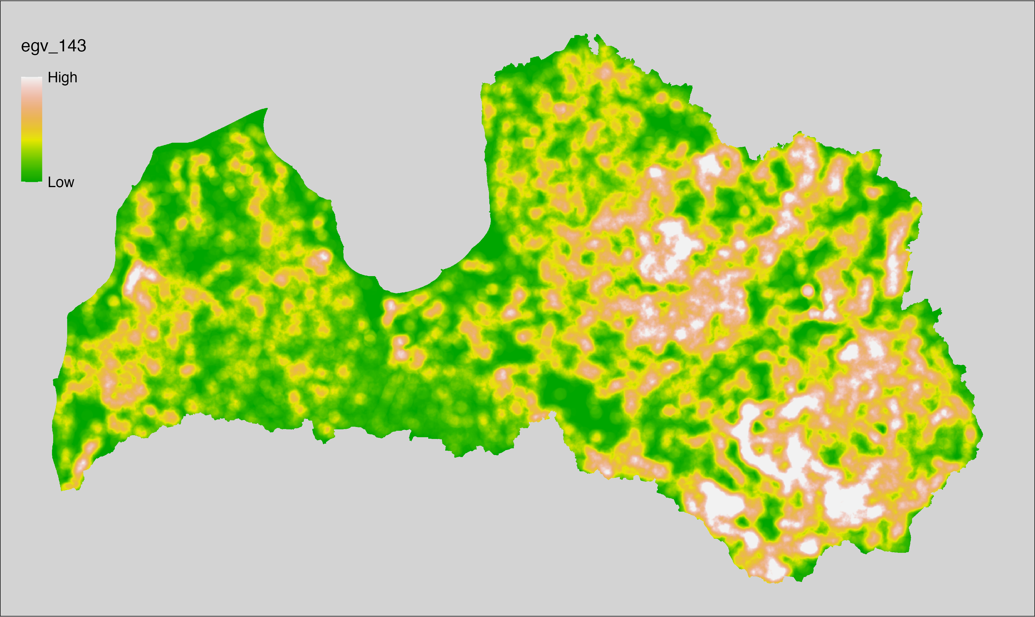
6.144 Edges_Grasslands_r10000
filename: Edges_Grasslands_r10000.tif
layername: egv_144
English name: Edge pixels of Grassland within the 10 km landscape
Latvian name: Zālāju malu pikseļu skaits 10 km ainavā
Procedure: The total edge within a 10000 m radius around the analysis grid cell is
calculated as the area-weighted sum of the analysis cells inside the
buffer, using the workflow egvtools::radius_function(). During the calculation of the landscape metric,
inverse distance weighted (power = 2) gap filling on the output is applied
to ensure no missing values at the edges. Then the layer is rewritten to set
its name. Finally, the layer is standardised by subtracting the arithmetic
mean and dividing by the root mean squared error.
Code
# libs ----
if(!require(terra)) {install.packages("terra"); require(terra)}
if(!require(egvtools)) {remotes::install_github("aavotins/egvtools"); require(egvtools)}
# Templates -----
template100=rast("./Templates/TemplateRasters/LV100m_10km.tif")
# radii ----
radius_function(
kvadrati_path = "./Templates/TemplateGrids/tiles/",
radii_path = "./Templates/TemplateGridPoints/tiles/",
tikls100_path = "./Templates/TemplateGrids/tikls100_sauzeme.parquet",
template_path = "./Templates/TemplateRasters/LV100m_10km.tif",
input_layers = c("./RasterGrids_100m/2024/RAW/Edges_Grasslands_cell.tif"),
layer_prefixes = c("Edges_Grasslands"),
output_dir = "./RasterGrids_100m/2024/RAW/",
n_workers = 12,
radii = c("r10000"),
radius_mode = "sparse",
extract_fun = "sum",
fill_missing = TRUE,
IDW_weight = 2,
future_max_size = 20 * 1024^3)
# Edges_Grasslands_r10000.tif egv_144 ----
slanis=rast("./RasterGrids_100m/2024/RAW/Edges_Grasslands_r10000.tif")
names(slanis)="egv_144"
slanis2=project(slanis,template100)
writeRaster(slanis2,
"./RasterGrids_100m/2024/RAW/Edges_Grasslands_r10000.tif",
overwrite=TRUE)
# standardisation ----
if(!require(terra)) {install.packages("terra"); require(terra)}
if(!require(tidyverse)) {install.packages("tidyverse"); require(tidyverse)}
nosaukums="Edges_Grasslands_r10000.tif"
ielasisanas_cels=paste0("./RasterGrids_100m/2024/RAW/",nosaukums)
saglabasanas_cels=paste0("./RasterGrids_100m/2024/Scaled/",nosaukums)
slanis=rast(ielasisanas_cels)
videjais=global(slanis,fun="mean",na.rm=TRUE)
centrets=slanis-videjais[,1]
standartnovirze=terra::global(centrets,fun="rms",na.rm=TRUE)
merogots=centrets/standartnovirze[,1]
writeRaster(merogots,
filename=saglabasanas_cels,
overwrite=TRUE)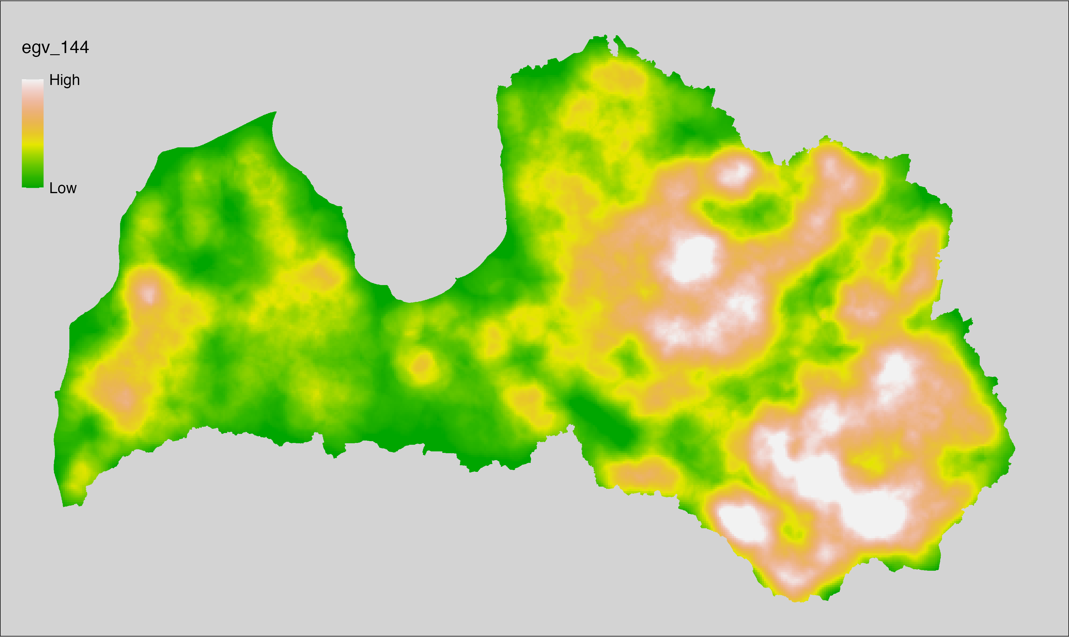
6.145 Edges_OldForests_cell
filename: Edges_OldForests_cell.tif
layername: egv_145
English name: Edge pixels of Forests Over Rotation Age within the analysis cell (1 ha)
Latvian name: Pieaugušo un pāraugušo mežaudžu malu pikseļu skaits analīzes šūnā (1 ha)
Procedure: First, the raster layer with forest stands from the MVR at
age groups 4 and 5 is prepared (presence = 1, everything else = NA). Then, the
layer (1 = presence) is covered over the nulls layer (presence = 0) and written to
file (matching the input). Then, using the workflow
egvtools::landscape_function() total edge between the two classes is
calculated. During the calculation of the landscape metric, inverse distance weighted
(power = 2) gap filling on the output is applied to ensure no missing values
at the edges. Finally, the layer is standardised by subtracting the arithmetic
mean and dividing by the root mean squared error.
Code
# libs ----
if(!require(terra)) {install.packages("terra"); require(terra)}
if(!require(egvtools)) {remotes::install_github("aavotins/egvtools"); require(egvtools)}
if(!require(sf)) {install.packages("sf"); require(sf)}
if(!require(sfarrow)) {install.packages("sfarrow"); require(sfarrow)}
if(!require(raster)) {install.packages("raster"); require(raster)}
if(!require(fasterize)) {install.packages("fasterize"); require(fasterize)}
if(!require(tidyverse)) {install.packages("tidyverse"); require(tidyverse)}
# Templates -----
template10=rast("./Templates/TemplateRasters/LV10m_10km.tif")
nulls10=rast("./Templates/TemplateRasters/nulls_LV10m_10km.tif")
# simple landscape ----
simple_landscape=rast("./RasterGrids_10m/2024/Ainava_vienk_mask.tif")
# Edges_OldForests_input.tif ----
mvr=sfarrow::st_read_parquet("./Geodata/2024/MVR/nogabali_2024janv.parquet")
mvr2=mvr %>%
mutate(forest_age=ifelse(vgr=="4"|vgr=="5",1,NA)) %>%
filter(!is.na(forest_age))
rast_old=fasterize(mvr2,raster(template10),field="forest_age")
terra_old=rast(rast_old)
plot(terra_old)
terra_old=cover(terra_old,nulls10)
plot(terra_old)
edge_old=project(terra_old,template10,
filename="./RasterGrids_10m/2024/Edges_OldForests_input.tif",
overwrite=TRUE)
rm(mvr)
rm(mvr2)
rm(rast_old)
rm(terra_old)
rm(edge_old)
# Edges_OldForests_cell.tif egv_145 ----
landscape_function(
landscape = "./RasterGrids_10m/2024/Edges_OldForests_input.tif",
zones = "./Templates/TemplateGrids/tikls100_sauzeme.parquet",
id_field = "id",
tile_field = "tks50km",
template = "./Templates/TemplateRasters/LV100m_10km.tif",
out_dir = "./RasterGrids_100m/2024/RAW",
out_filename = "Edges_OldForests_cell.tif",
out_layername = "egv_145",
what = "lsm_l_te",
lm_args = list(count_boundary = FALSE),
rasterize_engine = "fasterize",
n_workers = 12,
future_max_size = 20 * 1024^3,
fill_gaps = TRUE,
plot_gaps = FALSE,
plot_result = FALSE
)
# standardisation ----
if(!require(terra)) {install.packages("terra"); require(terra)}
if(!require(tidyverse)) {install.packages("tidyverse"); require(tidyverse)}
nosaukums="Edges_OldForests_cell.tif"
ielasisanas_cels=paste0("./RasterGrids_100m/2024/RAW/",nosaukums)
saglabasanas_cels=paste0("./RasterGrids_100m/2024/Scaled/",nosaukums)
slanis=rast(ielasisanas_cels)
videjais=global(slanis,fun="mean",na.rm=TRUE)
centrets=slanis-videjais[,1]
standartnovirze=terra::global(centrets,fun="rms",na.rm=TRUE)
merogots=centrets/standartnovirze[,1]
writeRaster(merogots,
filename=saglabasanas_cels,
overwrite=TRUE)
6.146 Edges_OldForests_r500
filename: Edges_OldForests_r500.tif
layername: egv_146
English name: Edge pixels of Forests Over Rotation Age within the 0.5 km landscape
Latvian name: Pieaugušo un pāraugušo mežaudžu malu pikseļu skaits 0,5 km ainavā
Procedure: The total edge within a 500 m radius around the analysis grid cell is
calculated as the area-weighted sum of the analysis cells inside the
buffer, using the workflow egvtools::radius_function(). During the calculation of the landscape metric,
inverse distance weighted (power = 2) gap filling on the output is applied
to ensure no missing values at the edges. Then the layer is rewritten to set
its name. Finally, the layer is standardised by subtracting the arithmetic
mean and dividing by the root mean squared error.
Code
# libs ----
if(!require(terra)) {install.packages("terra"); require(terra)}
if(!require(egvtools)) {remotes::install_github("aavotins/egvtools"); require(egvtools)}
# Templates -----
template100=rast("./Templates/TemplateRasters/LV100m_10km.tif")
# radii ----
radius_function(
kvadrati_path = "./Templates/TemplateGrids/tiles/",
radii_path = "./Templates/TemplateGridPoints/tiles/",
tikls100_path = "./Templates/TemplateGrids/tikls100_sauzeme.parquet",
template_path = "./Templates/TemplateRasters/LV100m_10km.tif",
input_layers = c("./RasterGrids_100m/2024/RAW/Edges_OldForests_cell.tif"),
layer_prefixes = c("Edges_OldForests"),
output_dir = "./RasterGrids_100m/2024/RAW/",
n_workers = 12,
radii = c("r500"),
radius_mode = "sparse",
extract_fun = "sum",
fill_missing = TRUE,
IDW_weight = 2,
future_max_size = 20 * 1024^3)
# Edges_OldForests_r500.tif egv_146 ----
slanis=rast("./RasterGrids_100m/2024/RAW/Edges_OldForests_r500.tif")
names(slanis)="egv_146"
slanis2=project(slanis,template100)
writeRaster(slanis2,
"./RasterGrids_100m/2024/RAW/Edges_OldForests_r500.tif",
overwrite=TRUE)
# standardisation ----
if(!require(terra)) {install.packages("terra"); require(terra)}
if(!require(tidyverse)) {install.packages("tidyverse"); require(tidyverse)}
nosaukums="Edges_OldForests_r500.tif"
ielasisanas_cels=paste0("./RasterGrids_100m/2024/RAW/",nosaukums)
saglabasanas_cels=paste0("./RasterGrids_100m/2024/Scaled/",nosaukums)
slanis=rast(ielasisanas_cels)
videjais=global(slanis,fun="mean",na.rm=TRUE)
centrets=slanis-videjais[,1]
standartnovirze=terra::global(centrets,fun="rms",na.rm=TRUE)
merogots=centrets/standartnovirze[,1]
writeRaster(merogots,
filename=saglabasanas_cels,
overwrite=TRUE)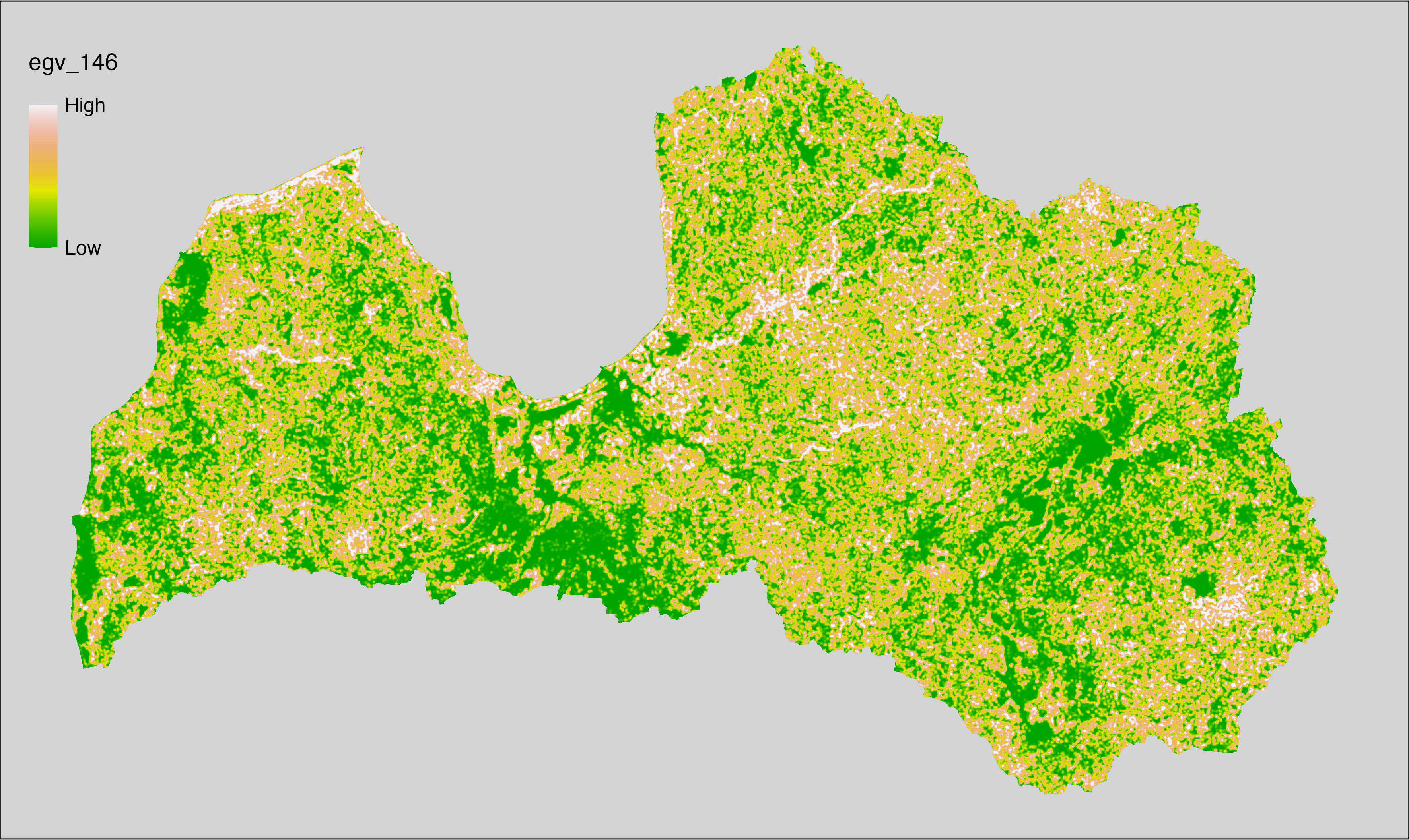
6.147 Edges_OldForests_r1250
filename: Edges_OldForests_r1250.tif
layername: egv_147
English name: Edge pixels of Forests Over Rotation Age within the 1.25 km landscape
Latvian name: Pieaugušo un pāraugušo mežaudžu malu pikseļu skaits 1,25 km ainavā
Procedure: The total edge within a 1250 m radius around the analysis grid cell is
calculated as the area-weighted sum of the analysis cells inside the
buffer, using the workflow egvtools::radius_function(). During the calculation of the landscape metric,
inverse distance weighted (power = 2) gap filling on the output is applied
to ensure no missing values at the edges. Then the layer is rewritten to set
its name. Finally, the layer is standardised by subtracting the arithmetic
mean and dividing by the root mean squared error.
Code
# libs ----
if(!require(terra)) {install.packages("terra"); require(terra)}
if(!require(egvtools)) {remotes::install_github("aavotins/egvtools"); require(egvtools)}
# Templates -----
template100=rast("./Templates/TemplateRasters/LV100m_10km.tif")
# radii ----
radius_function(
kvadrati_path = "./Templates/TemplateGrids/tiles/",
radii_path = "./Templates/TemplateGridPoints/tiles/",
tikls100_path = "./Templates/TemplateGrids/tikls100_sauzeme.parquet",
template_path = "./Templates/TemplateRasters/LV100m_10km.tif",
input_layers = c("./RasterGrids_100m/2024/RAW/Edges_OldForests_cell.tif"),
layer_prefixes = c("Edges_OldForests"),
output_dir = "./RasterGrids_100m/2024/RAW/",
n_workers = 12,
radii = c("r1250"),
radius_mode = "sparse",
extract_fun = "sum",
fill_missing = TRUE,
IDW_weight = 2,
future_max_size = 20 * 1024^3)
# Edges_OldForests_r1250.tif egv_147 ----
slanis=rast("./RasterGrids_100m/2024/RAW/Edges_OldForests_r1250.tif")
names(slanis)="egv_147"
slanis2=project(slanis,template100)
writeRaster(slanis2,
"./RasterGrids_100m/2024/RAW/Edges_OldForests_r1250.tif",
overwrite=TRUE)
# standardisation ----
if(!require(terra)) {install.packages("terra"); require(terra)}
if(!require(tidyverse)) {install.packages("tidyverse"); require(tidyverse)}
nosaukums="Edges_OldForests_r1250.tif"
ielasisanas_cels=paste0("./RasterGrids_100m/2024/RAW/",nosaukums)
saglabasanas_cels=paste0("./RasterGrids_100m/2024/Scaled/",nosaukums)
slanis=rast(ielasisanas_cels)
videjais=global(slanis,fun="mean",na.rm=TRUE)
centrets=slanis-videjais[,1]
standartnovirze=terra::global(centrets,fun="rms",na.rm=TRUE)
merogots=centrets/standartnovirze[,1]
writeRaster(merogots,
filename=saglabasanas_cels,
overwrite=TRUE)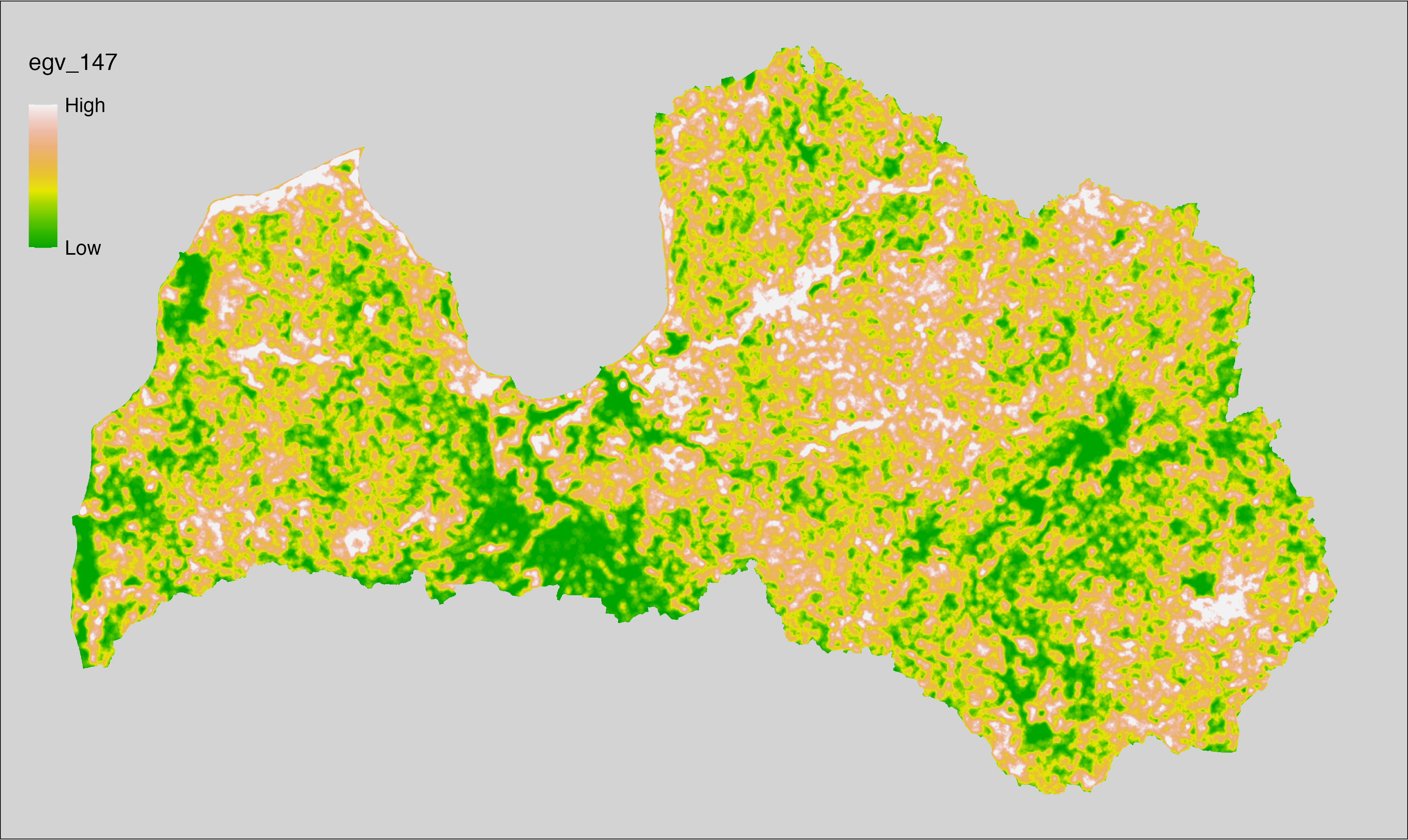
6.148 Edges_OldForests_r3000
filename: Edges_OldForests_r3000.tif
layername: egv_148
English name: Edge pixels of Forests Over Rotation Age within the 3 km landscape
Latvian name: Pieaugušo un pāraugušo mežaudžu malu pikseļu skaits 3 km ainavā
Procedure: The total edge within a 3000 m radius around the analysis grid cell is
calculated as the area-weighted sum of the analysis cells inside the
buffer, using the workflow egvtools::radius_function(). During the calculation of the landscape metric,
inverse distance weighted (power = 2) gap filling on the output is applied
to ensure no missing values at the edges. Then the layer is rewritten to set
its name. Finally, the layer is standardised by subtracting the arithmetic
mean and dividing by the root mean squared error.
Code
# libs ----
if(!require(terra)) {install.packages("terra"); require(terra)}
if(!require(egvtools)) {remotes::install_github("aavotins/egvtools"); require(egvtools)}
# Templates -----
template100=rast("./Templates/TemplateRasters/LV100m_10km.tif")
# radii ----
radius_function(
kvadrati_path = "./Templates/TemplateGrids/tiles/",
radii_path = "./Templates/TemplateGridPoints/tiles/",
tikls100_path = "./Templates/TemplateGrids/tikls100_sauzeme.parquet",
template_path = "./Templates/TemplateRasters/LV100m_10km.tif",
input_layers = c("./RasterGrids_100m/2024/RAW/Edges_OldForests_cell.tif"),
layer_prefixes = c("Edges_OldForests"),
output_dir = "./RasterGrids_100m/2024/RAW/",
n_workers = 12,
radii = c("r3000"),
radius_mode = "sparse",
extract_fun = "sum",
fill_missing = TRUE,
IDW_weight = 2,
future_max_size = 20 * 1024^3)
# Edges_OldForests_r3000.tif egv_148 ----
slanis=rast("./RasterGrids_100m/2024/RAW/Edges_OldForests_r3000.tif")
names(slanis)="egv_148"
slanis2=project(slanis,template100)
writeRaster(slanis2,
"./RasterGrids_100m/2024/RAW/Edges_OldForests_r3000.tif",
overwrite=TRUE)
# standardisation ----
if(!require(terra)) {install.packages("terra"); require(terra)}
if(!require(tidyverse)) {install.packages("tidyverse"); require(tidyverse)}
nosaukums="Edges_OldForests_r3000.tif"
ielasisanas_cels=paste0("./RasterGrids_100m/2024/RAW/",nosaukums)
saglabasanas_cels=paste0("./RasterGrids_100m/2024/Scaled/",nosaukums)
slanis=rast(ielasisanas_cels)
videjais=global(slanis,fun="mean",na.rm=TRUE)
centrets=slanis-videjais[,1]
standartnovirze=terra::global(centrets,fun="rms",na.rm=TRUE)
merogots=centrets/standartnovirze[,1]
writeRaster(merogots,
filename=saglabasanas_cels,
overwrite=TRUE)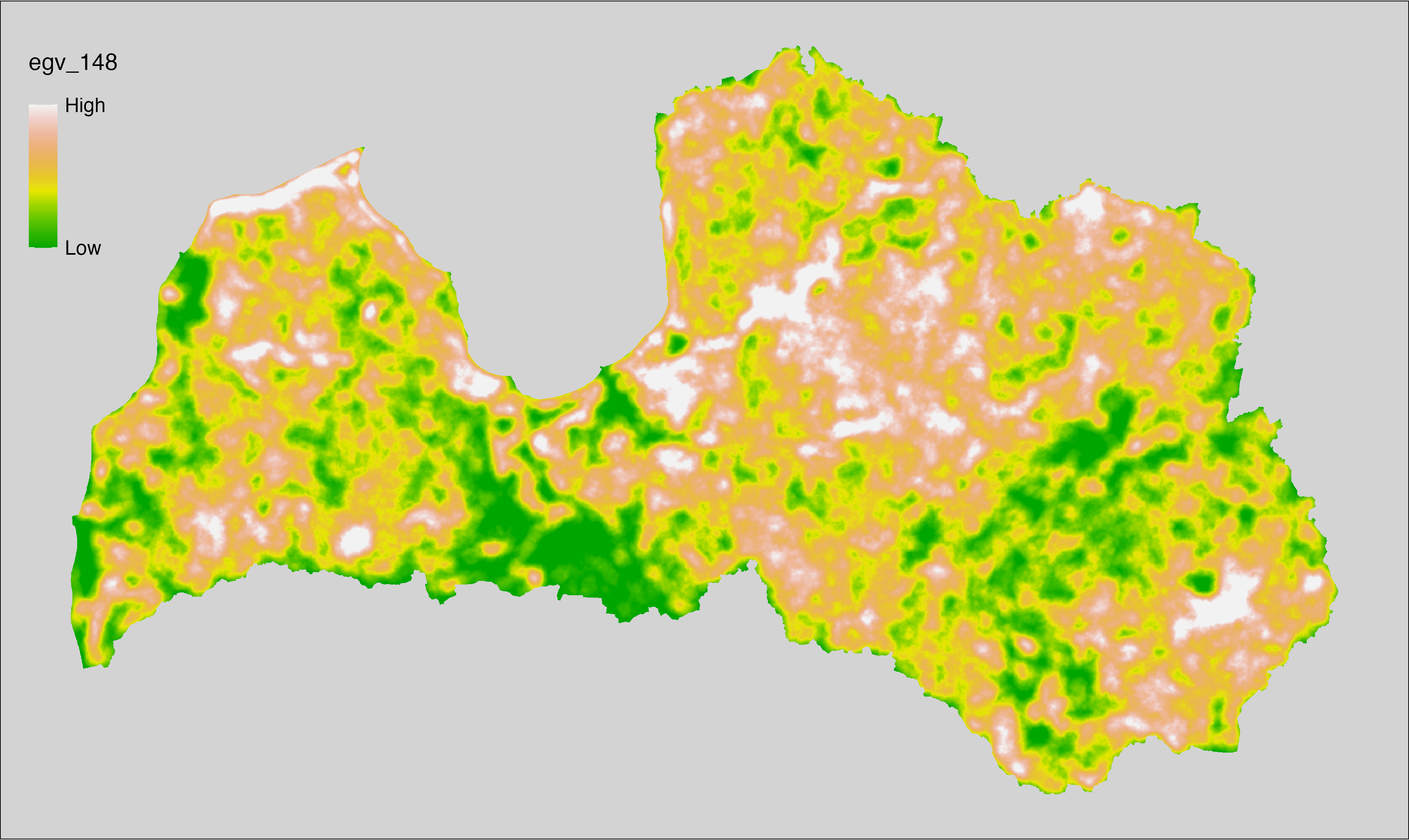
6.149 Edges_OldForests_r10000
filename: Edges_OldForests_r10000.tif
layername: egv_149
English name: Edge pixels of Forests Over Rotation Age within the 10 km landscape
Latvian name: Pieaugušo un pāraugušo mežaudžu malu pikseļu skaits 10 km ainavā
Procedure: The total edge within a 10000 m radius around the analysis grid cell is
calculated as the area-weighted sum of the analysis cells inside the
buffer, using the workflow egvtools::radius_function(). During the calculation of the landscape metric,
inverse distance weighted (power = 2) gap filling on the output is applied
to ensure no missing values at the edges. Then the layer is rewritten to set
its name. Finally, the layer is standardised by subtracting the arithmetic
mean and dividing by the root mean squared error.
Code
# libs ----
if(!require(terra)) {install.packages("terra"); require(terra)}
if(!require(egvtools)) {remotes::install_github("aavotins/egvtools"); require(egvtools)}
# Templates -----
template100=rast("./Templates/TemplateRasters/LV100m_10km.tif")
# radii ----
radius_function(
kvadrati_path = "./Templates/TemplateGrids/tiles/",
radii_path = "./Templates/TemplateGridPoints/tiles/",
tikls100_path = "./Templates/TemplateGrids/tikls100_sauzeme.parquet",
template_path = "./Templates/TemplateRasters/LV100m_10km.tif",
input_layers = c("./RasterGrids_100m/2024/RAW/Edges_OldForests_cell.tif"),
layer_prefixes = c("Edges_OldForests"),
output_dir = "./RasterGrids_100m/2024/RAW/",
n_workers = 12,
radii = c("r10000"),
radius_mode = "sparse",
extract_fun = "sum",
fill_missing = TRUE,
IDW_weight = 2,
future_max_size = 20 * 1024^3)
# Edges_OldForests_r10000.tif egv_149 ----
slanis=rast("./RasterGrids_100m/2024/RAW/Edges_OldForests_r10000.tif")
names(slanis)="egv_149"
slanis2=project(slanis,template100)
writeRaster(slanis2,
"./RasterGrids_100m/2024/RAW/Edges_OldForests_r10000.tif",
overwrite=TRUE)
# standardisation ----
if(!require(terra)) {install.packages("terra"); require(terra)}
if(!require(tidyverse)) {install.packages("tidyverse"); require(tidyverse)}
nosaukums="Edges_OldForests_r10000.tif"
ielasisanas_cels=paste0("./RasterGrids_100m/2024/RAW/",nosaukums)
saglabasanas_cels=paste0("./RasterGrids_100m/2024/Scaled/",nosaukums)
slanis=rast(ielasisanas_cels)
videjais=global(slanis,fun="mean",na.rm=TRUE)
centrets=slanis-videjais[,1]
standartnovirze=terra::global(centrets,fun="rms",na.rm=TRUE)
merogots=centrets/standartnovirze[,1]
writeRaster(merogots,
filename=saglabasanas_cels,
overwrite=TRUE)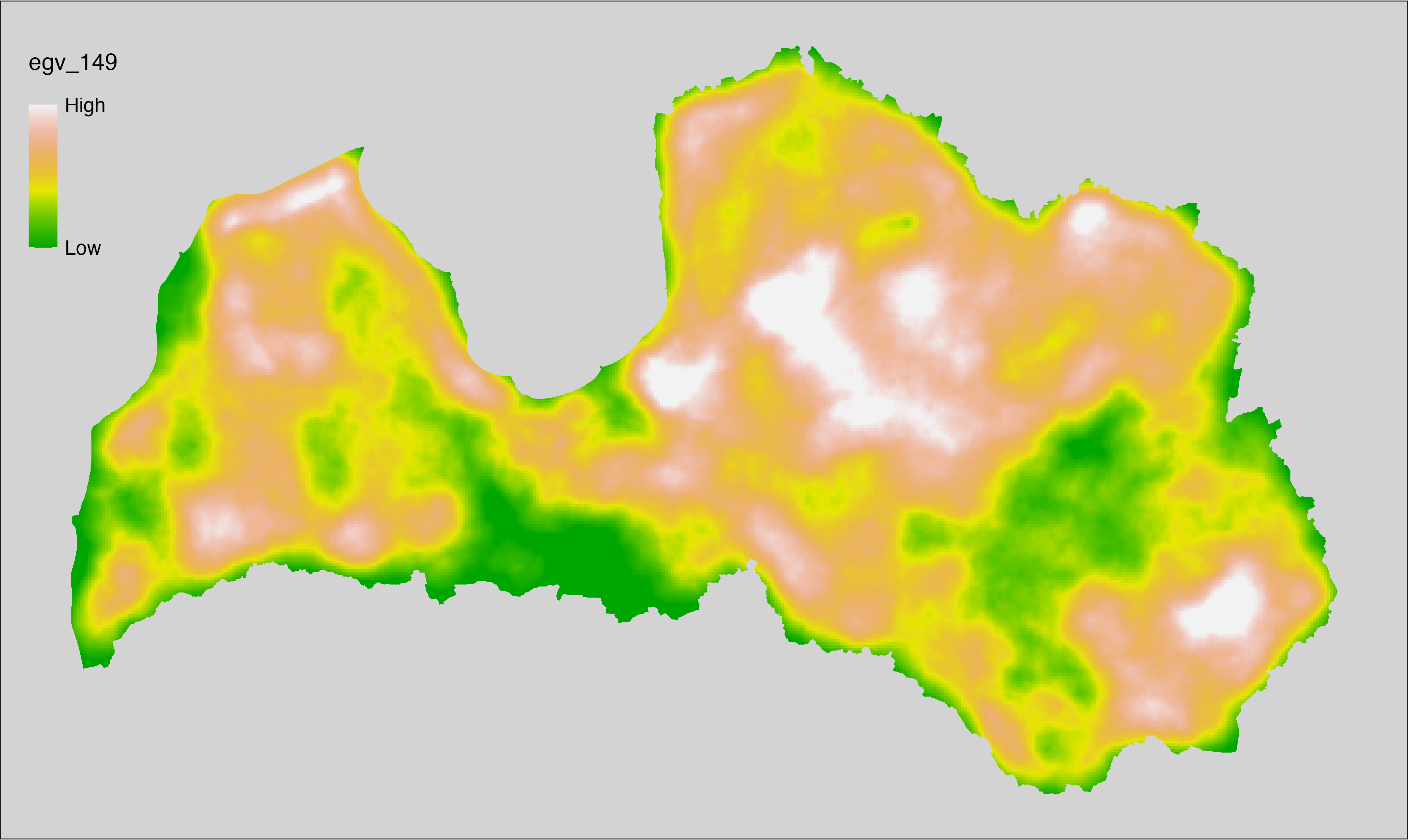
6.150 Edges_Roads_cell
filename: Edges_Roads_cell.tif
layername: egv_150
English name: Edge pixels of Roads within the analysis cell (1 ha)
Latvian name: Ceļu malu pikseļu skaits analīzes šūnā (1 ha)
Procedure: First, values equal to 100 from the Landscape
classification are coded as 1, and other values as NA. Then, the
layer (1 = presence) is covered over the nulls layer (presence = 0) and written to
file (matching the input). Next, with the workflow
egvtools::landscape_function() total edge between the two classes is
calculated. During the calculation of the landscape metric, inverse distance weighted
(power = 2) gap filling on the output is applied to ensure no missing values
at the edges. Finally, the layer is standardised by subtracting the arithmetic
mean and dividing by the root mean squared error.
Code
# libs ----
if(!require(terra)) {install.packages("terra"); require(terra)}
if(!require(egvtools)) {remotes::install_github("aavotins/egvtools"); require(egvtools)}
if(!require(sf)) {install.packages("sf"); require(sf)}
if(!require(sfarrow)) {install.packages("sfarrow"); require(sfarrow)}
if(!require(raster)) {install.packages("raster"); require(raster)}
if(!require(fasterize)) {install.packages("fasterize"); require(fasterize)}
if(!require(tidyverse)) {install.packages("tidyverse"); require(tidyverse)}
# Templates -----
template10=rast("./Templates/TemplateRasters/LV10m_10km.tif")
nulls10=rast("./Templates/TemplateRasters/nulls_LV10m_10km.tif")
# simple landscape ----
simple_landscape=rast("./RasterGrids_10m/2024/Ainava_vienk_mask.tif")
# Edges_Roads_input.tif ----
roads=ifel(simple_landscape==100,1,NA)
plot(roads)
roads=cover(roads,nulls10)
plot(roads)
edge_roads=project(roads,template10,
filename="./RasterGrids_10m/2024/Edges_Roads_input.tif",
overwrite=TRUE)
rm(edge_roads)
# Edges_Roads_cell.tif egv_150 ----
landscape_function(
landscape = "./RasterGrids_10m/2024/Edges_Roads_input.tif",
zones = "./Templates/TemplateGrids/tikls100_sauzeme.parquet",
id_field = "id",
tile_field = "tks50km",
template = "./Templates/TemplateRasters/LV100m_10km.tif",
out_dir = "./RasterGrids_100m/2024/RAW",
out_filename = "Edges_Roads_cell.tif",
out_layername = "egv_150",
what = "lsm_l_te",
lm_args = list(count_boundary = FALSE),
rasterize_engine = "fasterize",
n_workers = 12,
future_max_size = 20 * 1024^3,
fill_gaps = TRUE,
plot_gaps = FALSE,
plot_result = FALSE
)
# standardisation ----
if(!require(terra)) {install.packages("terra"); require(terra)}
if(!require(tidyverse)) {install.packages("tidyverse"); require(tidyverse)}
nosaukums="Edges_Roads_cell.tif"
ielasisanas_cels=paste0("./RasterGrids_100m/2024/RAW/",nosaukums)
saglabasanas_cels=paste0("./RasterGrids_100m/2024/Scaled/",nosaukums)
slanis=rast(ielasisanas_cels)
videjais=global(slanis,fun="mean",na.rm=TRUE)
centrets=slanis-videjais[,1]
standartnovirze=terra::global(centrets,fun="rms",na.rm=TRUE)
merogots=centrets/standartnovirze[,1]
writeRaster(merogots,
filename=saglabasanas_cels,
overwrite=TRUE)
6.151 Edges_Roads_r500
filename: Edges_Roads_r500.tif
layername: egv_151
English name: Edge pixels of Roads within the 0.5 km landscape
Latvian name: Ceļu malu pikseļu skaits 0,5 km ainavā
Procedure: The total edge within a 500 m radius around the analysis grid cell is
calculated as the area-weighted sum of the analysis cells inside the
buffer, using the workflow egvtools::radius_function(). During the calculation of the landscape metric,
inverse distance weighted (power = 2) gap filling on the output is applied
to ensure no missing values at the edges. Then the layer is rewritten to set
its name. Finally, the layer is standardised by subtracting the arithmetic
mean and dividing by the root mean squared error.
Code
# libs ----
if(!require(terra)) {install.packages("terra"); require(terra)}
if(!require(egvtools)) {remotes::install_github("aavotins/egvtools"); require(egvtools)}
# Templates -----
template100=rast("./Templates/TemplateRasters/LV100m_10km.tif")
# radii ----
radius_function(
kvadrati_path = "./Templates/TemplateGrids/tiles/",
radii_path = "./Templates/TemplateGridPoints/tiles/",
tikls100_path = "./Templates/TemplateGrids/tikls100_sauzeme.parquet",
template_path = "./Templates/TemplateRasters/LV100m_10km.tif",
input_layers = c("./RasterGrids_100m/2024/RAW/Edges_Roads_cell.tif"),
layer_prefixes = c("Edges_Roads"),
output_dir = "./RasterGrids_100m/2024/RAW/",
n_workers = 12,
radii = c("r500"),
radius_mode = "sparse",
extract_fun = "sum",
fill_missing = TRUE,
IDW_weight = 2,
future_max_size = 20 * 1024^3)
# Edges_Roads_r500.tif egv_151 ----
slanis=rast("./RasterGrids_100m/2024/RAW/Edges_Roads_r500.tif")
names(slanis)="egv_151"
slanis2=project(slanis,template100)
writeRaster(slanis2,
"./RasterGrids_100m/2024/RAW/Edges_Roads_r500.tif",
overwrite=TRUE)
# standardisation ----
if(!require(terra)) {install.packages("terra"); require(terra)}
if(!require(tidyverse)) {install.packages("tidyverse"); require(tidyverse)}
nosaukums="Edges_Roads_r500.tif"
ielasisanas_cels=paste0("./RasterGrids_100m/2024/RAW/",nosaukums)
saglabasanas_cels=paste0("./RasterGrids_100m/2024/Scaled/",nosaukums)
slanis=rast(ielasisanas_cels)
videjais=global(slanis,fun="mean",na.rm=TRUE)
centrets=slanis-videjais[,1]
standartnovirze=terra::global(centrets,fun="rms",na.rm=TRUE)
merogots=centrets/standartnovirze[,1]
writeRaster(merogots,
filename=saglabasanas_cels,
overwrite=TRUE)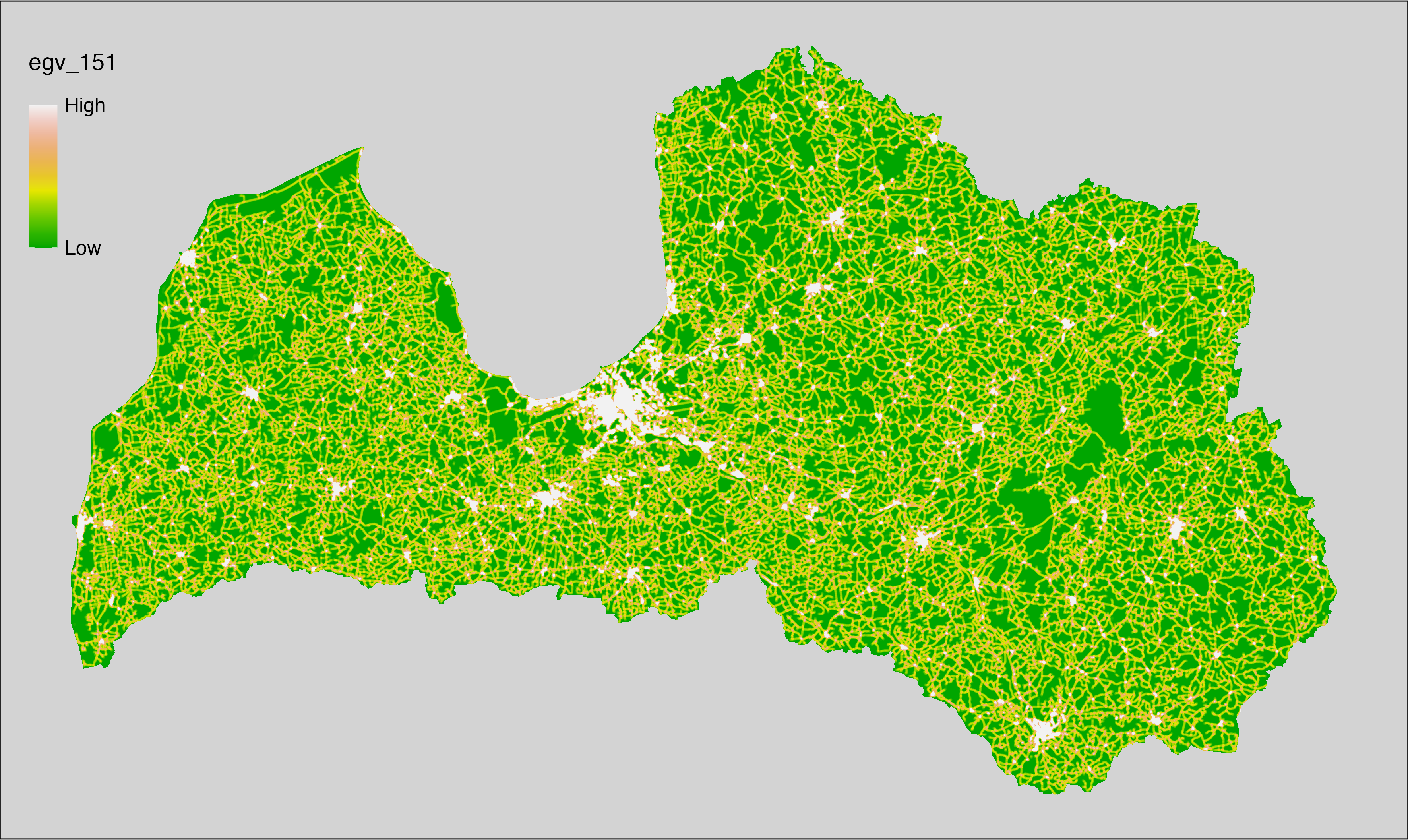
6.152 Edges_Roads_r1250
filename: Edges_Roads_r1250.tif
layername: egv_152
English name: Edge pixels of Roads within the 1.25 km landscape
Latvian name: Ceļu malu pikseļu skaits 1,25 km ainavā
Procedure: The total edge within a 1250 m radius around the analysis grid cell is
calculated as the area-weighted sum of the analysis cells inside the
buffer, using the workflow egvtools::radius_function(). During the calculation of the landscape metric,
inverse distance weighted (power = 2) gap filling on the output is applied
to ensure no missing values at the edges. Then the layer is rewritten to set
its name. Finally, the layer is standardised by subtracting the arithmetic
mean and dividing by the root mean squared error.
Code
# libs ----
if(!require(terra)) {install.packages("terra"); require(terra)}
if(!require(egvtools)) {remotes::install_github("aavotins/egvtools"); require(egvtools)}
# Templates -----
template100=rast("./Templates/TemplateRasters/LV100m_10km.tif")
# radii ----
radius_function(
kvadrati_path = "./Templates/TemplateGrids/tiles/",
radii_path = "./Templates/TemplateGridPoints/tiles/",
tikls100_path = "./Templates/TemplateGrids/tikls100_sauzeme.parquet",
template_path = "./Templates/TemplateRasters/LV100m_10km.tif",
input_layers = c("./RasterGrids_100m/2024/RAW/Edges_Roads_cell.tif"),
layer_prefixes = c("Edges_Roads"),
output_dir = "./RasterGrids_100m/2024/RAW/",
n_workers = 12,
radii = c("r1250"),
radius_mode = "sparse",
extract_fun = "sum",
fill_missing = TRUE,
IDW_weight = 2,
future_max_size = 20 * 1024^3)
# Edges_Roads_r1250.tif egv_152 ----
slanis=rast("./RasterGrids_100m/2024/RAW/Edges_Roads_r1250.tif")
names(slanis)="egv_152"
slanis2=project(slanis,template100)
writeRaster(slanis2,
"./RasterGrids_100m/2024/RAW/Edges_Roads_r1250.tif",
overwrite=TRUE)
# standardisation ----
if(!require(terra)) {install.packages("terra"); require(terra)}
if(!require(tidyverse)) {install.packages("tidyverse"); require(tidyverse)}
nosaukums="Edges_Roads_r1250.tif"
ielasisanas_cels=paste0("./RasterGrids_100m/2024/RAW/",nosaukums)
saglabasanas_cels=paste0("./RasterGrids_100m/2024/Scaled/",nosaukums)
slanis=rast(ielasisanas_cels)
videjais=global(slanis,fun="mean",na.rm=TRUE)
centrets=slanis-videjais[,1]
standartnovirze=terra::global(centrets,fun="rms",na.rm=TRUE)
merogots=centrets/standartnovirze[,1]
writeRaster(merogots,
filename=saglabasanas_cels,
overwrite=TRUE)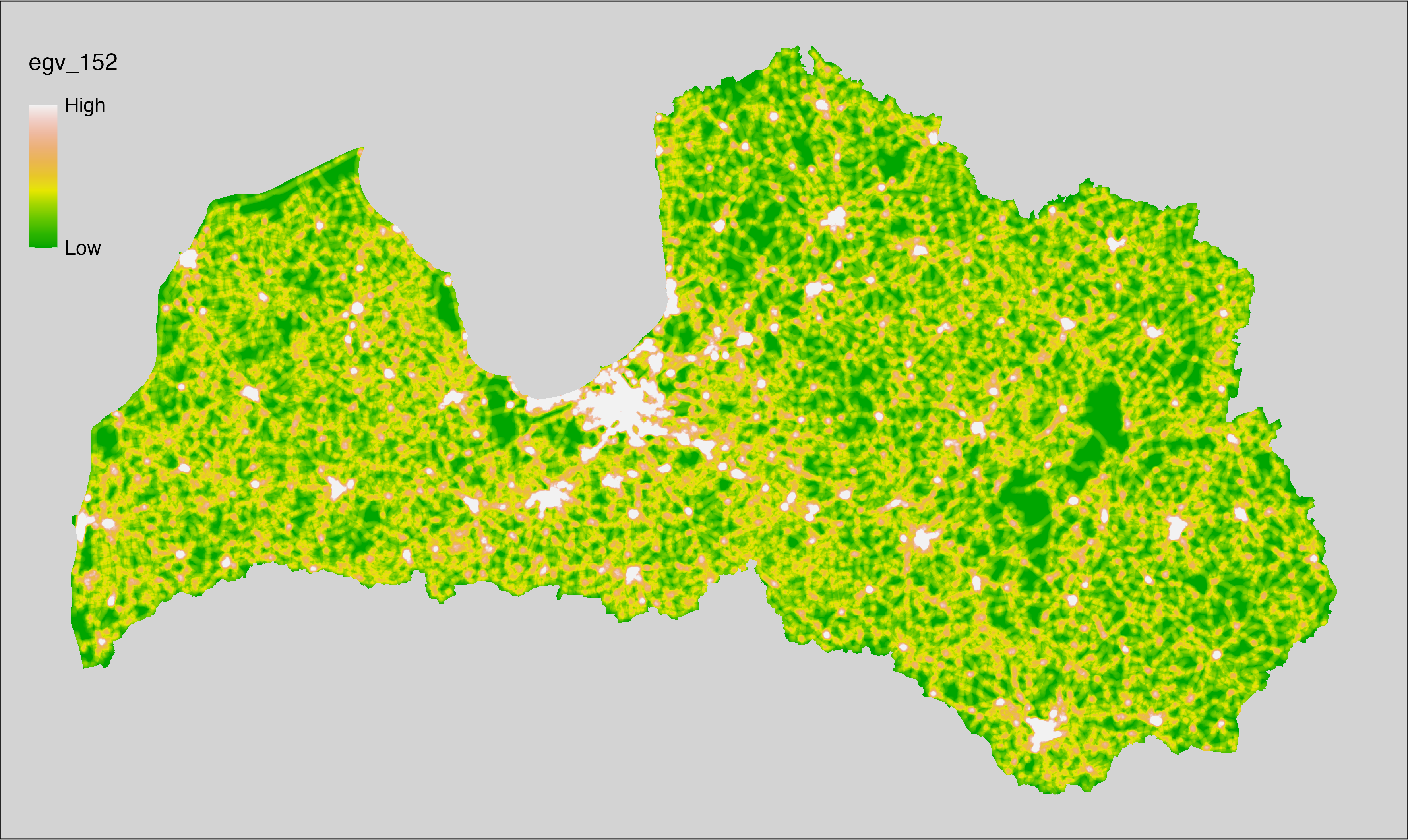
6.153 Edges_Roads_r3000
filename: Edges_Roads_r3000.tif
layername: egv_153
English name: Edge pixels of Roads within the 3 km landscape
Latvian name: Ceļu malu pikseļu skaits 3 km ainavā
Procedure: The total edge within a 3000 m radius around the analysis grid cell is
calculated as the area-weighted sum of the analysis cells inside the
buffer, using the workflow egvtools::radius_function(). During the calculation of the landscape metric,
inverse distance weighted (power = 2) gap filling on the output is applied
to ensure no missing values at the edges. Then the layer is rewritten to set
its name. Finally, the layer is standardised by subtracting the arithmetic
mean and dividing by the root mean squared error.
Code
# libs ----
if(!require(terra)) {install.packages("terra"); require(terra)}
if(!require(egvtools)) {remotes::install_github("aavotins/egvtools"); require(egvtools)}
# Templates -----
template100=rast("./Templates/TemplateRasters/LV100m_10km.tif")
# radii ----
radius_function(
kvadrati_path = "./Templates/TemplateGrids/tiles/",
radii_path = "./Templates/TemplateGridPoints/tiles/",
tikls100_path = "./Templates/TemplateGrids/tikls100_sauzeme.parquet",
template_path = "./Templates/TemplateRasters/LV100m_10km.tif",
input_layers = c("./RasterGrids_100m/2024/RAW/Edges_Roads_cell.tif"),
layer_prefixes = c("Edges_Roads"),
output_dir = "./RasterGrids_100m/2024/RAW/",
n_workers = 12,
radii = c("r3000"),
radius_mode = "sparse",
extract_fun = "sum",
fill_missing = TRUE,
IDW_weight = 2,
future_max_size = 20 * 1024^3)
# Edges_Roads_r3000.tif egv_153 ----
slanis=rast("./RasterGrids_100m/2024/RAW/Edges_Roads_r3000.tif")
names(slanis)="egv_153"
slanis2=project(slanis,template100)
writeRaster(slanis2,
"./RasterGrids_100m/2024/RAW/Edges_Roads_r3000.tif",
overwrite=TRUE)
# standardisation ----
if(!require(terra)) {install.packages("terra"); require(terra)}
if(!require(tidyverse)) {install.packages("tidyverse"); require(tidyverse)}
nosaukums="Edges_Roads_r3000.tif"
ielasisanas_cels=paste0("./RasterGrids_100m/2024/RAW/",nosaukums)
saglabasanas_cels=paste0("./RasterGrids_100m/2024/Scaled/",nosaukums)
slanis=rast(ielasisanas_cels)
videjais=global(slanis,fun="mean",na.rm=TRUE)
centrets=slanis-videjais[,1]
standartnovirze=terra::global(centrets,fun="rms",na.rm=TRUE)
merogots=centrets/standartnovirze[,1]
writeRaster(merogots,
filename=saglabasanas_cels,
overwrite=TRUE)
6.154 Edges_Roads_r10000
filename: Edges_Roads_r10000.tif
layername: egv_154
English name: Edge pixels of Roads within the 10 km landscape
Latvian name: Ceļu malu pikseļu skaits 10 km ainavā
Procedure: The total edge within a 10000 m radius around the analysis grid cell is
calculated as the area-weighted sum of the analysis cells inside the
buffer, using the workflow egvtools::radius_function(). During the calculation of the landscape metric,
inverse distance weighted (power = 2) gap filling on the output is applied
to ensure no missing values at the edges. Then the layer is rewritten to set
its name. Finally, the layer is standardised by subtracting the arithmetic
mean and dividing by the root mean squared error.
Code
# libs ----
if(!require(terra)) {install.packages("terra"); require(terra)}
if(!require(egvtools)) {remotes::install_github("aavotins/egvtools"); require(egvtools)}
# Templates -----
template100=rast("./Templates/TemplateRasters/LV100m_10km.tif")
# radii ----
radius_function(
kvadrati_path = "./Templates/TemplateGrids/tiles/",
radii_path = "./Templates/TemplateGridPoints/tiles/",
tikls100_path = "./Templates/TemplateGrids/tikls100_sauzeme.parquet",
template_path = "./Templates/TemplateRasters/LV100m_10km.tif",
input_layers = c("./RasterGrids_100m/2024/RAW/Edges_Roads_cell.tif"),
layer_prefixes = c("Edges_Roads"),
output_dir = "./RasterGrids_100m/2024/RAW/",
n_workers = 12,
radii = c("r10000"),
radius_mode = "sparse",
extract_fun = "sum",
fill_missing = TRUE,
IDW_weight = 2,
future_max_size = 20 * 1024^3)
# Edges_Roads_r10000.tif egv_154 ----
slanis=rast("./RasterGrids_100m/2024/RAW/Edges_Roads_r10000.tif")
names(slanis)="egv_154"
slanis2=project(slanis,template100)
writeRaster(slanis2,
"./RasterGrids_100m/2024/RAW/Edges_Roads_r10000.tif",
overwrite=TRUE)
# standardisation ----
if(!require(terra)) {install.packages("terra"); require(terra)}
if(!require(tidyverse)) {install.packages("tidyverse"); require(tidyverse)}
nosaukums="Edges_Roads_r10000.tif"
ielasisanas_cels=paste0("./RasterGrids_100m/2024/RAW/",nosaukums)
saglabasanas_cels=paste0("./RasterGrids_100m/2024/Scaled/",nosaukums)
slanis=rast(ielasisanas_cels)
videjais=global(slanis,fun="mean",na.rm=TRUE)
centrets=slanis-videjais[,1]
standartnovirze=terra::global(centrets,fun="rms",na.rm=TRUE)
merogots=centrets/standartnovirze[,1]
writeRaster(merogots,
filename=saglabasanas_cels,
overwrite=TRUE)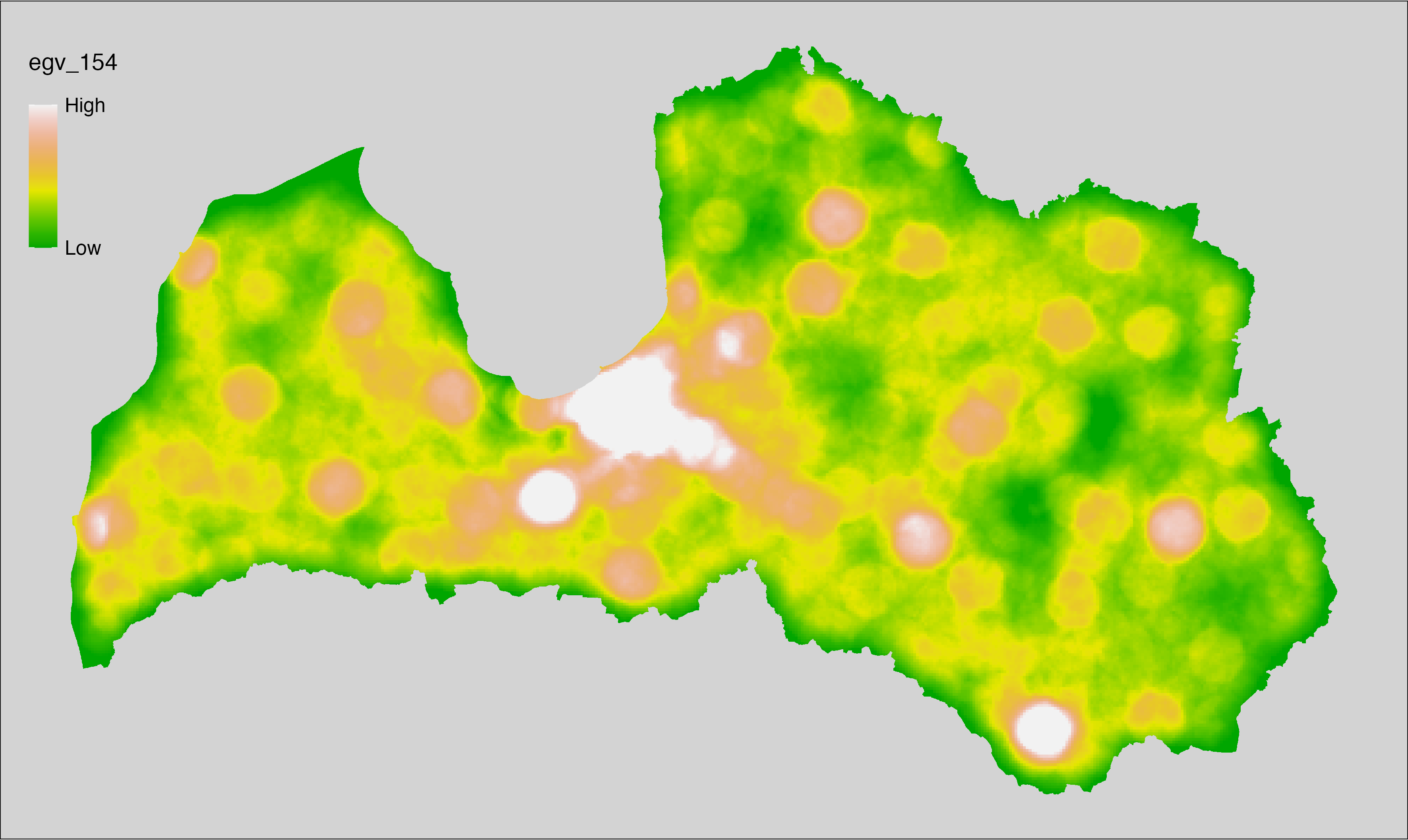
6.155 Edges_Trees_cell
filename: Edges_Trees_cell.tif
layername: egv_155
English name: Edge pixels of Trees within the analysis cell (1 ha)
Latvian name: Koku malu pikseļu skaits analīzes šūnā (1 ha)
Procedure: First, values larger or equal to 630 and smaller than 700 from
Landscape classification are coded as 1, and all other values as NA.
Then, the layer (1 = presence) is covered over the nulls layer (presence = 0) and
written to file (matching the input). Next, with the workflow
egvtools::landscape_function() total edge between the two classes is
calculated. During the calculation of the landscape metric, inverse distance weighted
(power = 2) gap filling on the output is applied to ensure no missing values
at the edges. Finally, the layer is standardised by subtracting the arithmetic
mean and dividing by the root mean squared error.
Code
# libs ----
if(!require(terra)) {install.packages("terra"); require(terra)}
if(!require(egvtools)) {remotes::install_github("aavotins/egvtools"); require(egvtools)}
if(!require(sf)) {install.packages("sf"); require(sf)}
if(!require(sfarrow)) {install.packages("sfarrow"); require(sfarrow)}
if(!require(raster)) {install.packages("raster"); require(raster)}
if(!require(fasterize)) {install.packages("fasterize"); require(fasterize)}
if(!require(tidyverse)) {install.packages("tidyverse"); require(tidyverse)}
# Templates -----
template10=rast("./Templates/TemplateRasters/LV10m_10km.tif")
nulls10=rast("./Templates/TemplateRasters/nulls_LV10m_10km.tif")
# simple landscape ----
simple_landscape=rast("./RasterGrids_10m/2024/Ainava_vienk_mask.tif")
# Edges_Trees_input.tif ----
trees_from630=ifel(simple_landscape>=630 & simple_landscape<700,1,NA)
plot(trees_from630)
trees_from630=cover(trees_from630,nulls10)
plot(trees_from630)
edge_trees_from630=project(trees_from630,template10,
filename="./RasterGrids_10m/2024/Edges_Trees_input.tif",
overwrite=TRUE)
rm(edge_trees_from630)
# Edges_Trees_cell.tif egv_155
landscape_function(
landscape = "./RasterGrids_10m/2024/Edges_Trees_input.tif",
zones = "./Templates/TemplateGrids/tikls100_sauzeme.parquet",
id_field = "id",
tile_field = "tks50km",
template = "./Templates/TemplateRasters/LV100m_10km.tif",
out_dir = "./RasterGrids_100m/2024/RAW",
out_filename = "Edges_Trees_cell.tif",
out_layername = "egv_155",
what = "lsm_l_te",
lm_args = list(count_boundary = FALSE),
rasterize_engine = "fasterize",
n_workers = 12,
future_max_size = 20 * 1024^3,
fill_gaps = TRUE,
plot_gaps = FALSE,
plot_result = FALSE
)
# standardisation ----
if(!require(terra)) {install.packages("terra"); require(terra)}
if(!require(tidyverse)) {install.packages("tidyverse"); require(tidyverse)}
nosaukums="Edges_Trees_cell.tif"
ielasisanas_cels=paste0("./RasterGrids_100m/2024/RAW/",nosaukums)
saglabasanas_cels=paste0("./RasterGrids_100m/2024/Scaled/",nosaukums)
slanis=rast(ielasisanas_cels)
videjais=global(slanis,fun="mean",na.rm=TRUE)
centrets=slanis-videjais[,1]
standartnovirze=terra::global(centrets,fun="rms",na.rm=TRUE)
merogots=centrets/standartnovirze[,1]
writeRaster(merogots,
filename=saglabasanas_cels,
overwrite=TRUE)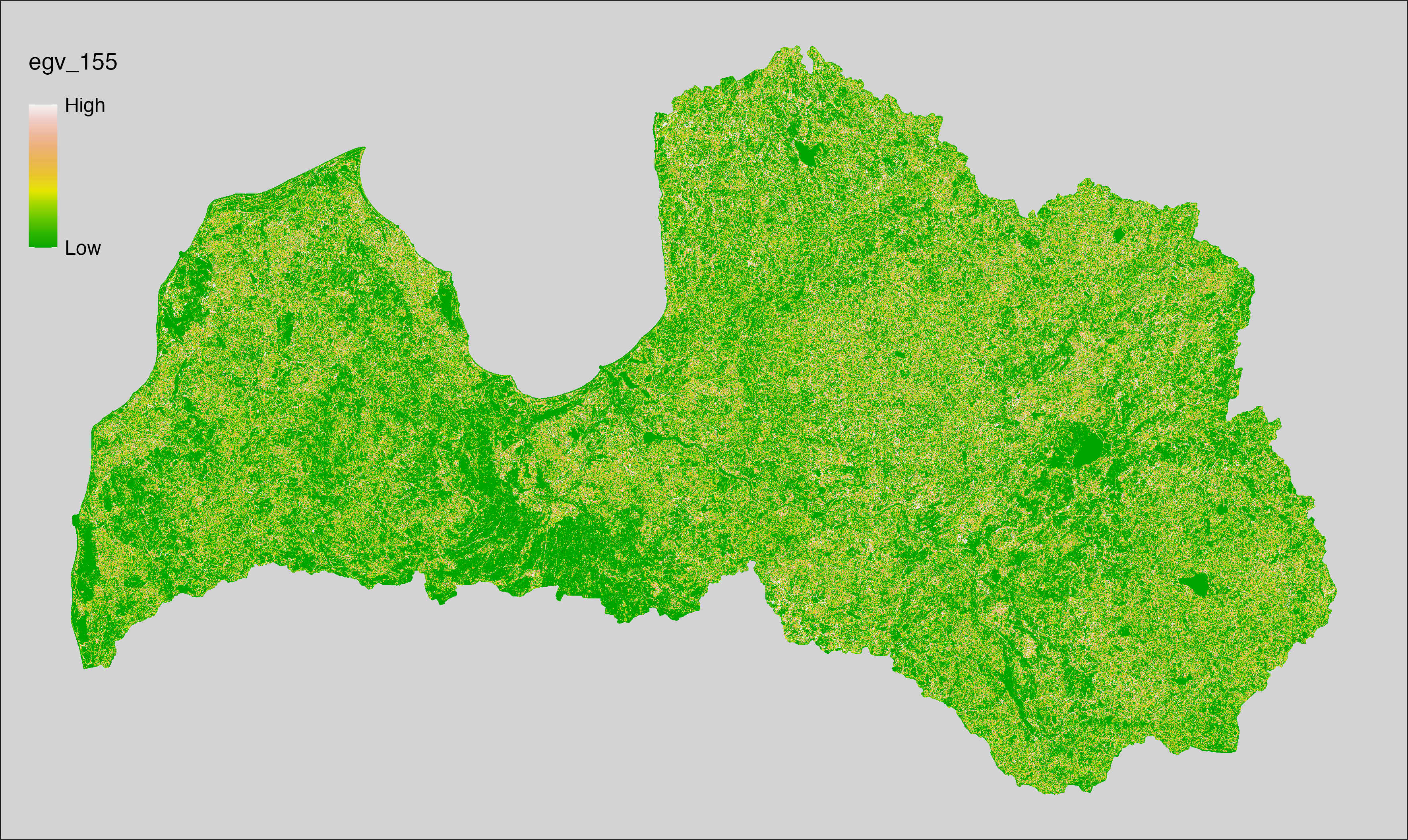
6.156 Edges_Trees_r500
filename: Edges_Trees_r500.tif
layername: egv_156
English name: Edge pixels of Trees within the 0.5 km landscape
Latvian name: Koku malu pikseļu skaits 0,5 km ainavā
Procedure: The total edge within a 500 m radius around the analysis grid cell is
calculated as the area-weighted sum of the analysis cells inside the
buffer, using the workflow egvtools::radius_function(). During the calculation of the landscape metric,
inverse distance weighted (power = 2) gap filling on the output is applied
to ensure no missing values at the edges. Then the layer is rewritten to set
its name. Finally, the layer is standardised by subtracting the arithmetic
mean and dividing by the root mean squared error.
Code
# libs ----
if(!require(terra)) {install.packages("terra"); require(terra)}
if(!require(egvtools)) {remotes::install_github("aavotins/egvtools"); require(egvtools)}
# Templates -----
template100=rast("./Templates/TemplateRasters/LV100m_10km.tif")
# radii ----
radius_function(
kvadrati_path = "./Templates/TemplateGrids/tiles/",
radii_path = "./Templates/TemplateGridPoints/tiles/",
tikls100_path = "./Templates/TemplateGrids/tikls100_sauzeme.parquet",
template_path = "./Templates/TemplateRasters/LV100m_10km.tif",
input_layers = c("./RasterGrids_100m/2024/RAW/Edges_Trees_cell.tif"),
layer_prefixes = c("Edges_Trees"),
output_dir = "./RasterGrids_100m/2024/RAW/",
n_workers = 12,
radii = c("r500"),
radius_mode = "sparse",
extract_fun = "sum",
fill_missing = TRUE,
IDW_weight = 2,
future_max_size = 20 * 1024^3)
# Edges_Trees_r500.tif egv_156 ----
slanis=rast("./RasterGrids_100m/2024/RAW/Edges_Trees_r500.tif")
names(slanis)="egv_156"
slanis2=project(slanis,template100)
writeRaster(slanis2,
"./RasterGrids_100m/2024/RAW/Edges_Trees_r500.tif",
overwrite=TRUE)
# standardisation ----
if(!require(terra)) {install.packages("terra"); require(terra)}
if(!require(tidyverse)) {install.packages("tidyverse"); require(tidyverse)}
nosaukums="Edges_Trees_r500.tif"
ielasisanas_cels=paste0("./RasterGrids_100m/2024/RAW/",nosaukums)
saglabasanas_cels=paste0("./RasterGrids_100m/2024/Scaled/",nosaukums)
slanis=rast(ielasisanas_cels)
videjais=global(slanis,fun="mean",na.rm=TRUE)
centrets=slanis-videjais[,1]
standartnovirze=terra::global(centrets,fun="rms",na.rm=TRUE)
merogots=centrets/standartnovirze[,1]
writeRaster(merogots,
filename=saglabasanas_cels,
overwrite=TRUE)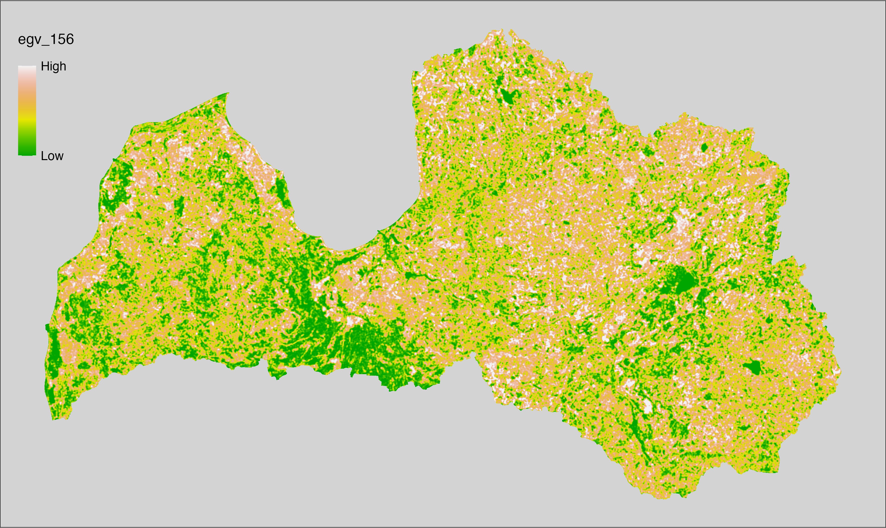
6.157 Edges_Trees_r1250
filename: Edges_Trees_r1250.tif
layername: egv_157
English name: Edge pixels of Trees within the 1.25 km landscape
Latvian name: Koku malu pikseļu skaits 1,25 km ainavā
Procedure: The total edge within a 1250 m radius around the analysis grid cell is
calculated as the area-weighted sum of the analysis cells inside the
buffer, using the workflow egvtools::radius_function(). During the calculation of the landscape metric,
inverse distance weighted (power = 2) gap filling on the output is applied
to ensure no missing values at the edges. Then the layer is rewritten to set
its name. Finally, the layer is standardised by subtracting the arithmetic
mean and dividing by the root mean squared error.
Code
# libs ----
if(!require(terra)) {install.packages("terra"); require(terra)}
if(!require(egvtools)) {remotes::install_github("aavotins/egvtools"); require(egvtools)}
# Templates -----
template100=rast("./Templates/TemplateRasters/LV100m_10km.tif")
# radii ----
radius_function(
kvadrati_path = "./Templates/TemplateGrids/tiles/",
radii_path = "./Templates/TemplateGridPoints/tiles/",
tikls100_path = "./Templates/TemplateGrids/tikls100_sauzeme.parquet",
template_path = "./Templates/TemplateRasters/LV100m_10km.tif",
input_layers = c("./RasterGrids_100m/2024/RAW/Edges_Trees_cell.tif"),
layer_prefixes = c("Edges_Trees"),
output_dir = "./RasterGrids_100m/2024/RAW/",
n_workers = 12,
radii = c("r1250"),
radius_mode = "sparse",
extract_fun = "sum",
fill_missing = TRUE,
IDW_weight = 2,
future_max_size = 20 * 1024^3)
# Edges_Trees_r1250.tif egv_157 ----
slanis=rast("./RasterGrids_100m/2024/RAW/Edges_Trees_r1250.tif")
names(slanis)="egv_157"
slanis2=project(slanis,template100)
writeRaster(slanis2,
"./RasterGrids_100m/2024/RAW/Edges_Trees_r1250.tif",
overwrite=TRUE)
# standardisation ----
if(!require(terra)) {install.packages("terra"); require(terra)}
if(!require(tidyverse)) {install.packages("tidyverse"); require(tidyverse)}
nosaukums="Edges_Trees_r1250.tif"
ielasisanas_cels=paste0("./RasterGrids_100m/2024/RAW/",nosaukums)
saglabasanas_cels=paste0("./RasterGrids_100m/2024/Scaled/",nosaukums)
slanis=rast(ielasisanas_cels)
videjais=global(slanis,fun="mean",na.rm=TRUE)
centrets=slanis-videjais[,1]
standartnovirze=terra::global(centrets,fun="rms",na.rm=TRUE)
merogots=centrets/standartnovirze[,1]
writeRaster(merogots,
filename=saglabasanas_cels,
overwrite=TRUE)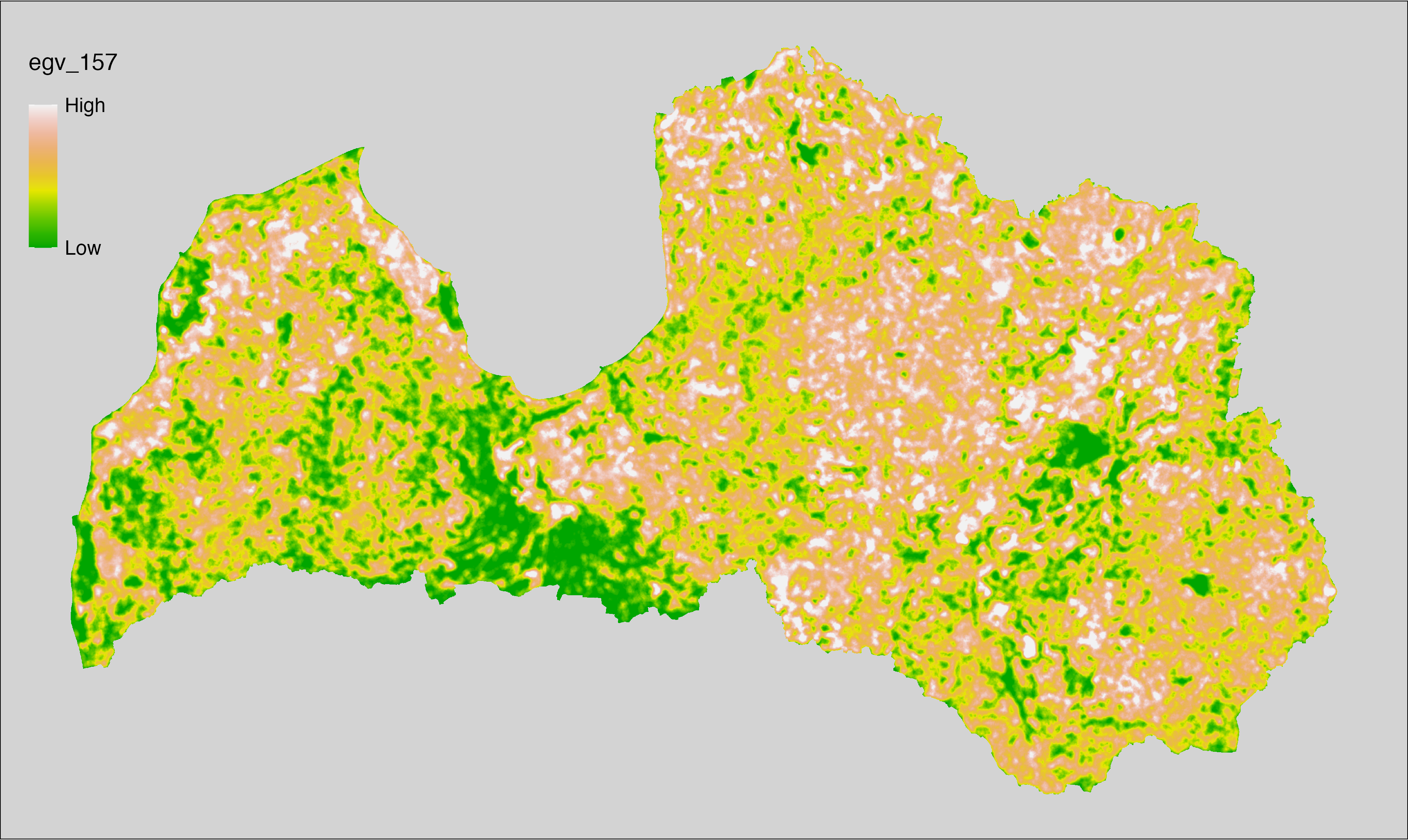
6.158 Edges_Trees_r3000
filename: Edges_Trees_r3000.tif
layername: egv_158
English name: Edge pixels of Trees within the 3 km landscape
Latvian name: Koku malu pikseļu skaits 3 km ainavā
Procedure: The total edge within a 3000 m radius around the analysis grid cell is
calculated as the area-weighted sum of the analysis cells inside the
buffer, using the workflow egvtools::radius_function(). During the calculation of the landscape metric,
inverse distance weighted (power = 2) gap filling on the output is applied
to ensure no missing values at the edges. Then the layer is rewritten to set
its name. Finally, the layer is standardised by subtracting the arithmetic
mean and dividing by the root mean squared error.
Code
# libs ----
if(!require(terra)) {install.packages("terra"); require(terra)}
if(!require(egvtools)) {remotes::install_github("aavotins/egvtools"); require(egvtools)}
# Templates -----
template100=rast("./Templates/TemplateRasters/LV100m_10km.tif")
# radii ----
radius_function(
kvadrati_path = "./Templates/TemplateGrids/tiles/",
radii_path = "./Templates/TemplateGridPoints/tiles/",
tikls100_path = "./Templates/TemplateGrids/tikls100_sauzeme.parquet",
template_path = "./Templates/TemplateRasters/LV100m_10km.tif",
input_layers = c("./RasterGrids_100m/2024/RAW/Edges_Trees_cell.tif"),
layer_prefixes = c("Edges_Trees"),
output_dir = "./RasterGrids_100m/2024/RAW/",
n_workers = 12,
radii = c("r3000"),
radius_mode = "sparse",
extract_fun = "sum",
fill_missing = TRUE,
IDW_weight = 2,
future_max_size = 20 * 1024^3)
# Edges_Trees_r3000.tif egv_158 ----
slanis=rast("./RasterGrids_100m/2024/RAW/Edges_Trees_r3000.tif")
names(slanis)="egv_158"
slanis2=project(slanis,template100)
writeRaster(slanis2,
"./RasterGrids_100m/2024/RAW/Edges_Trees_r3000.tif",
overwrite=TRUE)
# standardisation ----
if(!require(terra)) {install.packages("terra"); require(terra)}
if(!require(tidyverse)) {install.packages("tidyverse"); require(tidyverse)}
nosaukums="Edges_Trees_r3000.tif"
ielasisanas_cels=paste0("./RasterGrids_100m/2024/RAW/",nosaukums)
saglabasanas_cels=paste0("./RasterGrids_100m/2024/Scaled/",nosaukums)
slanis=rast(ielasisanas_cels)
videjais=global(slanis,fun="mean",na.rm=TRUE)
centrets=slanis-videjais[,1]
standartnovirze=terra::global(centrets,fun="rms",na.rm=TRUE)
merogots=centrets/standartnovirze[,1]
writeRaster(merogots,
filename=saglabasanas_cels,
overwrite=TRUE)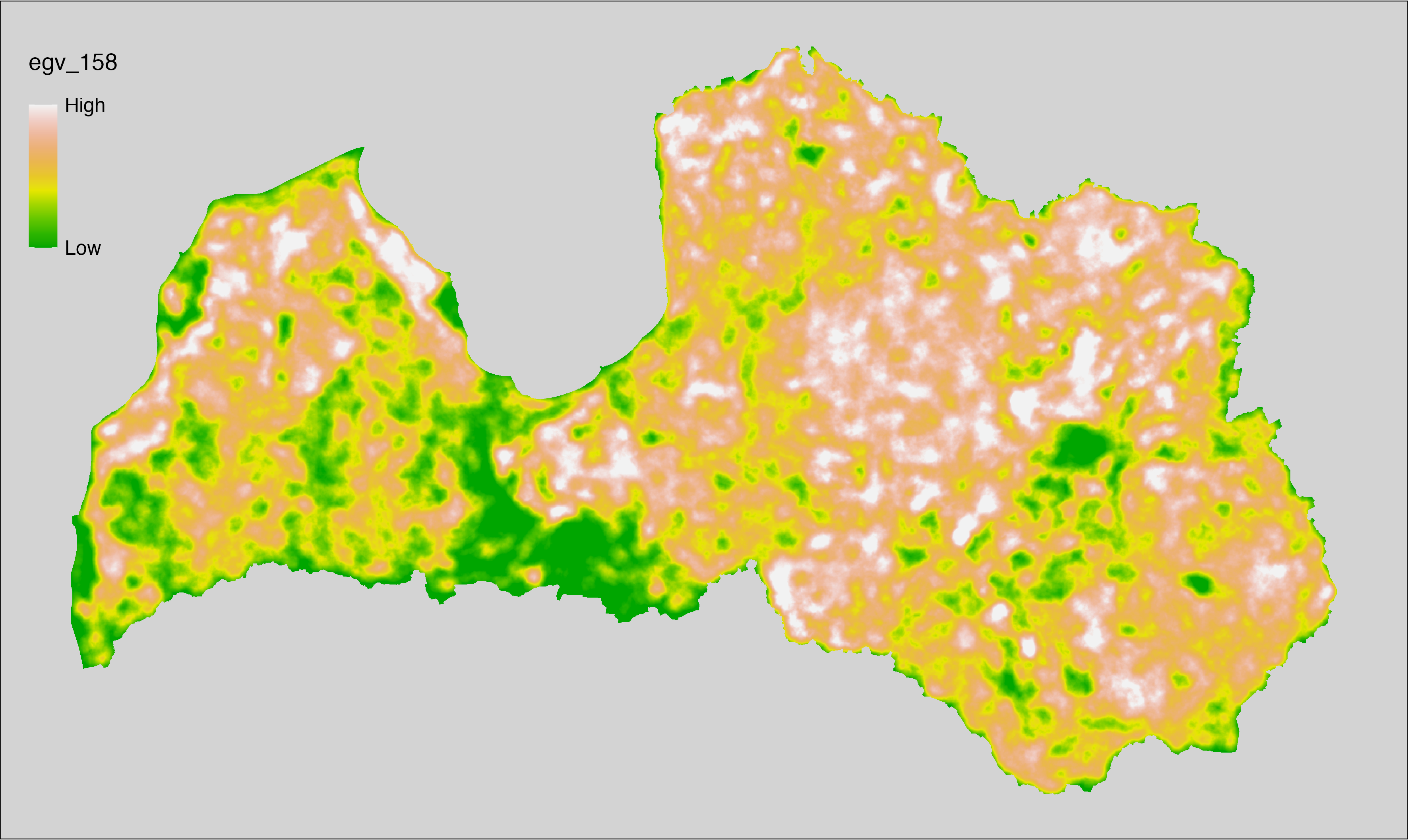
6.159 Edges_Trees_r10000
filename: Edges_Trees_r10000.tif
layername: egv_159
English name: Edge pixels of Trees within the 10 km landscape
Latvian name: Koku malu pikseļu skaits 10 km ainavā
Procedure: The total edge within a 10000 m radius around the analysis grid cell is
calculated as the area-weighted sum of the analysis cells inside the
buffer, using the workflow egvtools::radius_function(). During the calculation of the landscape metric,
inverse distance weighted (power = 2) gap filling on the output is applied
to ensure no missing values at the edges. Then the layer is rewritten to set
its name. Finally, the layer is standardised by subtracting the arithmetic
mean and dividing by the root mean squared error.
Code
# libs ----
if(!require(terra)) {install.packages("terra"); require(terra)}
if(!require(egvtools)) {remotes::install_github("aavotins/egvtools"); require(egvtools)}
# Templates -----
template100=rast("./Templates/TemplateRasters/LV100m_10km.tif")
# radii ----
radius_function(
kvadrati_path = "./Templates/TemplateGrids/tiles/",
radii_path = "./Templates/TemplateGridPoints/tiles/",
tikls100_path = "./Templates/TemplateGrids/tikls100_sauzeme.parquet",
template_path = "./Templates/TemplateRasters/LV100m_10km.tif",
input_layers = c("./RasterGrids_100m/2024/RAW/Edges_Trees_cell.tif"),
layer_prefixes = c("Edges_Trees"),
output_dir = "./RasterGrids_100m/2024/RAW/",
n_workers = 12,
radii = c("r3000"),
radius_mode = "sparse",
extract_fun = "sum",
fill_missing = TRUE,
IDW_weight = 2,
future_max_size = 20 * 1024^3)
# Edges_Trees_r10000.tif egv_159 ----
slanis=rast("./RasterGrids_100m/2024/RAW/Edges_Trees_r10000.tif")
names(slanis)="egv_159"
slanis2=project(slanis,template100)
writeRaster(slanis2,
"./RasterGrids_100m/2024/RAW/Edges_Trees_r10000.tif",
overwrite=TRUE)
# standardisation ----
if(!require(terra)) {install.packages("terra"); require(terra)}
if(!require(tidyverse)) {install.packages("tidyverse"); require(tidyverse)}
nosaukums="Edges_Trees_r10000.tif"
ielasisanas_cels=paste0("./RasterGrids_100m/2024/RAW/",nosaukums)
saglabasanas_cels=paste0("./RasterGrids_100m/2024/Scaled/",nosaukums)
slanis=rast(ielasisanas_cels)
videjais=global(slanis,fun="mean",na.rm=TRUE)
centrets=slanis-videjais[,1]
standartnovirze=terra::global(centrets,fun="rms",na.rm=TRUE)
merogots=centrets/standartnovirze[,1]
writeRaster(merogots,
filename=saglabasanas_cels,
overwrite=TRUE)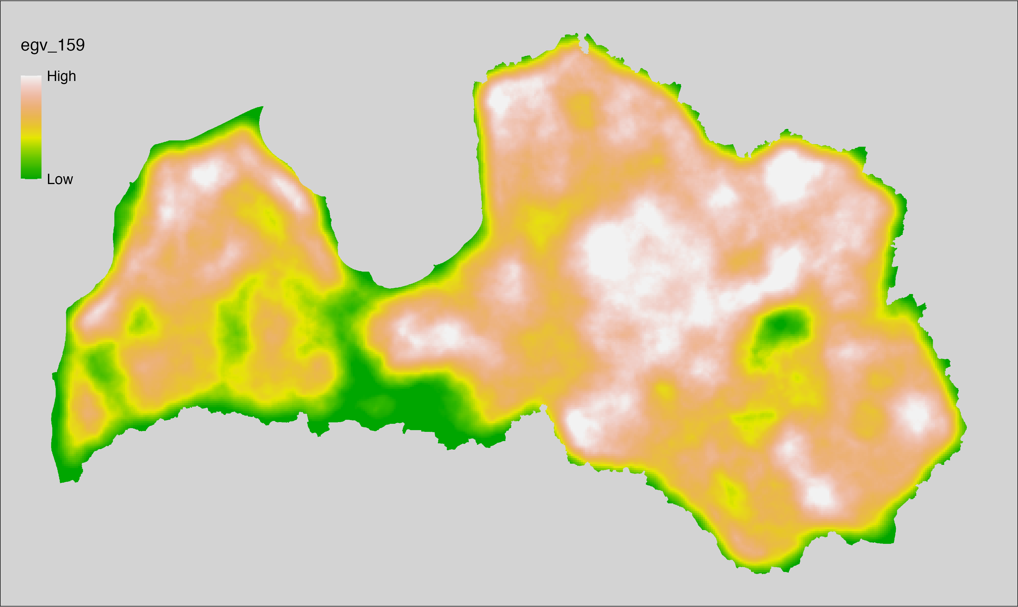
6.160 Edges_Water_cell
filename: Edges_Water_cell.tif
layername: egv_160
English name: Edge pixels of Water within the analysis cell (1 ha)
Latvian name: Ūdenstilpju malu pikseļu skaits analīzes šūnā (1 ha)
Procedure: First, values equal to 200 from the Landscape
classification are coded as 1 and everything else as NA. Then, the
layer (1 = presence) is covered over the nulls layer (presence = 0) and written to
file (matching the input). Next, with the workflow
egvtools::landscape_function() total edge between the two classes is
calculated. During the calculation of the landscape metric, inverse distance weighted
(power = 2) gap filling on the output is applied to ensure no missing values
at the edges. Finally, the layer is standardised by subtracting the arithmetic
mean and dividing by the root mean squared error.
Code
# libs ----
if(!require(terra)) {install.packages("terra"); require(terra)}
if(!require(egvtools)) {remotes::install_github("aavotins/egvtools"); require(egvtools)}
if(!require(sf)) {install.packages("sf"); require(sf)}
if(!require(sfarrow)) {install.packages("sfarrow"); require(sfarrow)}
if(!require(raster)) {install.packages("raster"); require(raster)}
if(!require(fasterize)) {install.packages("fasterize"); require(fasterize)}
if(!require(tidyverse)) {install.packages("tidyverse"); require(tidyverse)}
# Templates -----
template10=rast("./Templates/TemplateRasters/LV10m_10km.tif")
nulls10=rast("./Templates/TemplateRasters/nulls_LV10m_10km.tif")
# simple landscape ----
simple_landscape=rast("./RasterGrids_10m/2024/Ainava_vienk_mask.tif")
# Edges_Water_input.tif ----
water=ifel(simple_landscape==200,1,0)
plot(water)
water=cover(water,nulls10)
plot(water)
edge_water=project(water,template10,
filename="./RasterGrids_10m/2024/Edges_Water_input.tif",
overwrite=TRUE)
# Edges_Water_cell.tif egv_160 ----
landscape_function(
landscape = "./RasterGrids_10m/2024/Edges_Water_input.tif",
zones = "./Templates/TemplateGrids/tikls100_sauzeme.parquet",
id_field = "id",
tile_field = "tks50km",
template = "./Templates/TemplateRasters/LV100m_10km.tif",
out_dir = "./RasterGrids_100m/2024/RAW",
out_filename = "Edges_Water_cell.tif",
out_layername = "egv_160",
what = "lsm_l_te",
lm_args = list(count_boundary = FALSE),
rasterize_engine = "fasterize",
n_workers = 12,
future_max_size = 20 * 1024^3,
fill_gaps = TRUE,
plot_gaps = FALSE,
plot_result = FALSE
)
# standardisation ----
if(!require(terra)) {install.packages("terra"); require(terra)}
if(!require(tidyverse)) {install.packages("tidyverse"); require(tidyverse)}
nosaukums="Edges_Water_cell.tif"
ielasisanas_cels=paste0("./RasterGrids_100m/2024/RAW/",nosaukums)
saglabasanas_cels=paste0("./RasterGrids_100m/2024/Scaled/",nosaukums)
slanis=rast(ielasisanas_cels)
videjais=global(slanis,fun="mean",na.rm=TRUE)
centrets=slanis-videjais[,1]
standartnovirze=terra::global(centrets,fun="rms",na.rm=TRUE)
merogots=centrets/standartnovirze[,1]
writeRaster(merogots,
filename=saglabasanas_cels,
overwrite=TRUE)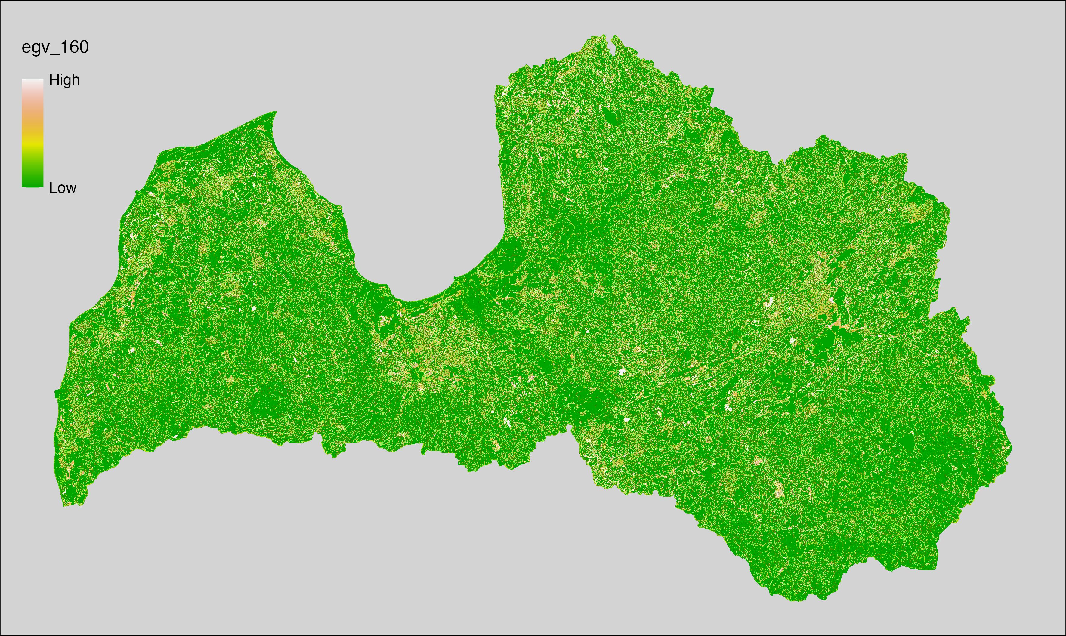
6.161 Edges_Water_r500
filename: Edges_Water_r500.tif
layername: egv_161
English name: Edge pixels of Water within the 0.5 km landscape
Latvian name: Ūdenstilpju malu pikseļu skaits 0,5 km ainavā
Procedure: The total edge within a 500 m radius around the analysis grid cell is
calculated as the area-weighted sum of the analysis cells inside the
buffer, using the workflow egvtools::radius_function(). During the calculation of the landscape metric,
inverse distance weighted (power = 2) gap filling on the output is applied
to ensure no missing values at the edges. Then the layer is rewritten to set
its name. Finally, the layer is standardised by subtracting the arithmetic
mean and dividing by the root mean squared error.
Code
# libs ----
if(!require(terra)) {install.packages("terra"); require(terra)}
if(!require(egvtools)) {remotes::install_github("aavotins/egvtools"); require(egvtools)}
# Templates -----
template100=rast("./Templates/TemplateRasters/LV100m_10km.tif")
# radii ----
radius_function(
kvadrati_path = "./Templates/TemplateGrids/tiles/",
radii_path = "./Templates/TemplateGridPoints/tiles/",
tikls100_path = "./Templates/TemplateGrids/tikls100_sauzeme.parquet",
template_path = "./Templates/TemplateRasters/LV100m_10km.tif",
input_layers = c("./RasterGrids_100m/2024/RAW/Edges_Water_cell.tif"),
layer_prefixes = c("Edges_Water"),
output_dir = "./RasterGrids_100m/2024/RAW/",
n_workers = 12,
radii = c("r500"),
radius_mode = "sparse",
extract_fun = "sum",
fill_missing = TRUE,
IDW_weight = 2,
future_max_size = 20 * 1024^3)
# Edges_Water_r500.tif egv_161 ----
slanis=rast("./RasterGrids_100m/2024/RAW/Edges_Water_r500.tif")
names(slanis)="egv_161"
slanis2=project(slanis,template100)
writeRaster(slanis2,
"./RasterGrids_100m/2024/RAW/Edges_Water_r500.tif",
overwrite=TRUE)
# standardisation ----
if(!require(terra)) {install.packages("terra"); require(terra)}
if(!require(tidyverse)) {install.packages("tidyverse"); require(tidyverse)}
nosaukums="Edges_Water_r500.tif"
ielasisanas_cels=paste0("./RasterGrids_100m/2024/RAW/",nosaukums)
saglabasanas_cels=paste0("./RasterGrids_100m/2024/Scaled/",nosaukums)
slanis=rast(ielasisanas_cels)
videjais=global(slanis,fun="mean",na.rm=TRUE)
centrets=slanis-videjais[,1]
standartnovirze=terra::global(centrets,fun="rms",na.rm=TRUE)
merogots=centrets/standartnovirze[,1]
writeRaster(merogots,
filename=saglabasanas_cels,
overwrite=TRUE)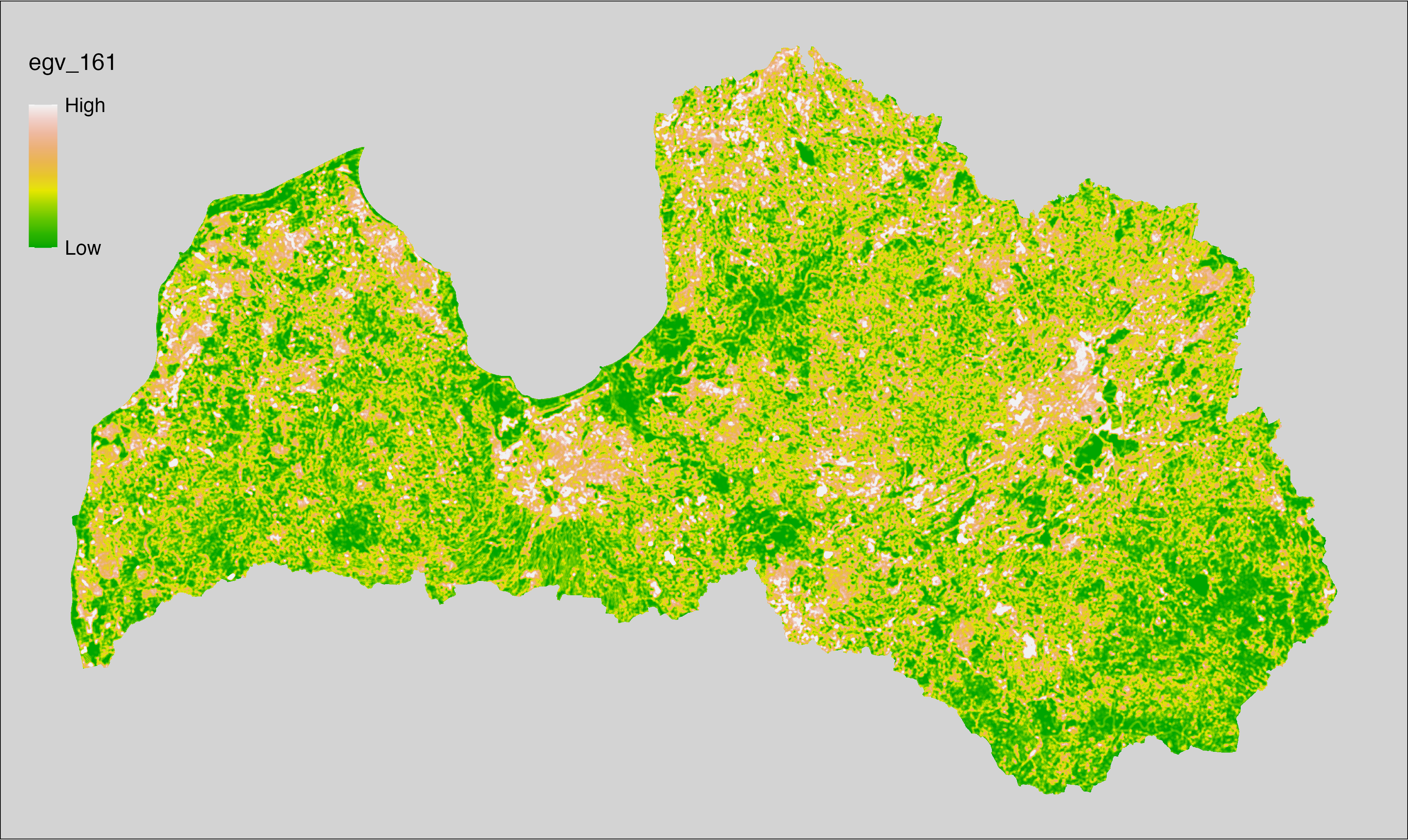
6.162 Edges_Water_r1250
filename: Edges_Water_r1250.tif
layername: egv_162
English name: Edge pixels of Water within the 1.25 km landscape
Latvian name: Ūdenstilpju malu pikseļu skaits 1,25 km ainavā
Procedure: The total edge within a 1250 m radius around the analysis grid cell is
calculated as the area-weighted sum of the analysis cells inside the
buffer, using the workflow egvtools::radius_function(). During the calculation of the landscape metric,
inverse distance weighted (power = 2) gap filling on the output is applied
to ensure no missing values at the edges. Then the layer is rewritten to set
its name. Finally, the layer is standardised by subtracting the arithmetic
mean and dividing by the root mean squared error.
Code
# libs ----
if(!require(terra)) {install.packages("terra"); require(terra)}
if(!require(egvtools)) {remotes::install_github("aavotins/egvtools"); require(egvtools)}
# Templates -----
template100=rast("./Templates/TemplateRasters/LV100m_10km.tif")
# radii ----
radius_function(
kvadrati_path = "./Templates/TemplateGrids/tiles/",
radii_path = "./Templates/TemplateGridPoints/tiles/",
tikls100_path = "./Templates/TemplateGrids/tikls100_sauzeme.parquet",
template_path = "./Templates/TemplateRasters/LV100m_10km.tif",
input_layers = c("./RasterGrids_100m/2024/RAW/Edges_Water_cell.tif"),
layer_prefixes = c("Edges_Water"),
output_dir = "./RasterGrids_100m/2024/RAW/",
n_workers = 12,
radii = c("r1250"),
radius_mode = "sparse",
extract_fun = "sum",
fill_missing = TRUE,
IDW_weight = 2,
future_max_size = 20 * 1024^3)
# Edges_Water_r1250.tif egv_162 ----
slanis=rast("./RasterGrids_100m/2024/RAW/Edges_Water_r1250.tif")
names(slanis)="egv_162"
slanis2=project(slanis,template100)
writeRaster(slanis2,
"./RasterGrids_100m/2024/RAW/Edges_Water_r1250.tif",
overwrite=TRUE)
# standardisation ----
if(!require(terra)) {install.packages("terra"); require(terra)}
if(!require(tidyverse)) {install.packages("tidyverse"); require(tidyverse)}
nosaukums="Edges_Water_r1250.tif"
ielasisanas_cels=paste0("./RasterGrids_100m/2024/RAW/",nosaukums)
saglabasanas_cels=paste0("./RasterGrids_100m/2024/Scaled/",nosaukums)
slanis=rast(ielasisanas_cels)
videjais=global(slanis,fun="mean",na.rm=TRUE)
centrets=slanis-videjais[,1]
standartnovirze=terra::global(centrets,fun="rms",na.rm=TRUE)
merogots=centrets/standartnovirze[,1]
writeRaster(merogots,
filename=saglabasanas_cels,
overwrite=TRUE)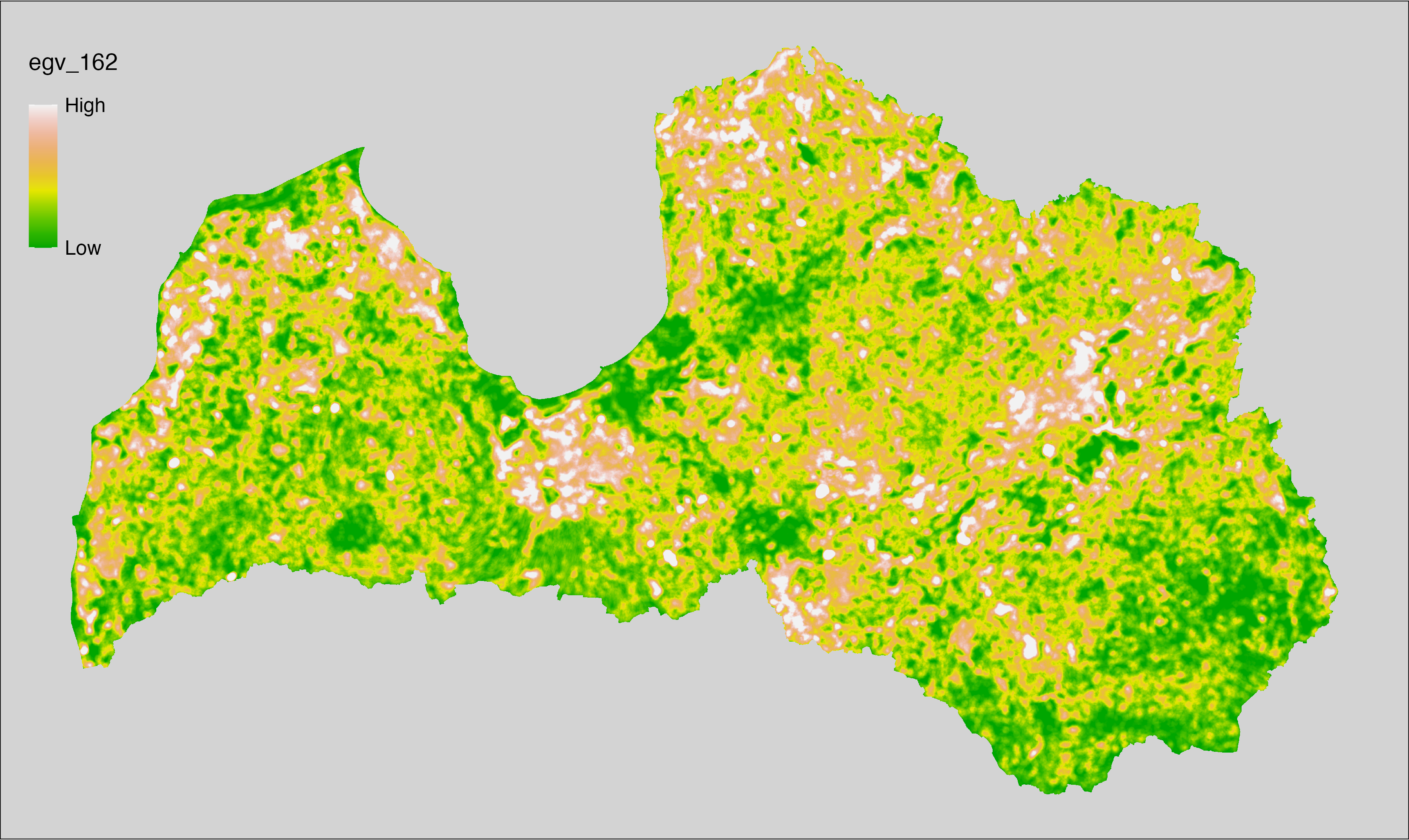
6.163 Edges_Water_r3000
filename: Edges_Water_r3000.tif
layername: egv_163
English name: Edge pixels of Water within the 3 km landscape
Latvian name: Ūdenstilpju malu pikseļu skaits 3 km ainavā
Procedure: The total edge within a 3000 m radius around the analysis grid cell is
calculated as the area-weighted sum of the analysis cells inside the
buffer, using the workflow egvtools::radius_function(). During the calculation of the landscape metric,
inverse distance weighted (power = 2) gap filling on the output is applied
to ensure no missing values at the edges. Then the layer is rewritten to set
its name. Finally, the layer is standardised by subtracting the arithmetic
mean and dividing by the root mean squared error.
Code
# libs ----
if(!require(terra)) {install.packages("terra"); require(terra)}
if(!require(egvtools)) {remotes::install_github("aavotins/egvtools"); require(egvtools)}
# Templates -----
template100=rast("./Templates/TemplateRasters/LV100m_10km.tif")
# radii ----
radius_function(
kvadrati_path = "./Templates/TemplateGrids/tiles/",
radii_path = "./Templates/TemplateGridPoints/tiles/",
tikls100_path = "./Templates/TemplateGrids/tikls100_sauzeme.parquet",
template_path = "./Templates/TemplateRasters/LV100m_10km.tif",
input_layers = c("./RasterGrids_100m/2024/RAW/Edges_Water_cell.tif"),
layer_prefixes = c("Edges_Water"),
output_dir = "./RasterGrids_100m/2024/RAW/",
n_workers = 12,
radii = c("r3000"),
radius_mode = "sparse",
extract_fun = "sum",
fill_missing = TRUE,
IDW_weight = 2,
future_max_size = 20 * 1024^3)
# Edges_Water_r3000.tif egv_163 ----
slanis=rast("./RasterGrids_100m/2024/RAW/Edges_Water_r3000.tif")
names(slanis)="egv_163"
slanis2=project(slanis,template100)
writeRaster(slanis2,
"./RasterGrids_100m/2024/RAW/Edges_Water_r3000.tif",
overwrite=TRUE)
# standardisation ----
if(!require(terra)) {install.packages("terra"); require(terra)}
if(!require(tidyverse)) {install.packages("tidyverse"); require(tidyverse)}
nosaukums="Edges_Water_r3000.tif"
ielasisanas_cels=paste0("./RasterGrids_100m/2024/RAW/",nosaukums)
saglabasanas_cels=paste0("./RasterGrids_100m/2024/Scaled/",nosaukums)
slanis=rast(ielasisanas_cels)
videjais=global(slanis,fun="mean",na.rm=TRUE)
centrets=slanis-videjais[,1]
standartnovirze=terra::global(centrets,fun="rms",na.rm=TRUE)
merogots=centrets/standartnovirze[,1]
writeRaster(merogots,
filename=saglabasanas_cels,
overwrite=TRUE)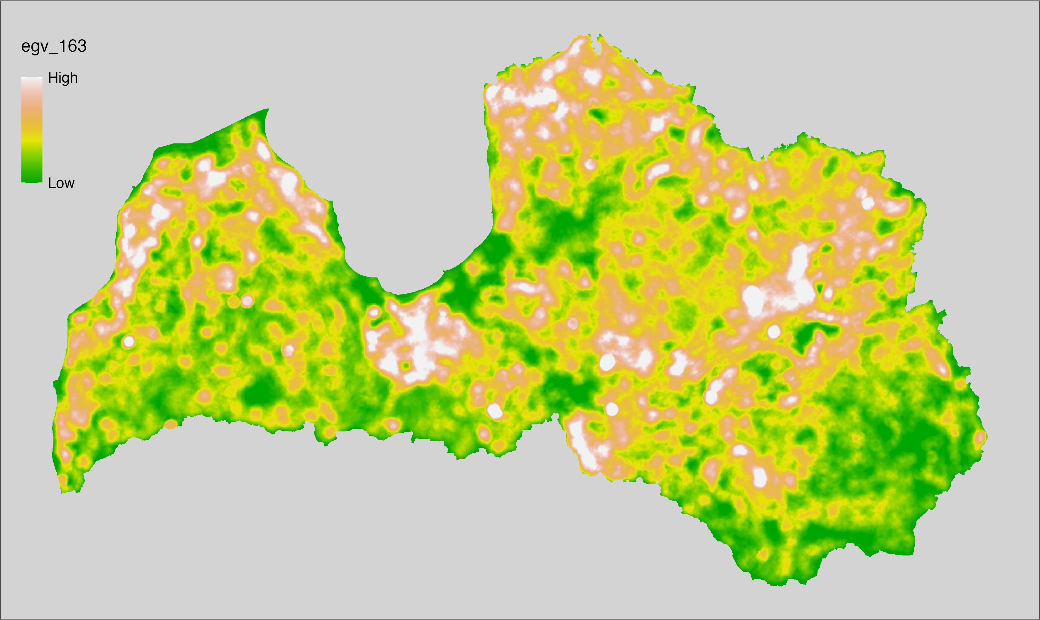
6.164 Edges_Water_r10000
filename: Edges_Water_r10000.tif
layername: egv_164
English name: Edge pixels of Water within the 10 km landscape
Latvian name: Ūdenstilpju malu pikseļu skaits 10 km ainavā
Procedure: The total edge within a 10000 m radius around the analysis grid cell is
calculated as the area-weighted sum of the analysis cells inside the
buffer, using the workflow egvtools::radius_function(). During the calculation of the landscape metric,
inverse distance weighted (power = 2) gap filling on the output is applied
to ensure no missing values at the edges. Then the layer is rewritten to set
its name. Finally, the layer is standardised by subtracting the arithmetic
mean and dividing by the root mean squared error.
Code
# libs ----
if(!require(terra)) {install.packages("terra"); require(terra)}
if(!require(egvtools)) {remotes::install_github("aavotins/egvtools"); require(egvtools)}
# Templates -----
template100=rast("./Templates/TemplateRasters/LV100m_10km.tif")
# radii ----
radius_function(
kvadrati_path = "./Templates/TemplateGrids/tiles/",
radii_path = "./Templates/TemplateGridPoints/tiles/",
tikls100_path = "./Templates/TemplateGrids/tikls100_sauzeme.parquet",
template_path = "./Templates/TemplateRasters/LV100m_10km.tif",
input_layers = c("./RasterGrids_100m/2024/RAW/Edges_Water_cell.tif"),
layer_prefixes = c("Edges_Water"),
output_dir = "./RasterGrids_100m/2024/RAW/",
n_workers = 12,
radii = c("r10000"),
radius_mode = "sparse",
extract_fun = "sum",
fill_missing = TRUE,
IDW_weight = 2,
future_max_size = 20 * 1024^3)
# Edges_Water_r10000.tif egv_164 ----
slanis=rast("./RasterGrids_100m/2024/RAW/Edges_Water_r10000.tif")
names(slanis)="egv_164"
slanis2=project(slanis,template100)
writeRaster(slanis2,
"./RasterGrids_100m/2024/RAW/Edges_Water_r10000.tif",
overwrite=TRUE)
# standardisation ----
if(!require(terra)) {install.packages("terra"); require(terra)}
if(!require(tidyverse)) {install.packages("tidyverse"); require(tidyverse)}
nosaukums="Edges_Water_r10000.tif"
ielasisanas_cels=paste0("./RasterGrids_100m/2024/RAW/",nosaukums)
saglabasanas_cels=paste0("./RasterGrids_100m/2024/Scaled/",nosaukums)
slanis=rast(ielasisanas_cels)
videjais=global(slanis,fun="mean",na.rm=TRUE)
centrets=slanis-videjais[,1]
standartnovirze=terra::global(centrets,fun="rms",na.rm=TRUE)
merogots=centrets/standartnovirze[,1]
writeRaster(merogots,
filename=saglabasanas_cels,
overwrite=TRUE)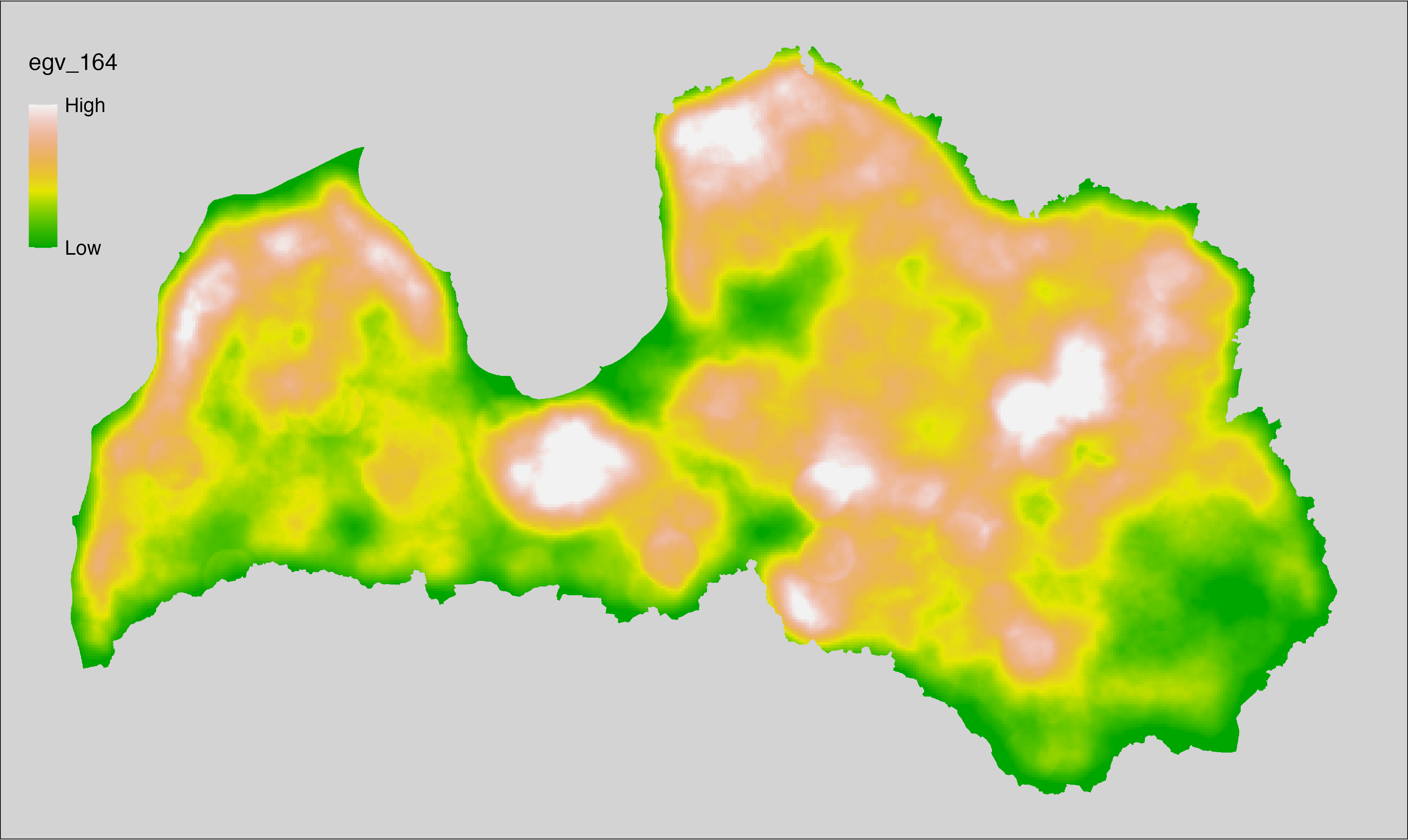
6.165 Edges_Water-Farmland_cell
filename: Edges_Water-Farmland_cell.tif
layername: egv_165
English name: Edge pixels of Water bordering with Farmland within the analysis cell (1 ha)
Latvian name: Ūdenstilpju malu ar lauksaimniecības zemēm pikseļu skaits analīzes šūnā (1 ha)
Procedure: First, values larger than 300 and smaller than 400 from
Landscape classification are coded as 1, and all other values as NA.
Then values equal to 200 from the Landscape classification are coded as
0, and all other values as NA. Then, the first layer (1 = presence) is covered over
the second layer (presence = 0) and written to file (matching the input). Next,
using the workflow egvtools::landscape_function() total edge between the two
classes is calculated. During the calculation of the landscape metric, inverse distance
weighted (power = 2) gap filling on the output is applied to ensure no
missing values at the edges. Finally, the layer is standardised by
subtracting the arithmetic mean and dividing by the root mean squared error.
Code
# libs ----
if(!require(terra)) {install.packages("terra"); require(terra)}
if(!require(egvtools)) {remotes::install_github("aavotins/egvtools"); require(egvtools)}
if(!require(sf)) {install.packages("sf"); require(sf)}
if(!require(sfarrow)) {install.packages("sfarrow"); require(sfarrow)}
if(!require(raster)) {install.packages("raster"); require(raster)}
if(!require(fasterize)) {install.packages("fasterize"); require(fasterize)}
if(!require(tidyverse)) {install.packages("tidyverse"); require(tidyverse)}
# Templates -----
template10=rast("./Templates/TemplateRasters/LV10m_10km.tif")
nulls10=rast("./Templates/TemplateRasters/nulls_LV10m_10km.tif")
# simple landscape ----
simple_landscape=rast("./RasterGrids_10m/2024/Ainava_vienk_mask.tif")
# Edges_Water-Farmland_input.tif ----
water=ifel(simple_landscape==200,0,NA)
plot(water)
farmland=ifel(simple_landscape>300 & simple_landscape<400,1,NA)
plot(farmland)
water_farmland=cover(water,farmland)
plot(water_farmland)
edge_water_farmland=project(water_farmland,template10,
filename="./RasterGrids_10m/2024/Edges_Water-Farmland_input.tif",
overwrite=TRUE)
rm(edge_water_farmland)
rm(water_farmland)
# Edges_Water-Farmland_cell.tif egv_165 ----
landscape_function(
landscape = "./RasterGrids_10m/2024/Edges_Water-Farmland_input.tif",
zones = "./Templates/TemplateGrids/tikls100_sauzeme.parquet",
id_field = "id",
tile_field = "tks50km",
template = "./Templates/TemplateRasters/LV100m_10km.tif",
out_dir = "./RasterGrids_100m/2024/RAW",
out_filename = "Edges_Water-Farmland_cell.tif",
out_layername = "egv_165",
what = "lsm_l_te",
lm_args = list(count_boundary = FALSE),
rasterize_engine = "fasterize",
n_workers = 12,
future_max_size = 20 * 1024^3,
fill_gaps = TRUE,
plot_gaps = FALSE,
plot_result = FALSE
)
# standardisation ----
if(!require(terra)) {install.packages("terra"); require(terra)}
if(!require(tidyverse)) {install.packages("tidyverse"); require(tidyverse)}
nosaukums="Edges_Water-Farmland_cell.tif"
ielasisanas_cels=paste0("./RasterGrids_100m/2024/RAW/",nosaukums)
saglabasanas_cels=paste0("./RasterGrids_100m/2024/Scaled/",nosaukums)
slanis=rast(ielasisanas_cels)
videjais=global(slanis,fun="mean",na.rm=TRUE)
centrets=slanis-videjais[,1]
standartnovirze=terra::global(centrets,fun="rms",na.rm=TRUE)
merogots=centrets/standartnovirze[,1]
writeRaster(merogots,
filename=saglabasanas_cels,
overwrite=TRUE)
6.166 Edges_Water-Farmland_r500
filename: Edges_Water-Farmland_r500.tif
layername: egv_166
English name: Edge pixels of Water bordering with Farmland within the 0.5 km landscape
Latvian name: Ūdenstilpju malu ar lauksaimniecības zemēm pikseļu skaits 0,5 km ainavā
Procedure: The total edge within a 500 m radius around the analysis grid cell is
calculated as the area-weighted sum of the analysis cells inside the
buffer, using the workflow egvtools::radius_function(). During the calculation of the landscape metric,
inverse distance weighted (power = 2) gap filling on the output is applied
to ensure no missing values at the edges. Then the layer is rewritten to set
its name. Finally, the layer is standardised by subtracting the arithmetic
mean and dividing by the root mean squared error.
Code
# libs ----
if(!require(terra)) {install.packages("terra"); require(terra)}
if(!require(egvtools)) {remotes::install_github("aavotins/egvtools"); require(egvtools)}
# Templates -----
template100=rast("./Templates/TemplateRasters/LV100m_10km.tif")
# radii ----
radius_function(
kvadrati_path = "./Templates/TemplateGrids/tiles/",
radii_path = "./Templates/TemplateGridPoints/tiles/",
tikls100_path = "./Templates/TemplateGrids/tikls100_sauzeme.parquet",
template_path = "./Templates/TemplateRasters/LV100m_10km.tif",
input_layers = c("./RasterGrids_100m/2024/RAW/Edges_Water-Farmland_cell.tif"),
layer_prefixes = c("Edges_Water-Farmland"),
output_dir = "./RasterGrids_100m/2024/RAW/",
n_workers = 12,
radii = c("r500"),
radius_mode = "sparse",
extract_fun = "sum",
fill_missing = TRUE,
IDW_weight = 2,
future_max_size = 20 * 1024^3)
# Edges_Water-Farmland_r500.tif egv_166 -----
slanis=rast("./RasterGrids_100m/2024/RAW/Edges_Water-Farmland_r500.tif")
names(slanis)="egv_166"
slanis2=project(slanis,template100)
writeRaster(slanis2,
"./RasterGrids_100m/2024/RAW/Edges_Water-Farmland_r500.tif",
overwrite=TRUE)
# standardisation ----
if(!require(terra)) {install.packages("terra"); require(terra)}
if(!require(tidyverse)) {install.packages("tidyverse"); require(tidyverse)}
nosaukums="Edges_Water-Farmland_r500.tif"
ielasisanas_cels=paste0("./RasterGrids_100m/2024/RAW/",nosaukums)
saglabasanas_cels=paste0("./RasterGrids_100m/2024/Scaled/",nosaukums)
slanis=rast(ielasisanas_cels)
videjais=global(slanis,fun="mean",na.rm=TRUE)
centrets=slanis-videjais[,1]
standartnovirze=terra::global(centrets,fun="rms",na.rm=TRUE)
merogots=centrets/standartnovirze[,1]
writeRaster(merogots,
filename=saglabasanas_cels,
overwrite=TRUE)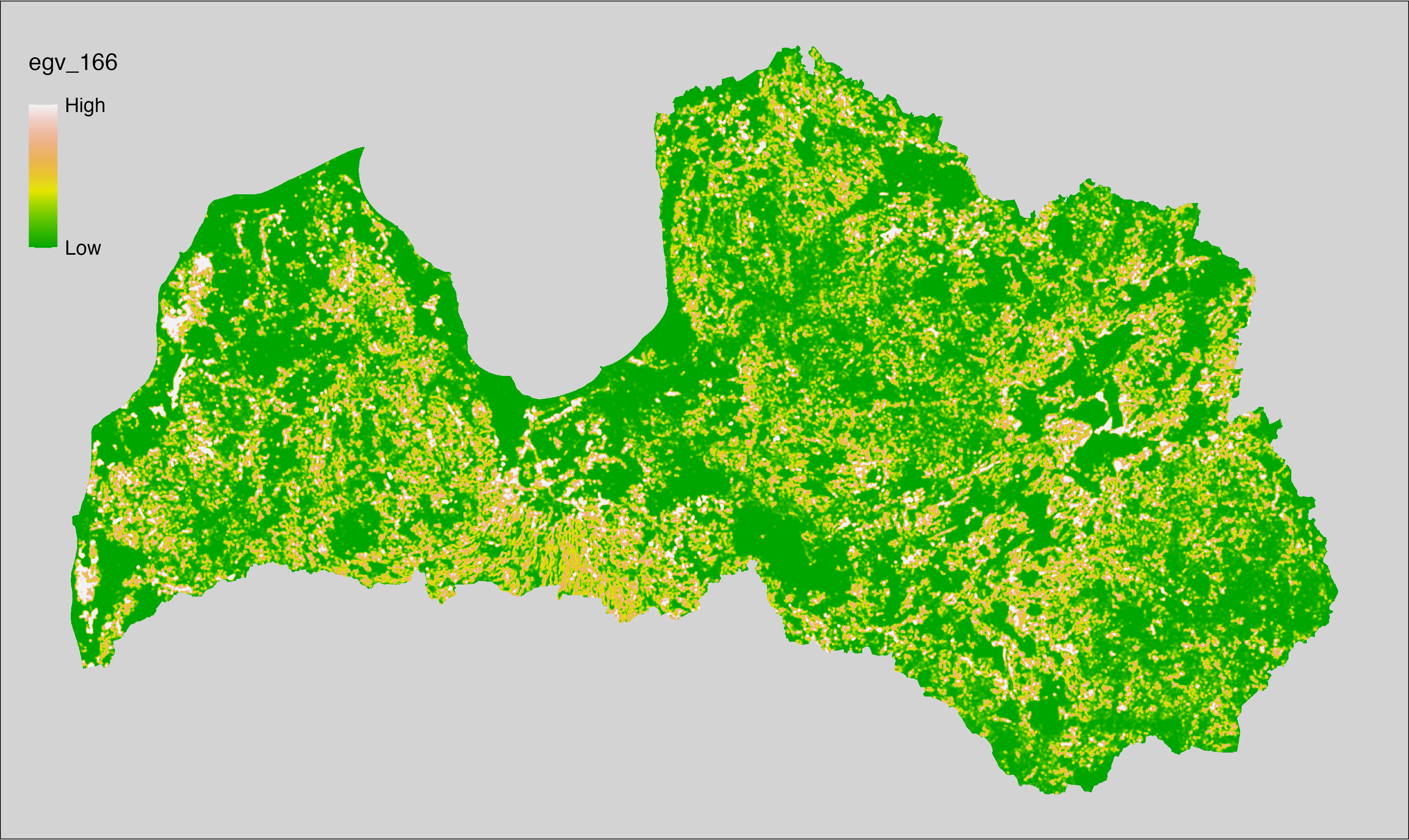
6.167 Edges_Water-Farmland_r1250
filename: Edges_Water-Farmland_r1250.tif
layername: egv_167
English name: Edge pixels of Water bordering with Farmland within the 1.25 km landscape
Latvian name: Ūdenstilpju malu ar lauksaimniecības zemēm pikseļu skaits 1,25 km ainavā
Procedure: The total edge within a 1250 m radius around the analysis grid cell is
calculated as the area-weighted sum of the analysis cells inside the
buffer, using the workflow egvtools::radius_function(). During the calculation of the landscape metric,
inverse distance weighted (power = 2) gap filling on the output is applied
to ensure no missing values at the edges. Then the layer is rewritten to set
its name. Finally, the layer is standardised by subtracting the arithmetic
mean and dividing by the root mean squared error.
Code
# libs ----
if(!require(terra)) {install.packages("terra"); require(terra)}
if(!require(egvtools)) {remotes::install_github("aavotins/egvtools"); require(egvtools)}
# Templates -----
template100=rast("./Templates/TemplateRasters/LV100m_10km.tif")
# radii ----
radius_function(
kvadrati_path = "./Templates/TemplateGrids/tiles/",
radii_path = "./Templates/TemplateGridPoints/tiles/",
tikls100_path = "./Templates/TemplateGrids/tikls100_sauzeme.parquet",
template_path = "./Templates/TemplateRasters/LV100m_10km.tif",
input_layers = c("./RasterGrids_100m/2024/RAW/Edges_Water-Farmland_cell.tif"),
layer_prefixes = c("Edges_Water-Farmland"),
output_dir = "./RasterGrids_100m/2024/RAW/",
n_workers = 12,
radii = c("r1250"),
radius_mode = "sparse",
extract_fun = "sum",
fill_missing = TRUE,
IDW_weight = 2,
future_max_size = 20 * 1024^3)
# Edges_Water-Farmland_r1250.tif egv_167 ----
slanis=rast("./RasterGrids_100m/2024/RAW/Edges_Water-Farmland_r1250.tif")
names(slanis)="egv_167"
slanis2=project(slanis,template100)
writeRaster(slanis2,
"./RasterGrids_100m/2024/RAW/Edges_Water-Farmland_r1250.tif",
overwrite=TRUE)
# standardisation ----
if(!require(terra)) {install.packages("terra"); require(terra)}
if(!require(tidyverse)) {install.packages("tidyverse"); require(tidyverse)}
nosaukums="Edges_Water-Farmland_r1250.tif"
ielasisanas_cels=paste0("./RasterGrids_100m/2024/RAW/",nosaukums)
saglabasanas_cels=paste0("./RasterGrids_100m/2024/Scaled/",nosaukums)
slanis=rast(ielasisanas_cels)
videjais=global(slanis,fun="mean",na.rm=TRUE)
centrets=slanis-videjais[,1]
standartnovirze=terra::global(centrets,fun="rms",na.rm=TRUE)
merogots=centrets/standartnovirze[,1]
writeRaster(merogots,
filename=saglabasanas_cels,
overwrite=TRUE)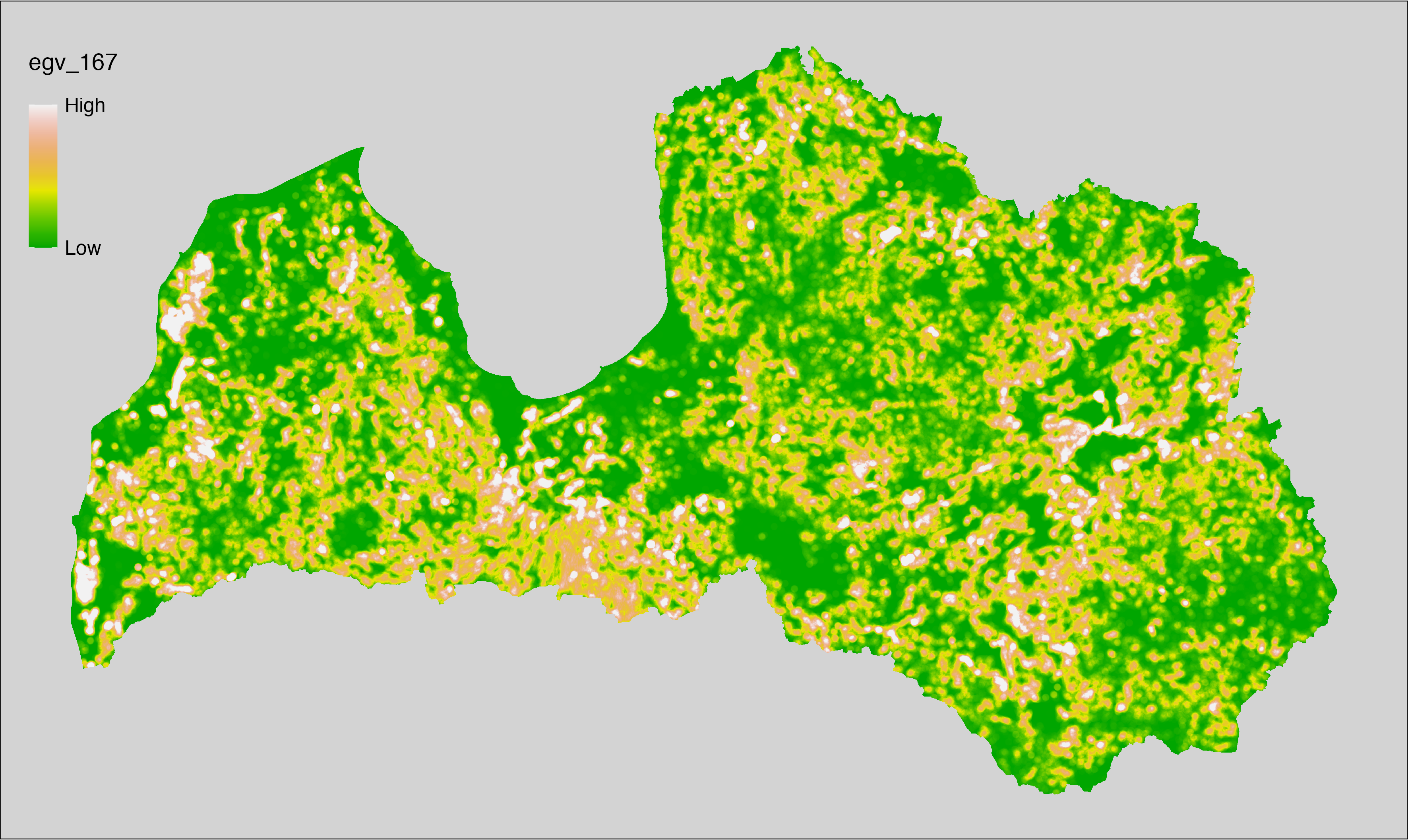
6.168 Edges_Water-Farmland_r3000
filename: Edges_Water-Farmland_r3000.tif
layername: egv_168
English name: Edge pixels of Water bordering with Farmland within the 3 km landscape
Latvian name: Ūdenstilpju malu ar lauksaimniecības zemēm pikseļu skaits 3 km ainavā
Procedure: The total edge within a 3000 m radius around the analysis grid cell is
calculated as the area-weighted sum of the analysis cells inside the
buffer, using the workflow egvtools::radius_function(). During the calculation of the landscape metric,
inverse distance weighted (power = 2) gap filling on the output is applied
to ensure no missing values at the edges. Then the layer is rewritten to set
its name. Finally, the layer is standardised by subtracting the arithmetic
mean and dividing by the root mean squared error.
Code
# libs ----
if(!require(terra)) {install.packages("terra"); require(terra)}
if(!require(egvtools)) {remotes::install_github("aavotins/egvtools"); require(egvtools)}
# Templates -----
template100=rast("./Templates/TemplateRasters/LV100m_10km.tif")
# radii ----
radius_function(
kvadrati_path = "./Templates/TemplateGrids/tiles/",
radii_path = "./Templates/TemplateGridPoints/tiles/",
tikls100_path = "./Templates/TemplateGrids/tikls100_sauzeme.parquet",
template_path = "./Templates/TemplateRasters/LV100m_10km.tif",
input_layers = c("./RasterGrids_100m/2024/RAW/Edges_Water-Farmland_cell.tif"),
layer_prefixes = c("Edges_Water-Farmland"),
output_dir = "./RasterGrids_100m/2024/RAW/",
n_workers = 12,
radii = c("r3000"),
radius_mode = "sparse",
extract_fun = "sum",
fill_missing = TRUE,
IDW_weight = 2,
future_max_size = 20 * 1024^3)
# Edges_Water-Farmland_r3000.tif egv_168 ----
slanis=rast("./RasterGrids_100m/2024/RAW/Edges_Water-Farmland_r3000.tif")
names(slanis)="egv_168"
slanis2=project(slanis,template100)
writeRaster(slanis2,
"./RasterGrids_100m/2024/RAW/Edges_Water-Farmland_r3000.tif",
overwrite=TRUE)
# standardisation ----
if(!require(terra)) {install.packages("terra"); require(terra)}
if(!require(tidyverse)) {install.packages("tidyverse"); require(tidyverse)}
nosaukums="Edges_Water-Farmland_r3000.tif"
ielasisanas_cels=paste0("./RasterGrids_100m/2024/RAW/",nosaukums)
saglabasanas_cels=paste0("./RasterGrids_100m/2024/Scaled/",nosaukums)
slanis=rast(ielasisanas_cels)
videjais=global(slanis,fun="mean",na.rm=TRUE)
centrets=slanis-videjais[,1]
standartnovirze=terra::global(centrets,fun="rms",na.rm=TRUE)
merogots=centrets/standartnovirze[,1]
writeRaster(merogots,
filename=saglabasanas_cels,
overwrite=TRUE)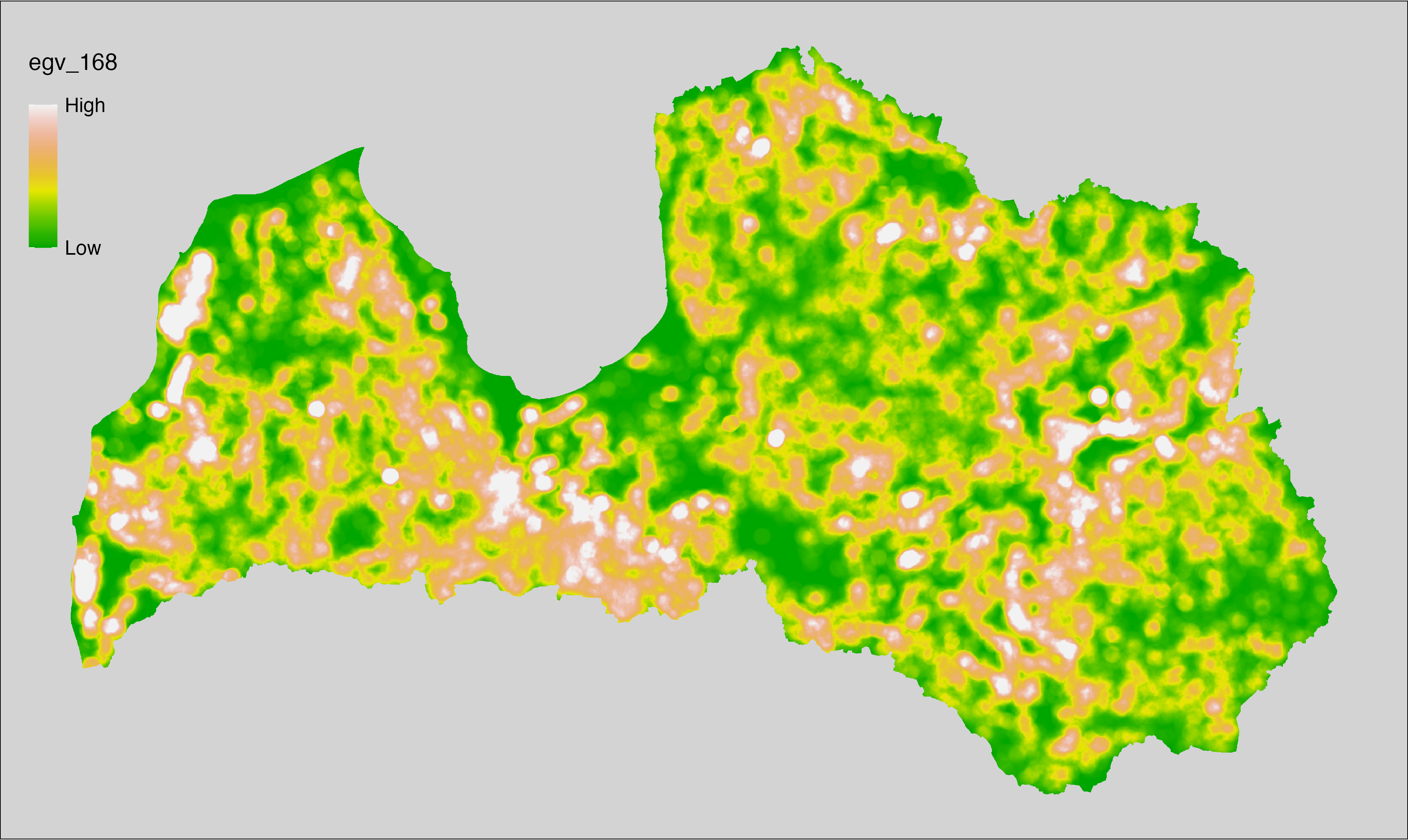
6.169 Edges_Water-Farmland_r10000
filename: Edges_Water-Farmland_r10000.tif
layername: egv_169
English name: Edge pixels of Water bordering with Farmland within the 10 km landscape
Latvian name: Ūdenstilpju malu ar lauksaimniecības zemēm pikseļu skaits 10 km ainavā
Procedure: The total edge within a 10000 m radius around the analysis grid cell is
calculated as the area-weighted sum of the analysis cells inside the
buffer, using the workflow egvtools::radius_function(). During the calculation of the landscape metric,
inverse distance weighted (power = 2) gap filling on the output is applied
to ensure no missing values at the edges. Then the layer is rewritten to set
its name. Finally, the layer is standardised by subtracting the arithmetic
mean and dividing by the root mean squared error.
Code
# libs ----
if(!require(terra)) {install.packages("terra"); require(terra)}
if(!require(egvtools)) {remotes::install_github("aavotins/egvtools"); require(egvtools)}
# Templates -----
template100=rast("./Templates/TemplateRasters/LV100m_10km.tif")
# radii ----
radius_function(
kvadrati_path = "./Templates/TemplateGrids/tiles/",
radii_path = "./Templates/TemplateGridPoints/tiles/",
tikls100_path = "./Templates/TemplateGrids/tikls100_sauzeme.parquet",
template_path = "./Templates/TemplateRasters/LV100m_10km.tif",
input_layers = c("./RasterGrids_100m/2024/RAW/Edges_Water-Farmland_cell.tif"),
layer_prefixes = c("Edges_Water-Farmland"),
output_dir = "./RasterGrids_100m/2024/RAW/",
n_workers = 12,
radii = c("r3000"),
radius_mode = "sparse",
extract_fun = "sum",
fill_missing = TRUE,
IDW_weight = 2,
future_max_size = 20 * 1024^3)
# Edges_Water-Farmland_r10000.tif egv_169 ----
slanis=rast("./RasterGrids_100m/2024/RAW/Edges_Water-Farmland_r10000.tif")
names(slanis)="egv_169"
slanis2=project(slanis,template100)
writeRaster(slanis2,
"./RasterGrids_100m/2024/RAW/Edges_Water-Farmland_r10000.tif",
overwrite=TRUE)
# standardisation ----
if(!require(terra)) {install.packages("terra"); require(terra)}
if(!require(tidyverse)) {install.packages("tidyverse"); require(tidyverse)}
nosaukums="Edges_Water-Farmland_r10000.tif"
ielasisanas_cels=paste0("./RasterGrids_100m/2024/RAW/",nosaukums)
saglabasanas_cels=paste0("./RasterGrids_100m/2024/Scaled/",nosaukums)
slanis=rast(ielasisanas_cels)
videjais=global(slanis,fun="mean",na.rm=TRUE)
centrets=slanis-videjais[,1]
standartnovirze=terra::global(centrets,fun="rms",na.rm=TRUE)
merogots=centrets/standartnovirze[,1]
writeRaster(merogots,
filename=saglabasanas_cels,
overwrite=TRUE)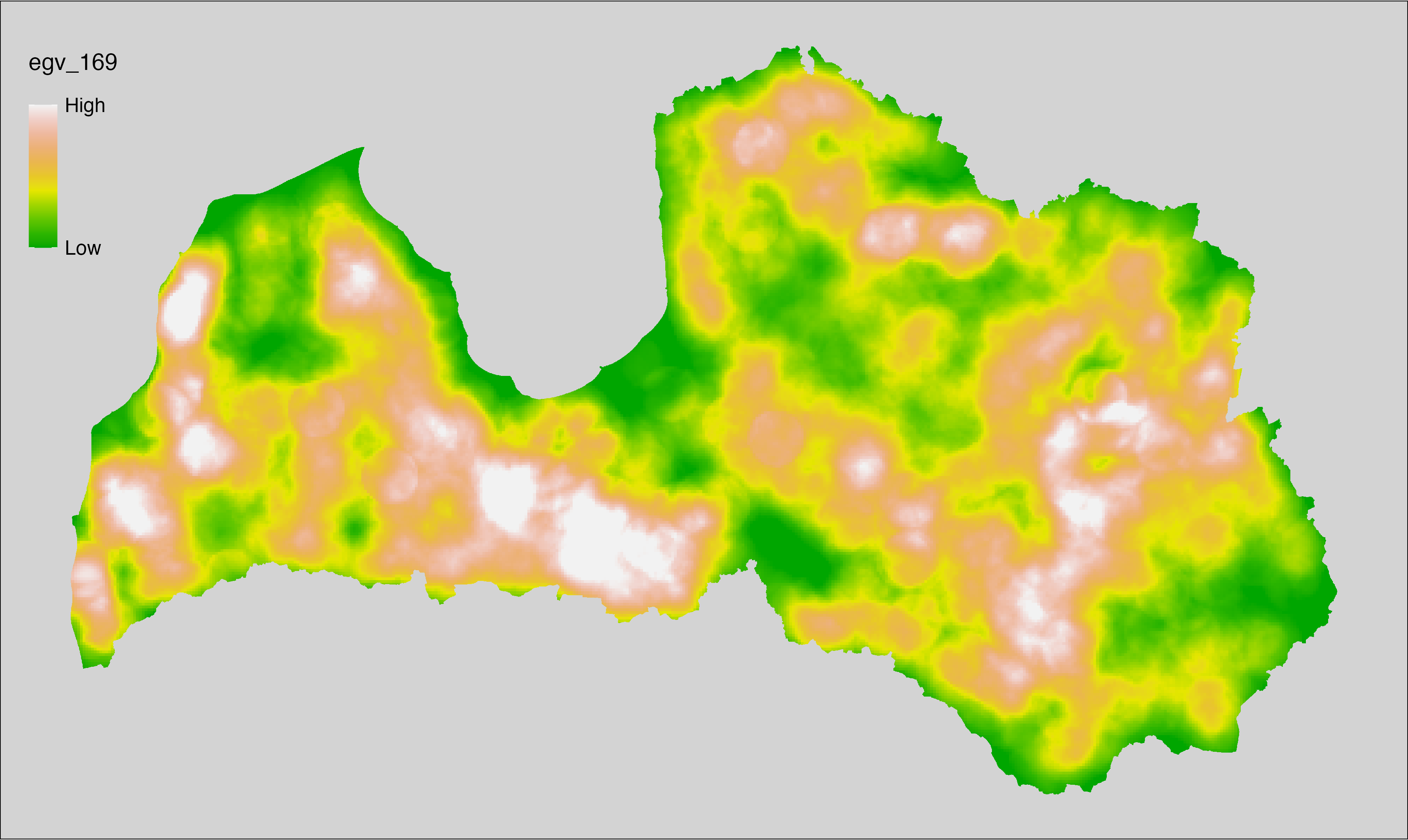
6.170 Edges_Water-Grassland_cell
filename: Edges_Water-Grassland_cell.tif
layername: egv_170
English name: Edge pixels of Water bordering with Grassland within the analysis cell (1 ha)
Latvian name: Ūdenstilpju malu ar zālājiem pikseļu skaits analīzes šūnā (1 ha)
Procedure: First, values lequal to 330 from the Landscape
classification are coded as 1, and all other values as NA. Then values
equal to 200 from the Landscape classification are coded as 0, and
all other values as NA. Then, the first layer (1 = presence) is covered over the
second layer (presence = 0) and written to file (matching the input). Next,
with the workflow egvtools::landscape_function() total edge between the two
classes is calculated. During the calculation of the landscape metric, inverse distance
weighted (power = 2) gap filling on the output is applied to ensure no
missing values at the edges. Finally, the layer is standardised by
subtracting the arithmetic mean and dividing by the root mean squared error.
Code
# libs ----
if(!require(terra)) {install.packages("terra"); require(terra)}
if(!require(egvtools)) {remotes::install_github("aavotins/egvtools"); require(egvtools)}
if(!require(sf)) {install.packages("sf"); require(sf)}
if(!require(sfarrow)) {install.packages("sfarrow"); require(sfarrow)}
if(!require(raster)) {install.packages("raster"); require(raster)}
if(!require(fasterize)) {install.packages("fasterize"); require(fasterize)}
if(!require(tidyverse)) {install.packages("tidyverse"); require(tidyverse)}
# Templates -----
template10=rast("./Templates/TemplateRasters/LV10m_10km.tif")
nulls10=rast("./Templates/TemplateRasters/nulls_LV10m_10km.tif")
# simple landscape ----
simple_landscape=rast("./RasterGrids_10m/2024/Ainava_vienk_mask.tif")
# Edges_Water-Grassland_input.tif ----
water=ifel(simple_landscape==200,0,NA)
plot(water)
grassland=ifel(simple_landscape==330,1,NA)
plot(grassland)
water_grassland=cover(water,grassland)
plot(water_grassland)
edge_water_grassland=project(water_grassland,template10,
filename="./RasterGrids_10m/2024/Edges_Water-Grassland_input.tif",
overwrite=TRUE)
rm(edge_water_grassland)
rm(water_grassland)
# Edges_Water-Grassland_cell.tif egv_170 ----
landscape_function(
landscape = "./RasterGrids_10m/2024/Edges_Water-Grassland_input.tif",
zones = "./Templates/TemplateGrids/tikls100_sauzeme.parquet",
id_field = "id",
tile_field = "tks50km",
template = "./Templates/TemplateRasters/LV100m_10km.tif",
out_dir = "./RasterGrids_100m/2024/RAW",
out_filename = "Edges_Water-Grassland_cell.tif",
out_layername = "egv_170",
what = "lsm_l_te",
lm_args = list(count_boundary = FALSE),
rasterize_engine = "fasterize",
n_workers = 12,
future_max_size = 20 * 1024^3,
fill_gaps = TRUE,
plot_gaps = FALSE,
plot_result = FALSE
)
# standardisation ----
if(!require(terra)) {install.packages("terra"); require(terra)}
if(!require(tidyverse)) {install.packages("tidyverse"); require(tidyverse)}
nosaukums="Edges_Water-Grassland_cell.tif"
ielasisanas_cels=paste0("./RasterGrids_100m/2024/RAW/",nosaukums)
saglabasanas_cels=paste0("./RasterGrids_100m/2024/Scaled/",nosaukums)
slanis=rast(ielasisanas_cels)
videjais=global(slanis,fun="mean",na.rm=TRUE)
centrets=slanis-videjais[,1]
standartnovirze=terra::global(centrets,fun="rms",na.rm=TRUE)
merogots=centrets/standartnovirze[,1]
writeRaster(merogots,
filename=saglabasanas_cels,
overwrite=TRUE)
6.171 Edges_Water-Grassland_r500
filename: Edges_Water-Grassland_r500.tif
layername: egv_171
English name: Edge pixels of Water bordering with Grassland within the 0.5 km landscape
Latvian name: Ūdenstilpju malu ar zālājiem pikseļu skaits 0,5 km ainavā
Procedure: The total edge within a 500 m radius around the analysis grid cell is
calculated as the area-weighted sum of the analysis cells inside the
buffer, using the workflow egvtools::radius_function(). During the calculation of the landscape metric,
inverse distance weighted (power = 2) gap filling on the output is applied
to ensure no missing values at the edges. Then the layer is rewritten to set
its name. Finally, the layer is standardised by subtracting the arithmetic
mean and dividing by the root mean squared error.
Code
# libs ----
if(!require(terra)) {install.packages("terra"); require(terra)}
if(!require(egvtools)) {remotes::install_github("aavotins/egvtools"); require(egvtools)}
# Templates -----
template100=rast("./Templates/TemplateRasters/LV100m_10km.tif")
# radii ----
radius_function(
kvadrati_path = "./Templates/TemplateGrids/tiles/",
radii_path = "./Templates/TemplateGridPoints/tiles/",
tikls100_path = "./Templates/TemplateGrids/tikls100_sauzeme.parquet",
template_path = "./Templates/TemplateRasters/LV100m_10km.tif",
input_layers = c("./RasterGrids_100m/2024/RAW/Edges_Water-Grassland_cell.tif"),
layer_prefixes = c("Edges_Water-Grassland"),
output_dir = "./RasterGrids_100m/2024/RAW/",
n_workers = 12,
radii = c("r500"),
radius_mode = "sparse",
extract_fun = "sum",
fill_missing = TRUE,
IDW_weight = 2,
future_max_size = 20 * 1024^3)
# Edges_Water-Grassland_r500.tif egv_171 ----
slanis=rast("./RasterGrids_100m/2024/RAW/Edges_Water-Grassland_r500.tif")
names(slanis)="egv_171"
slanis2=project(slanis,template100)
writeRaster(slanis2,
"./RasterGrids_100m/2024/RAW/Edges_Water-Grassland_r500.tif",
overwrite=TRUE)
# standardisation ----
if(!require(terra)) {install.packages("terra"); require(terra)}
if(!require(tidyverse)) {install.packages("tidyverse"); require(tidyverse)}
nosaukums="Edges_Water-Grassland_r500.tif"
ielasisanas_cels=paste0("./RasterGrids_100m/2024/RAW/",nosaukums)
saglabasanas_cels=paste0("./RasterGrids_100m/2024/Scaled/",nosaukums)
slanis=rast(ielasisanas_cels)
videjais=global(slanis,fun="mean",na.rm=TRUE)
centrets=slanis-videjais[,1]
standartnovirze=terra::global(centrets,fun="rms",na.rm=TRUE)
merogots=centrets/standartnovirze[,1]
writeRaster(merogots,
filename=saglabasanas_cels,
overwrite=TRUE)
6.172 Edges_Water-Grassland_r1250
filename: Edges_Water-Grassland_r1250.tif
layername: egv_172
English name: Edge pixels of Water bordering with Grassland within the 1.25 km landscape
Latvian name: Ūdenstilpju malu ar zālājiem pikseļu skaits 1,25 km ainavā
Procedure: The total edge within a 1250 m radius around the analysis grid cell is
calculated as the area-weighted sum of the analysis cells inside the
buffer, using the workflow egvtools::radius_function(). During the calculation of the landscape metric,
inverse distance weighted (power = 2) gap filling on the output is applied
to ensure no missing values at the edges. Then the layer is rewritten to set
its name. Finally, the layer is standardised by subtracting the arithmetic
mean and dividing by the root mean squared error.
Code
# libs ----
if(!require(terra)) {install.packages("terra"); require(terra)}
if(!require(egvtools)) {remotes::install_github("aavotins/egvtools"); require(egvtools)}
# Templates -----
template100=rast("./Templates/TemplateRasters/LV100m_10km.tif")
# radii ----
radius_function(
kvadrati_path = "./Templates/TemplateGrids/tiles/",
radii_path = "./Templates/TemplateGridPoints/tiles/",
tikls100_path = "./Templates/TemplateGrids/tikls100_sauzeme.parquet",
template_path = "./Templates/TemplateRasters/LV100m_10km.tif",
input_layers = c("./RasterGrids_100m/2024/RAW/Edges_Water-Grassland_cell.tif"),
layer_prefixes = c("Edges_Water-Grassland"),
output_dir = "./RasterGrids_100m/2024/RAW/",
n_workers = 12,
radii = c("r1250"),
radius_mode = "sparse",
extract_fun = "sum",
fill_missing = TRUE,
IDW_weight = 2,
future_max_size = 20 * 1024^3)
# Edges_Water-Grassland_r1250.tif egv_172 ----
slanis=rast("./RasterGrids_100m/2024/RAW/Edges_Water-Grassland_r1250.tif")
names(slanis)="egv_172"
slanis2=project(slanis,template100)
writeRaster(slanis2,
"./RasterGrids_100m/2024/RAW/Edges_Water-Grassland_r1250.tif",
overwrite=TRUE)
# standardisation ----
if(!require(terra)) {install.packages("terra"); require(terra)}
if(!require(tidyverse)) {install.packages("tidyverse"); require(tidyverse)}
nosaukums="Edges_Water-Grassland_r1250.tif"
ielasisanas_cels=paste0("./RasterGrids_100m/2024/RAW/",nosaukums)
saglabasanas_cels=paste0("./RasterGrids_100m/2024/Scaled/",nosaukums)
slanis=rast(ielasisanas_cels)
videjais=global(slanis,fun="mean",na.rm=TRUE)
centrets=slanis-videjais[,1]
standartnovirze=terra::global(centrets,fun="rms",na.rm=TRUE)
merogots=centrets/standartnovirze[,1]
writeRaster(merogots,
filename=saglabasanas_cels,
overwrite=TRUE)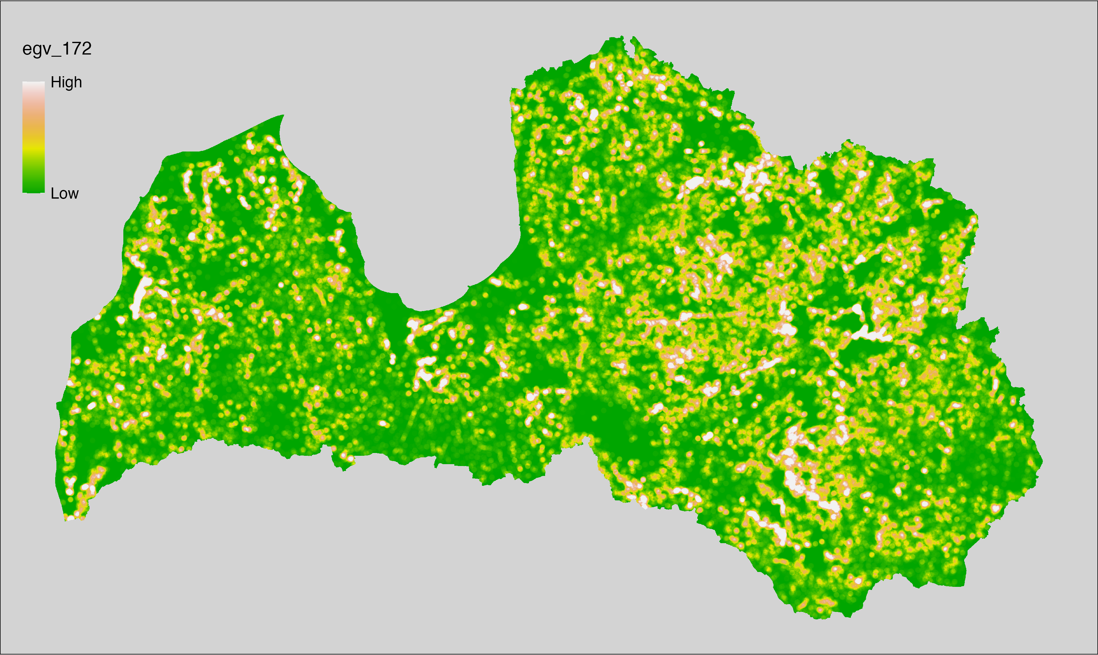
6.173 Edges_Water-Grassland_r3000
filename: Edges_Water-Grassland_r3000.tif
layername: egv_173
English name: Edge pixels of Water bordering with Grassland within the 3 km landscape
Latvian name: Ūdenstilpju malu ar zālājiem pikseļu skaits 3 km ainavā
Procedure: The total edge within a 3000 m radius around the analysis grid cell is
calculated as the area-weighted sum of the analysis cells inside the
buffer, using the workflow egvtools::radius_function(). During the calculation of the landscape metric,
inverse distance weighted (power = 2) gap filling on the output is applied
to ensure no missing values at the edges. Then the layer is rewritten to set
its name. Finally, the layer is standardised by subtracting the arithmetic
mean and dividing by the root mean squared error.
Code
# libs ----
if(!require(terra)) {install.packages("terra"); require(terra)}
if(!require(egvtools)) {remotes::install_github("aavotins/egvtools"); require(egvtools)}
# Templates -----
template100=rast("./Templates/TemplateRasters/LV100m_10km.tif")
# radii ----
radius_function(
kvadrati_path = "./Templates/TemplateGrids/tiles/",
radii_path = "./Templates/TemplateGridPoints/tiles/",
tikls100_path = "./Templates/TemplateGrids/tikls100_sauzeme.parquet",
template_path = "./Templates/TemplateRasters/LV100m_10km.tif",
input_layers = c("./RasterGrids_100m/2024/RAW/Edges_Water-Grassland_cell.tif"),
layer_prefixes = c("Edges_Water-Grassland"),
output_dir = "./RasterGrids_100m/2024/RAW/",
n_workers = 12,
radii = c("r3000"),
radius_mode = "sparse",
extract_fun = "sum",
fill_missing = TRUE,
IDW_weight = 2,
future_max_size = 20 * 1024^3)
# Edges_Water-Grassland_r3000.tif egv_173 ----
slanis=rast("./RasterGrids_100m/2024/RAW/Edges_Water-Grassland_r3000.tif")
names(slanis)="egv_173"
slanis2=project(slanis,template100)
writeRaster(slanis2,
"./RasterGrids_100m/2024/RAW/Edges_Water-Grassland_r3000.tif",
overwrite=TRUE)
# standardisation ----
if(!require(terra)) {install.packages("terra"); require(terra)}
if(!require(tidyverse)) {install.packages("tidyverse"); require(tidyverse)}
nosaukums="Edges_Water-Grassland_r3000.tif"
ielasisanas_cels=paste0("./RasterGrids_100m/2024/RAW/",nosaukums)
saglabasanas_cels=paste0("./RasterGrids_100m/2024/Scaled/",nosaukums)
slanis=rast(ielasisanas_cels)
videjais=global(slanis,fun="mean",na.rm=TRUE)
centrets=slanis-videjais[,1]
standartnovirze=terra::global(centrets,fun="rms",na.rm=TRUE)
merogots=centrets/standartnovirze[,1]
writeRaster(merogots,
filename=saglabasanas_cels,
overwrite=TRUE)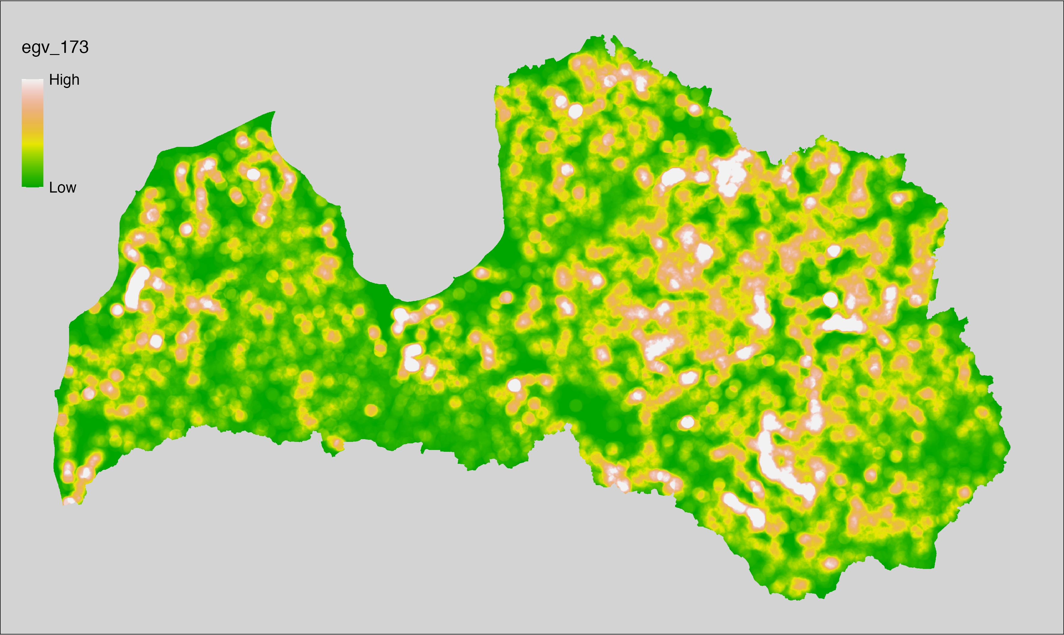
6.174 Edges_Water-Grassland_r10000
filename: Edges_Water-Grassland_r10000.tif
layername: egv_174
English name: Edge pixels of Water bordering with Grassland within the 10 km landscape
Latvian name: Ūdenstilpju malu ar zālājiem pikseļu skaits 10 km ainavā
Procedure: The total edge within a 10000 m radius around the analysis grid cell is
calculated as the area-weighted sum of the analysis cells inside the
buffer, using the workflow egvtools::radius_function(). During the calculation of the landscape metric,
inverse distance weighted (power = 2) gap filling on the output is applied
to ensure no missing values at the edges. Then the layer is rewritten to set
its name. Finally, the layer is standardised by subtracting the arithmetic
mean and dividing by the root mean squared error.
Code
# libs ----
if(!require(terra)) {install.packages("terra"); require(terra)}
if(!require(egvtools)) {remotes::install_github("aavotins/egvtools"); require(egvtools)}
# Templates -----
template100=rast("./Templates/TemplateRasters/LV100m_10km.tif")
# radii ----
radius_function(
kvadrati_path = "./Templates/TemplateGrids/tiles/",
radii_path = "./Templates/TemplateGridPoints/tiles/",
tikls100_path = "./Templates/TemplateGrids/tikls100_sauzeme.parquet",
template_path = "./Templates/TemplateRasters/LV100m_10km.tif",
input_layers = c("./RasterGrids_100m/2024/RAW/Edges_Water-Grassland_cell.tif"),
layer_prefixes = c("Edges_Water-Grassland"),
output_dir = "./RasterGrids_100m/2024/RAW/",
n_workers = 12,
radii = c("r3000"),
radius_mode = "sparse",
extract_fun = "sum",
fill_missing = TRUE,
IDW_weight = 2,
future_max_size = 20 * 1024^3)
# Edges_Water-Grassland_r10000.tif egv_174 ----
slanis=rast("./RasterGrids_100m/2024/RAW/Edges_Water-Grassland_r10000.tif")
names(slanis)="egv_174"
slanis2=project(slanis,template100)
writeRaster(slanis2,
"./RasterGrids_100m/2024/RAW/Edges_Water-Grassland_r10000.tif",
overwrite=TRUE)
# standardisation ----
if(!require(terra)) {install.packages("terra"); require(terra)}
if(!require(tidyverse)) {install.packages("tidyverse"); require(tidyverse)}
nosaukums="Edges_Water-Grassland_r10000.tif"
ielasisanas_cels=paste0("./RasterGrids_100m/2024/RAW/",nosaukums)
saglabasanas_cels=paste0("./RasterGrids_100m/2024/Scaled/",nosaukums)
slanis=rast(ielasisanas_cels)
videjais=global(slanis,fun="mean",na.rm=TRUE)
centrets=slanis-videjais[,1]
standartnovirze=terra::global(centrets,fun="rms",na.rm=TRUE)
merogots=centrets/standartnovirze[,1]
writeRaster(merogots,
filename=saglabasanas_cels,
overwrite=TRUE)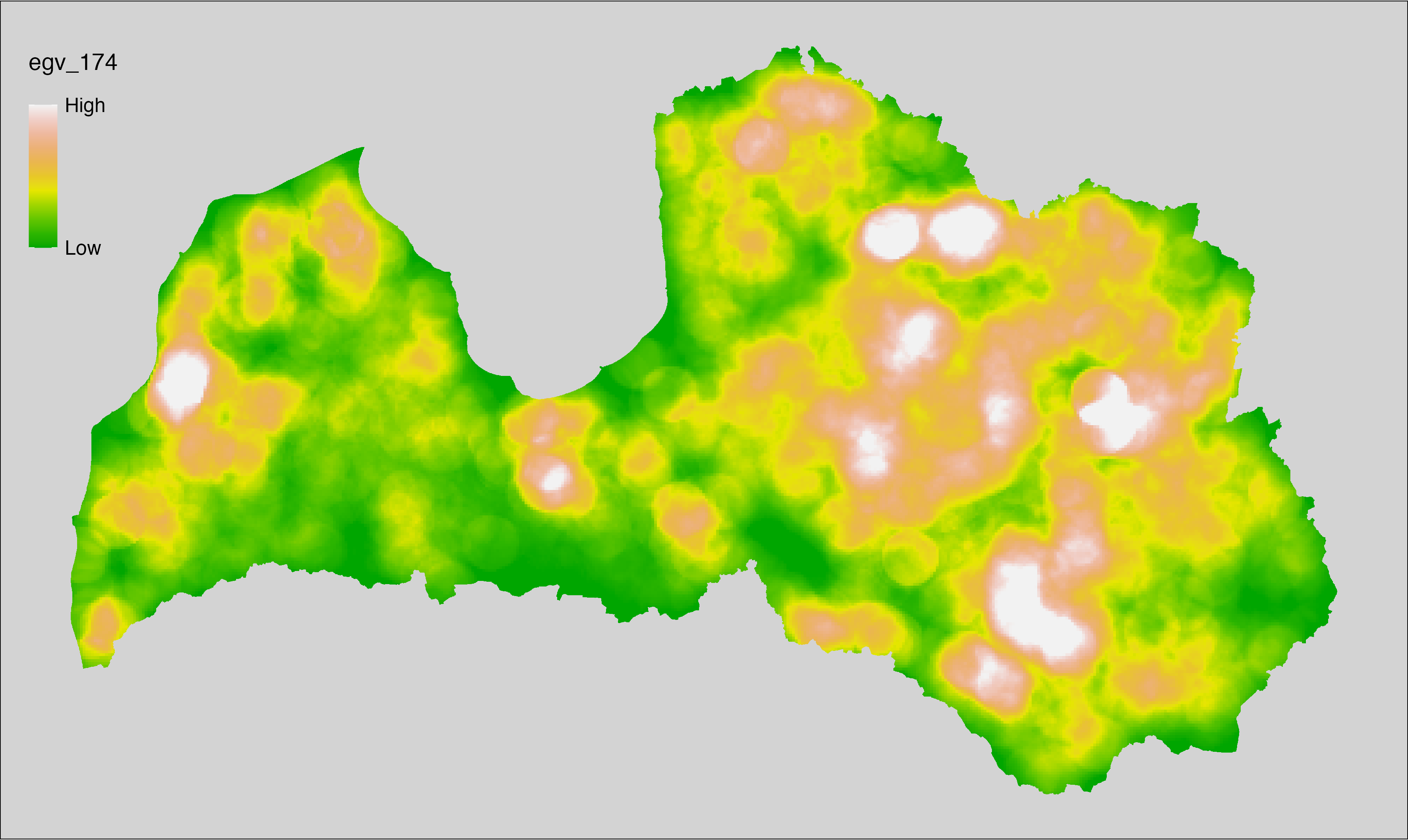
6.175 Edges_ReedSedgeRushBeds-Water_cell
filename: Edges_ReedSedgeRushBeds-Water_cell.tif
layername: egv_175
English name: Edge pixels of Reed-, Sedge-, Rush- Beds bordering with Water within the analysis cell (1 ha)
Latvian name: Niedrāju, grīslāju, meldrāju malu ar ūdeni pikseļu skaits analīzes šūnā (1 ha)
Procedure: First, values equal to 720 from the Landscape
classification are coded as 1, and all other values as NA. Then values
equal to 200 from the Landscape classification are coded as 0, and
all other values as NA. Then, the first layer (1 = presence) is covered over the
second layer (presence = 0) and written to file (matching the input). Next,
with the workflow egvtools::landscape_function() total edge between the two
classes is calculated. During the calculation of the landscape metric, inverse distance
weighted (power = 2) gap filling on the output is applied to ensure no
missing values at the edges. Finally, the layer is standardised by
subtracting the arithmetic mean and dividing by the root mean squared error.
Code
# libs ----
if(!require(terra)) {install.packages("terra"); require(terra)}
if(!require(egvtools)) {remotes::install_github("aavotins/egvtools"); require(egvtools)}
if(!require(sf)) {install.packages("sf"); require(sf)}
if(!require(sfarrow)) {install.packages("sfarrow"); require(sfarrow)}
if(!require(raster)) {install.packages("raster"); require(raster)}
if(!require(fasterize)) {install.packages("fasterize"); require(fasterize)}
if(!require(tidyverse)) {install.packages("tidyverse"); require(tidyverse)}
# Templates -----
template10=rast("./Templates/TemplateRasters/LV10m_10km.tif")
nulls10=rast("./Templates/TemplateRasters/nulls_LV10m_10km.tif")
# simple landscape ----
simple_landscape=rast("./RasterGrids_10m/2024/Ainava_vienk_mask.tif")
# Edges_ReedSedgeRushBeds-Water_input.tif ----
water=ifel(simple_landscape==200,0,NA)
plot(water)
reedsedgerush=ifel(simple_landscape==720,1,NA)
plot(reedsedgerush)
reedsedgerush_water=cover(reedsedgerush,water)
plot(reedsedgerush_water)
edge_reedsedgerush_water=project(reedsedgerush_water,template10,
filename="./RasterGrids_10m/2024/Edges_ReedSedgeRushBeds-Water_input.tif",
overwrite=TRUE)
rm(edge_reedsedgerush_water)
rm(reedsedgerush_water)
# Edges_ReedSedgeRushBeds-Water_cell.tif egv_175 ----
landscape_function(
landscape = "./RasterGrids_10m/2024/Edges_ReedSedgeRushBeds-Water_input.tif",
zones = "./Templates/TemplateGrids/tikls100_sauzeme.parquet",
id_field = "id",
tile_field = "tks50km",
template = "./Templates/TemplateRasters/LV100m_10km.tif",
out_dir = "./RasterGrids_100m/2024/RAW",
out_filename = "Edges_ReedSedgeRushBeds-Water_cell.tif",
out_layername = "egv_175",
what = "lsm_l_te",
lm_args = list(count_boundary = FALSE),
rasterize_engine = "fasterize",
n_workers = 12,
future_max_size = 20 * 1024^3,
fill_gaps = TRUE,
plot_gaps = FALSE,
plot_result = FALSE
)
# standardisation ----
if(!require(terra)) {install.packages("terra"); require(terra)}
if(!require(tidyverse)) {install.packages("tidyverse"); require(tidyverse)}
nosaukums="Edges_ReedSedgeRushBeds-Water_cell.tif"
ielasisanas_cels=paste0("./RasterGrids_100m/2024/RAW/",nosaukums)
saglabasanas_cels=paste0("./RasterGrids_100m/2024/Scaled/",nosaukums)
slanis=rast(ielasisanas_cels)
videjais=global(slanis,fun="mean",na.rm=TRUE)
centrets=slanis-videjais[,1]
standartnovirze=terra::global(centrets,fun="rms",na.rm=TRUE)
merogots=centrets/standartnovirze[,1]
writeRaster(merogots,
filename=saglabasanas_cels,
overwrite=TRUE)
6.176 Edges_ReedSedgeRushBeds-Water_r500
filename: Edges_ReedSedgeRushBeds-Water_r500.tif
layername: egv_176
English name: Edge pixels of Reed-, Sedge-, Rush- Beds bordering with Water within the 0.5 km landscape
Latvian name: Niedrāju, grīslāju, meldrāju malu ar ūdeni pikseļu skaits 0,5 km ainavā
Procedure: The total edge within a 500 m radius around the analysis grid cell is
calculated as the area-weighted sum of the analysis cells inside the
buffer, using the workflow egvtools::radius_function(). During the calculation of the landscape metric,
inverse distance weighted (power = 2) gap filling on the output is applied
to ensure no missing values at the edges. Then the layer is rewritten to set
its name. Finally, the layer is standardised by subtracting the arithmetic
mean and dividing by the root mean squared error.
Code
# libs ----
if(!require(terra)) {install.packages("terra"); require(terra)}
if(!require(egvtools)) {remotes::install_github("aavotins/egvtools"); require(egvtools)}
# Templates -----
template100=rast("./Templates/TemplateRasters/LV100m_10km.tif")
# radii ----
radius_function(
kvadrati_path = "./Templates/TemplateGrids/tiles/",
radii_path = "./Templates/TemplateGridPoints/tiles/",
tikls100_path = "./Templates/TemplateGrids/tikls100_sauzeme.parquet",
template_path = "./Templates/TemplateRasters/LV100m_10km.tif",
input_layers = c("./RasterGrids_100m/2024/RAW/Edges_ReedSedgeRushBeds-Water_cell.tif"),
layer_prefixes = c("Edges_ReedSedgeRushBeds-Water"),
output_dir = "./RasterGrids_100m/2024/RAW/",
n_workers = 12,
radii = c("r500"),
radius_mode = "sparse",
extract_fun = "sum",
fill_missing = TRUE,
IDW_weight = 2,
future_max_size = 20 * 1024^3)
# Edges_ReedSedgeRushBeds-Water_r500.tif egv_176 ----
slanis=rast("./RasterGrids_100m/2024/RAW/Edges_ReedSedgeRushBeds-Water_r500.tif")
names(slanis)="egv_176"
slanis2=project(slanis,template100)
writeRaster(slanis2,
"./RasterGrids_100m/2024/RAW/Edges_ReedSedgeRushBeds-Water_r500.tif",
overwrite=TRUE)
# standardisation ----
if(!require(terra)) {install.packages("terra"); require(terra)}
if(!require(tidyverse)) {install.packages("tidyverse"); require(tidyverse)}
nosaukums="Edges_ReedSedgeRushBeds-Water_r500.tif"
ielasisanas_cels=paste0("./RasterGrids_100m/2024/RAW/",nosaukums)
saglabasanas_cels=paste0("./RasterGrids_100m/2024/Scaled/",nosaukums)
slanis=rast(ielasisanas_cels)
videjais=global(slanis,fun="mean",na.rm=TRUE)
centrets=slanis-videjais[,1]
standartnovirze=terra::global(centrets,fun="rms",na.rm=TRUE)
merogots=centrets/standartnovirze[,1]
writeRaster(merogots,
filename=saglabasanas_cels,
overwrite=TRUE)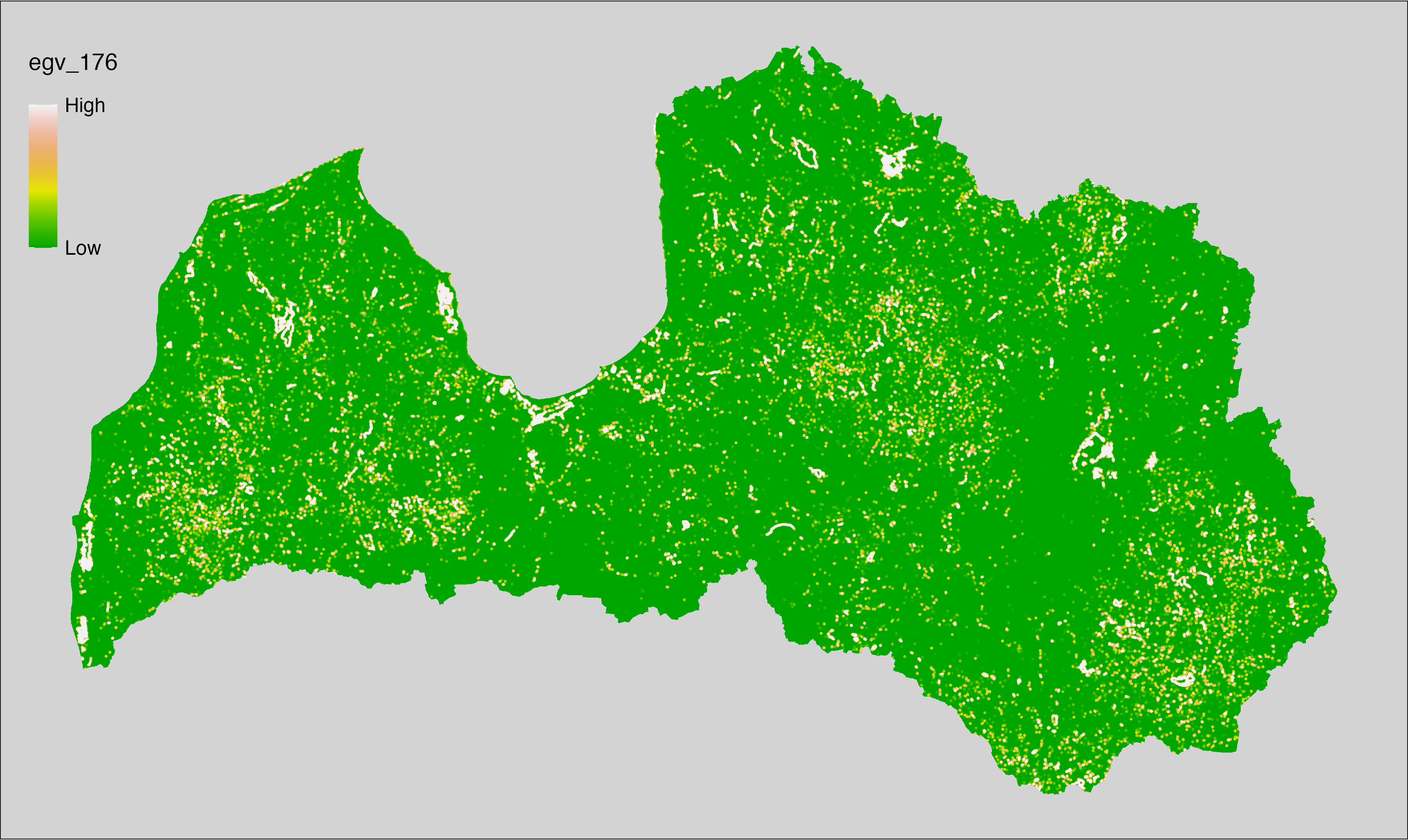
6.177 Edges_ReedSedgeRushBeds-Water_r1250
filename: Edges_ReedSedgeRushBeds-Water_r1250.tif
layername: egv_177
English name: Edge pixels of Reed-, Sedge-, Rush- Beds bordering with Water within the 1.25 km landscape
Latvian name: Niedrāju, grīslāju, meldrāju malu ar ūdeni pikseļu skaits 1,25 km ainavā
Procedure: The total edge within a 1250 m radius around the analysis grid cell is
calculated as the area-weighted sum of the analysis cells inside the
buffer, using the workflow egvtools::radius_function(). During the calculation of the landscape metric,
inverse distance weighted (power = 2) gap filling on the output is applied
to ensure no missing values at the edges. Then the layer is rewritten to set
its name. Finally, the layer is standardised by subtracting the arithmetic
mean and dividing by the root mean squared error.
Code
# libs ----
if(!require(terra)) {install.packages("terra"); require(terra)}
if(!require(egvtools)) {remotes::install_github("aavotins/egvtools"); require(egvtools)}
# Templates -----
template100=rast("./Templates/TemplateRasters/LV100m_10km.tif")
# radii ----
radius_function(
kvadrati_path = "./Templates/TemplateGrids/tiles/",
radii_path = "./Templates/TemplateGridPoints/tiles/",
tikls100_path = "./Templates/TemplateGrids/tikls100_sauzeme.parquet",
template_path = "./Templates/TemplateRasters/LV100m_10km.tif",
input_layers = c("./RasterGrids_100m/2024/RAW/Edges_ReedSedgeRushBeds-Water_cell.tif"),
layer_prefixes = c("Edges_ReedSedgeRushBeds-Water"),
output_dir = "./RasterGrids_100m/2024/RAW/",
n_workers = 12,
radii = c("r1250"),
radius_mode = "sparse",
extract_fun = "sum",
fill_missing = TRUE,
IDW_weight = 2,
future_max_size = 20 * 1024^3)
# Edges_ReedSedgeRushBeds-Water_r1250.tif egv_177 ----
slanis=rast("./RasterGrids_100m/2024/RAW/Edges_ReedSedgeRushBeds-Water_r1250.tif")
names(slanis)="egv_177"
slanis2=project(slanis,template100)
writeRaster(slanis2,
"./RasterGrids_100m/2024/RAW/Edges_ReedSedgeRushBeds-Water_r1250.tif",
overwrite=TRUE)
# standardisation ----
if(!require(terra)) {install.packages("terra"); require(terra)}
if(!require(tidyverse)) {install.packages("tidyverse"); require(tidyverse)}
nosaukums="Edges_ReedSedgeRushBeds-Water_r1250.tif"
ielasisanas_cels=paste0("./RasterGrids_100m/2024/RAW/",nosaukums)
saglabasanas_cels=paste0("./RasterGrids_100m/2024/Scaled/",nosaukums)
slanis=rast(ielasisanas_cels)
videjais=global(slanis,fun="mean",na.rm=TRUE)
centrets=slanis-videjais[,1]
standartnovirze=terra::global(centrets,fun="rms",na.rm=TRUE)
merogots=centrets/standartnovirze[,1]
writeRaster(merogots,
filename=saglabasanas_cels,
overwrite=TRUE)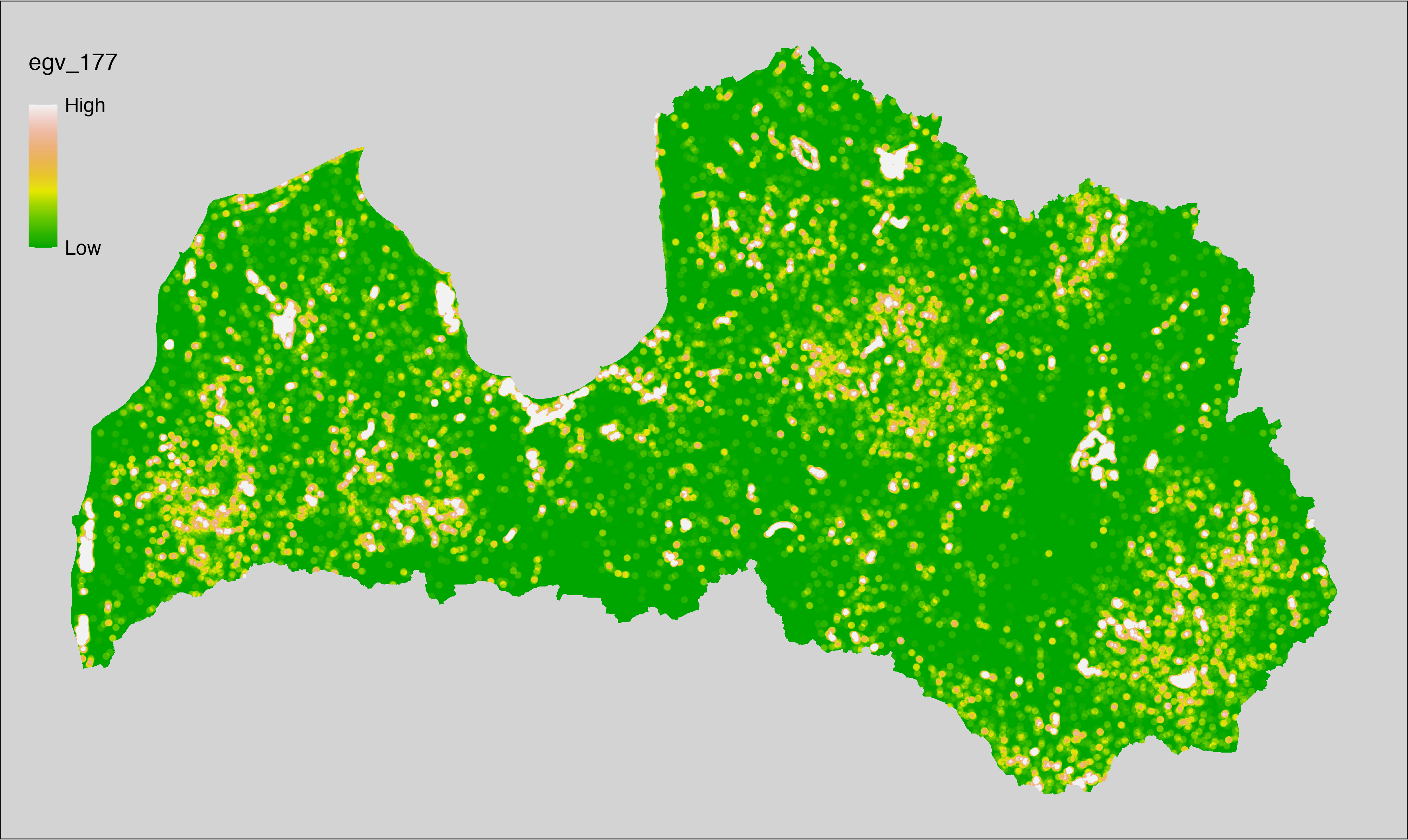
6.178 Edges_ReedSedgeRushBeds-Water_r3000
filename: Edges_ReedSedgeRushBeds-Water_r3000.tif
layername: egv_178
English name: Edge pixels of Reed-, Sedge-, Rush- Beds bordering with Water within the 3 km landscape
Latvian name: Niedrāju, grīslāju, meldrāju malu ar ūdeni pikseļu skaits 3 km ainavā
Procedure: The total edge within a 3000 m radius around the analysis grid cell is
calculated as the area-weighted sum of the analysis cells inside the
buffer, using the workflow egvtools::radius_function(). During the calculation of the landscape metric,
inverse distance weighted (power = 2) gap filling on the output is applied
to ensure no missing values at the edges. Then the layer is rewritten to set
its name. Finally, the layer is standardised by subtracting the arithmetic
mean and dividing by the root mean squared error.
Code
# libs ----
if(!require(terra)) {install.packages("terra"); require(terra)}
if(!require(egvtools)) {remotes::install_github("aavotins/egvtools"); require(egvtools)}
# Templates -----
template100=rast("./Templates/TemplateRasters/LV100m_10km.tif")
# radii ----
radius_function(
kvadrati_path = "./Templates/TemplateGrids/tiles/",
radii_path = "./Templates/TemplateGridPoints/tiles/",
tikls100_path = "./Templates/TemplateGrids/tikls100_sauzeme.parquet",
template_path = "./Templates/TemplateRasters/LV100m_10km.tif",
input_layers = c("./RasterGrids_100m/2024/RAW/Edges_ReedSedgeRushBeds-Water_cell.tif"),
layer_prefixes = c("Edges_ReedSedgeRushBeds-Water"),
output_dir = "./RasterGrids_100m/2024/RAW/",
n_workers = 12,
radii = c("r3000"),
radius_mode = "sparse",
extract_fun = "sum",
fill_missing = TRUE,
IDW_weight = 2,
future_max_size = 20 * 1024^3)
# Edges_ReedSedgeRushBeds-Water_r3000.tif egv_178 ----
slanis=rast("./RasterGrids_100m/2024/RAW/Edges_ReedSedgeRushBeds-Water_r3000.tif")
names(slanis)="egv_178"
slanis2=project(slanis,template100)
writeRaster(slanis2,
"./RasterGrids_100m/2024/RAW/Edges_ReedSedgeRushBeds-Water_r3000.tif",
overwrite=TRUE)
# standardisation ----
if(!require(terra)) {install.packages("terra"); require(terra)}
if(!require(tidyverse)) {install.packages("tidyverse"); require(tidyverse)}
nosaukums="Edges_ReedSedgeRushBeds-Water_r3000.tif"
ielasisanas_cels=paste0("./RasterGrids_100m/2024/RAW/",nosaukums)
saglabasanas_cels=paste0("./RasterGrids_100m/2024/Scaled/",nosaukums)
slanis=rast(ielasisanas_cels)
videjais=global(slanis,fun="mean",na.rm=TRUE)
centrets=slanis-videjais[,1]
standartnovirze=terra::global(centrets,fun="rms",na.rm=TRUE)
merogots=centrets/standartnovirze[,1]
writeRaster(merogots,
filename=saglabasanas_cels,
overwrite=TRUE)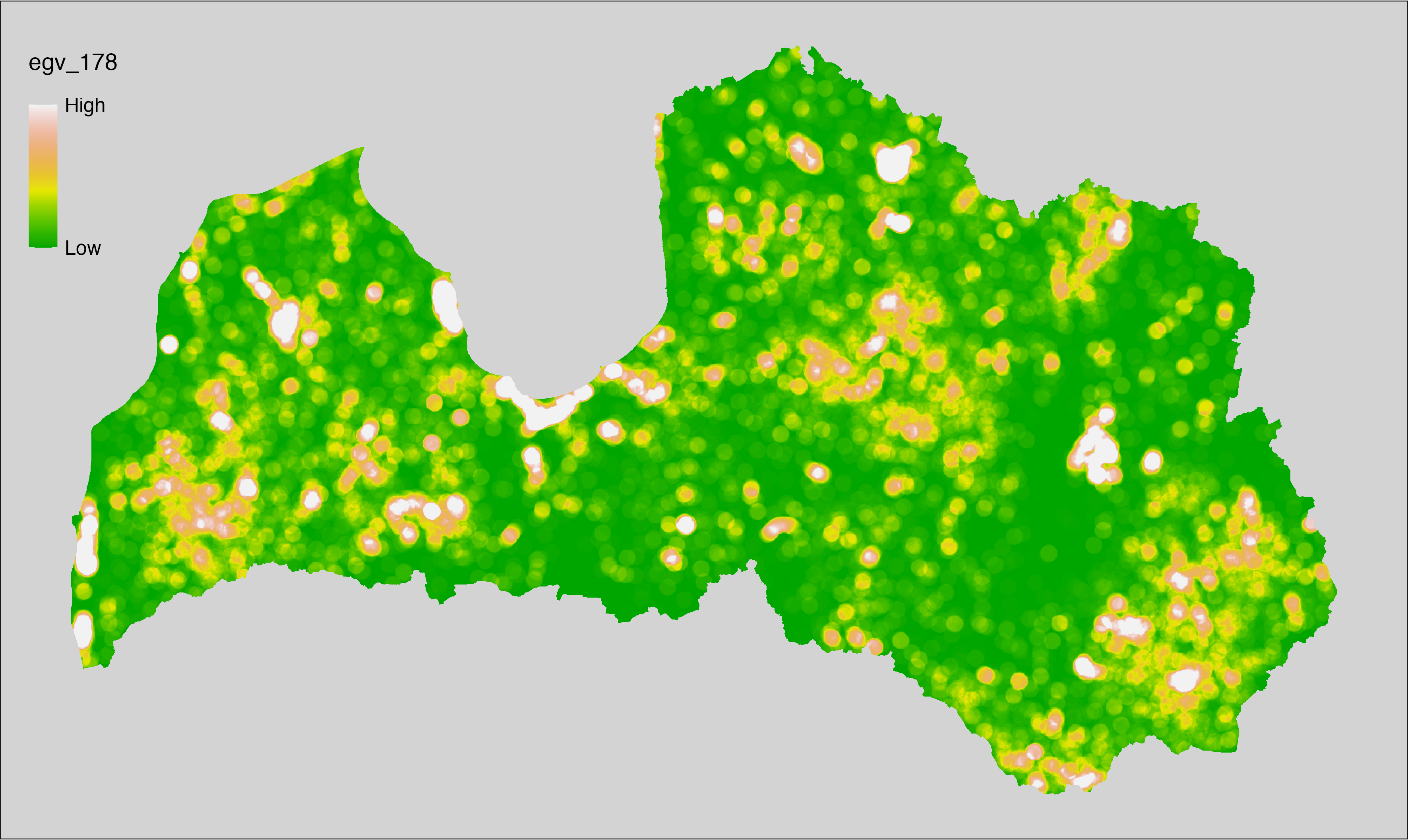
6.179 Edges_ReedSedgeRushBeds-Water_r10000
filename: Edges_ReedSedgeRushBeds-Water_r10000.tif
layername: egv_179
English name: Edge pixels of Reed-, Sedge-, Rush- Beds bordering with Water within the 10 km landscape
Latvian name: Niedrāju, grīslāju, meldrāju malu ar ūdeni pikseļu skaits 10 km ainavā
Procedure: The total edge within a 10000 m radius around the analysis grid cell is
calculated as the area-weighted sum of the analysis cells inside the
buffer, using the workflow egvtools::radius_function(). During the calculation of the landscape metric,
inverse distance weighted (power = 2) gap filling on the output is applied
to ensure no missing values at the edges. Then the layer is rewritten to set
its name. Finally, the layer is standardised by subtracting the arithmetic
mean and dividing by the root mean squared error.
Code
# libs ----
if(!require(terra)) {install.packages("terra"); require(terra)}
if(!require(egvtools)) {remotes::install_github("aavotins/egvtools"); require(egvtools)}
# Templates -----
template100=rast("./Templates/TemplateRasters/LV100m_10km.tif")
# radii ----
radius_function(
kvadrati_path = "./Templates/TemplateGrids/tiles/",
radii_path = "./Templates/TemplateGridPoints/tiles/",
tikls100_path = "./Templates/TemplateGrids/tikls100_sauzeme.parquet",
template_path = "./Templates/TemplateRasters/LV100m_10km.tif",
input_layers = c("./RasterGrids_100m/2024/RAW/Edges_ReedSedgeRushBeds-Water_cell.tif"),
layer_prefixes = c("Edges_ReedSedgeRushBeds-Water"),
output_dir = "./RasterGrids_100m/2024/RAW/",
n_workers = 12,
radii = c("r10000"),
radius_mode = "sparse",
extract_fun = "sum",
fill_missing = TRUE,
IDW_weight = 2,
future_max_size = 20 * 1024^3)
# Edges_ReedSedgeRushBeds-Water_r10000.tif egv_179 ----
slanis=rast("./RasterGrids_100m/2024/RAW/Edges_ReedSedgeRushBeds-Water_r10000.tif")
names(slanis)="egv_179"
slanis2=project(slanis,template100)
writeRaster(slanis2,
"./RasterGrids_100m/2024/RAW/Edges_ReedSedgeRushBeds-Water_r10000.tif",
overwrite=TRUE)
# standardisation ----
if(!require(terra)) {install.packages("terra"); require(terra)}
if(!require(tidyverse)) {install.packages("tidyverse"); require(tidyverse)}
nosaukums="Edges_ReedSedgeRushBeds-Water_r10000.tif"
ielasisanas_cels=paste0("./RasterGrids_100m/2024/RAW/",nosaukums)
saglabasanas_cels=paste0("./RasterGrids_100m/2024/Scaled/",nosaukums)
slanis=rast(ielasisanas_cels)
videjais=global(slanis,fun="mean",na.rm=TRUE)
centrets=slanis-videjais[,1]
standartnovirze=terra::global(centrets,fun="rms",na.rm=TRUE)
merogots=centrets/standartnovirze[,1]
writeRaster(merogots,
filename=saglabasanas_cels,
overwrite=TRUE)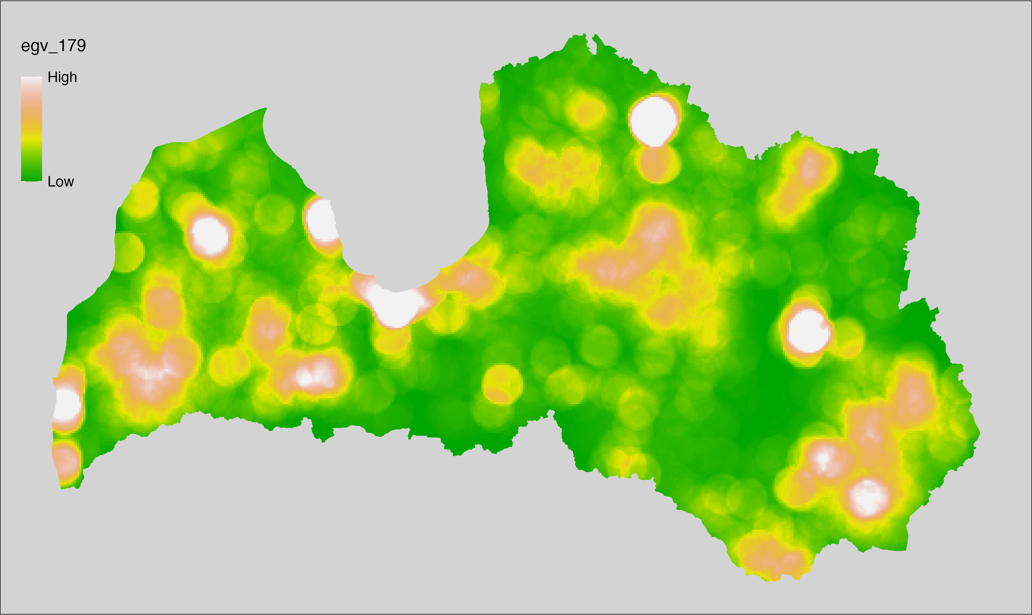
6.180 FarmlandCrops_CropsAll_cell
filename: FarmlandCrops_CropsAll_cell.tif
layername: egv_180
English name: Fractional cover of Crops (all types) within the analysis cell (1 ha)
Latvian name: Aramzemju (dažādu lauksaimniecības kultūraugu) platības īpatsvars analīzes šūnā (1 ha)
Procedure: First, agricultural parcels with any type of crops are selected
from the Rural Support Service’s information on declared fields. These
geometries are then rasterised to input resolution, ensuring value 1 at the
polygon locations and value 0 elsewhere. Rasterisation is performed with the workflow
egvtools::polygon2input(). Once rasterised, the layer is aggregated to EGV
resolution using the workflow egvtools::input2egv(), which calculates the arithmetic mean and thus
results in a cover fraction. During aggregation, inverse distance weighted
(power = 2) gap filling on the output is applied to ensure no missing
values at the edges. Finally, the layer is standardised by subtracting
the arithmetic mean and dividing by the root mean squared error.
Code
# libs ----
if(!require(egvtools)) {remotes::install_github("aavotins/egvtools"); require(egvtools)}
if(!require(terra)) {install.packages("terra"); require(terra)}
if(!require(sf)) {install.packages("sf"); require(sf)}
if(!require(tidyverse)) {install.packages("tidyverse"); require(tidyverse)}
if(!require(sfarrow)) {install.packages("sfarrow"); require(sfarrow)}
if(!require(readxl)) {install.packages("readxl"); require(readxl)}
if(!require(raster)) {install.packages("raster"); require(raster)}
if(!require(fasterize)) {install.packages("fasterize"); require(fasterize)}
# templates ----
template100=rast("./Templates/TemplateRasters/LV100m_10km.tif")
template10=rast("./Templates/TemplateRasters/LV10m_10km.tif")
rastrs10=raster(template10)
nulls10=rast("./Templates/TemplateRasters/nulls_LV10m_10km.tif")
nulls100=rast("./Templates/TemplateRasters/nulls_LV100m_10km.tif")
# codes ----
kodi=read_excel("./Geodata/2024/LAD/KulturuKodi_2024.xlsx")
kodi$kods=as.character(kodi$kods)
# LAD ----
lad=sfarrow::st_read_parquet("./Geodata/2024/LAD/Lauki_2024.parquet")
lad$yes=1
lad=lad %>%
left_join(kodi,by=c("PRODUCT_CODE"="kods"))
# simple landscape ----
simple_landscape=rast("RasterGrids_10m/2024/Ainava_vienk_mask.tif")
# FarmlandCrops_CropsAll_cell.tif egv_180 ----
aramzemes=lad %>%
filter(str_detect(SDM_grupa_sakums,"aramz"))
p2i_rez=egvtools::polygon2input(vector_data = aramzemes,
template_path = "./Templates/TemplateRasters/LV10m_10km.tif",
out_path = "./RasterGrids_10m/2024/",
file_name = "FarmlandCrops_CropsAll_input.tif",
value_field = "yes",
prepare=FALSE,
background_raster = "./Templates/TemplateRasters/nulls_LV10m_10km.tif",
plot_result = TRUE)
p2i_rez
i2e_rez=egvtools::input2egv(input=paste0("./RasterGrids_10m/2024/",
"FarmlandCrops_CropsAll_input.tif"),
egv_template= "./Templates/TemplateRasters/LV100m_10km.tif",
summary_function = "average",
missing_job = "FillOutput",
outlocation = "./RasterGrids_100m/2024/RAW/",
outfilename = "FarmlandCrops_CropsAll_cell.tif",
layername = "egv_180",
idw_weight = 2,
plot_gaps = FALSE,plot_final = TRUE)
i2e_rez
rm(p2i_rez)
rm(i2e_rez)
rm(aramzemes)
unlink("./RasterGrids_10m/2024/FarmlandCrops_CropsAll_input.tif")
# standardisation ----
if(!require(terra)) {install.packages("terra"); require(terra)}
if(!require(tidyverse)) {install.packages("tidyverse"); require(tidyverse)}
nosaukums="FarmlandCrops_CropsAll_cell.tif"
ielasisanas_cels=paste0("./RasterGrids_100m/2024/RAW/",nosaukums)
saglabasanas_cels=paste0("./RasterGrids_100m/2024/Scaled/",nosaukums)
slanis=rast(ielasisanas_cels)
videjais=global(slanis,fun="mean",na.rm=TRUE)
centrets=slanis-videjais[,1]
standartnovirze=terra::global(centrets,fun="rms",na.rm=TRUE)
merogots=centrets/standartnovirze[,1]
writeRaster(merogots,
filename=saglabasanas_cels,
overwrite=TRUE)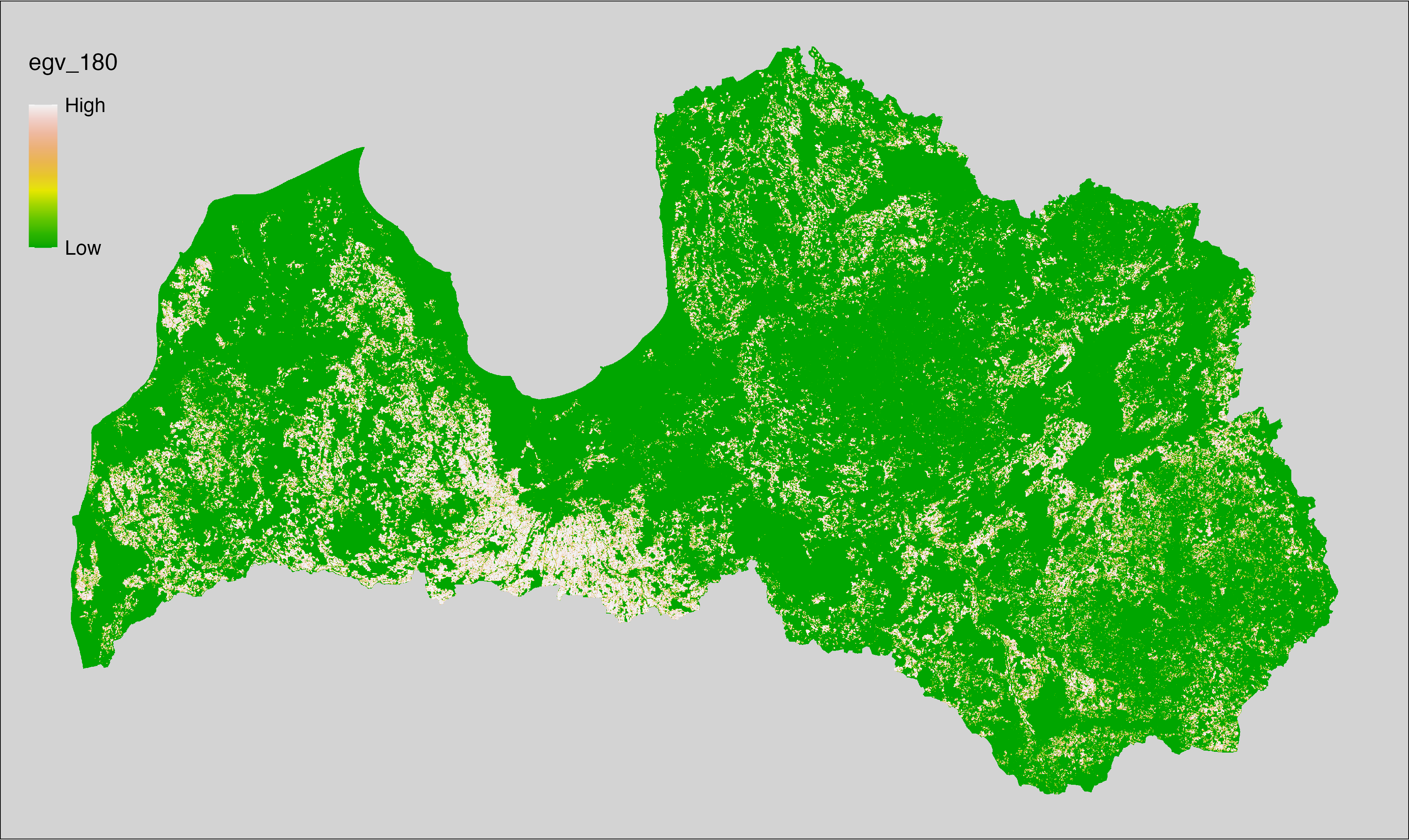
6.181 FarmlandCrops_CropsAll_r500
filename: FarmlandCrops_CropsAll_r500.tif
layername: egv_181
English name: Fractional cover of Crops (all types) within the 0.5 km landscape
Latvian name: Aramzemju (dažādu lauksaimniecības kultūraugu) platības īpatsvars 0,5 km ainavā
Procedure: The cover fraction within a radius of 500 m around the analysis grid cell is
calculated as the area-weighted sum of the analysis cells inside the
buffer, using the workflow egvtools::radius_function(). During the calculation of the landscape metric,
inverse distance weighted (power = 2) gap filling on the output is applied
to ensure no missing values at the edges. Then the layer is rewritten to set
its name. Finally, the layer is standardised by subtracting the arithmetic
mean and dividing by the root mean squared error.
Code
# libs ----
if(!require(terra)) {install.packages("terra"); require(terra)}
if(!require(egvtools)) {remotes::install_github("aavotins/egvtools"); require(egvtools)}
# Templates -----
template100=rast("./Templates/TemplateRasters/LV100m_10km.tif")
# radii ----
radius_function(
kvadrati_path = "./Templates/TemplateGrids/tiles/",
radii_path = "./Templates/TemplateGridPoints/tiles/",
tikls100_path = "./Templates/TemplateGrids/tikls100_sauzeme.parquet",
template_path = "./Templates/TemplateRasters/LV100m_10km.tif",
input_layers = c("./RasterGrids_100m/2024/RAW/FarmlandCrops_CropsAll_cell.tif"),
layer_prefixes = c("FarmlandCrops_CropsAll"),
output_dir = "./RasterGrids_100m/2024/RAW/",
n_workers = 6,
radii = c("r500"),
radius_mode = "sparse",
extract_fun = "mean",
fill_missing = TRUE,
IDW_weight = 2,
future_max_size = 40 * 1024^3)
# FarmlandCrops_CropsAll_r500.tif egv_181 ----
slanis=rast("./RasterGrids_100m/2024/RAW/FarmlandCrops_CropsAll_r500.tif")
names(slanis)="egv_181"
slanis2=project(slanis,template100)
writeRaster(slanis2,
"./RasterGrids_100m/2024/RAW/FarmlandCrops_CropsAll_r500.tif",
overwrite=TRUE)
# standardisation ----
if(!require(terra)) {install.packages("terra"); require(terra)}
if(!require(tidyverse)) {install.packages("tidyverse"); require(tidyverse)}
nosaukums="FarmlandCrops_CropsAll_r500.tif"
ielasisanas_cels=paste0("./RasterGrids_100m/2024/RAW/",nosaukums)
saglabasanas_cels=paste0("./RasterGrids_100m/2024/Scaled/",nosaukums)
slanis=rast(ielasisanas_cels)
videjais=global(slanis,fun="mean",na.rm=TRUE)
centrets=slanis-videjais[,1]
standartnovirze=terra::global(centrets,fun="rms",na.rm=TRUE)
merogots=centrets/standartnovirze[,1]
writeRaster(merogots,
filename=saglabasanas_cels,
overwrite=TRUE)
6.182 FarmlandCrops_CropsAll_r1250
filename: FarmlandCrops_CropsAll_r1250.tif
layername: egv_182
English name: Fractional cover of Crops (all types) within the 1.25 km landscape
Latvian name: Aramzemju (dažādu lauksaimniecības kultūraugu) platības īpatsvars 1,25 km ainavā
Procedure: The cover fraction within a radius of 1250 m around the analysis grid cell
is calculated as the area-weighted sum of the analysis cells inside
the buffer, using the workflow egvtools::radius_function(). During the calculation of the landscape
metric, inverse distance weighted (power = 2) gap filling on the output is
applied to ensure no missing values at the edges. Then the layer is
rewritten to set its name. Finally, the layer is standardised by
subtracting the arithmetic mean and dividing by the root mean squared error.
Code
# libs ----
if(!require(terra)) {install.packages("terra"); require(terra)}
if(!require(egvtools)) {remotes::install_github("aavotins/egvtools"); require(egvtools)}
# Templates -----
template100=rast("./Templates/TemplateRasters/LV100m_10km.tif")
# radii ----
radius_function(
kvadrati_path = "./Templates/TemplateGrids/tiles/",
radii_path = "./Templates/TemplateGridPoints/tiles/",
tikls100_path = "./Templates/TemplateGrids/tikls100_sauzeme.parquet",
template_path = "./Templates/TemplateRasters/LV100m_10km.tif",
input_layers = c("./RasterGrids_100m/2024/RAW/FarmlandCrops_CropsAll_cell.tif"),
layer_prefixes = c("FarmlandCrops_CropsAll"),
output_dir = "./RasterGrids_100m/2024/RAW/",
n_workers = 6,
radii = c("r1250"),
radius_mode = "sparse",
extract_fun = "mean",
fill_missing = TRUE,
IDW_weight = 2,
future_max_size = 40 * 1024^3)
# FarmlandCrops_CropsAll_r1250.tif egv_182 ----
slanis=rast("./RasterGrids_100m/2024/RAW/FarmlandCrops_CropsAll_r1250.tif")
names(slanis)="egv_182"
slanis2=project(slanis,template100)
writeRaster(slanis2,
"./RasterGrids_100m/2024/RAW/FarmlandCrops_CropsAll_r1250.tif",
overwrite=TRUE)
# standardisation ----
if(!require(terra)) {install.packages("terra"); require(terra)}
if(!require(tidyverse)) {install.packages("tidyverse"); require(tidyverse)}
nosaukums="FarmlandCrops_CropsAll_r1250.tif"
ielasisanas_cels=paste0("./RasterGrids_100m/2024/RAW/",nosaukums)
saglabasanas_cels=paste0("./RasterGrids_100m/2024/Scaled/",nosaukums)
slanis=rast(ielasisanas_cels)
videjais=global(slanis,fun="mean",na.rm=TRUE)
centrets=slanis-videjais[,1]
standartnovirze=terra::global(centrets,fun="rms",na.rm=TRUE)
merogots=centrets/standartnovirze[,1]
writeRaster(merogots,
filename=saglabasanas_cels,
overwrite=TRUE)
6.183 FarmlandCrops_CropsAll_r3000
filename: FarmlandCrops_CropsAll_r3000.tif
layername: egv_183
English name: Fractional cover of Crops (all types) within the 3 km landscape
Latvian name: Aramzemju (dažādu lauksaimniecības kultūraugu) platības īpatsvars 3 km ainavā
Procedure: The cover fraction within a radius of 3000 m around the analysis grid cell
is calculated as the area-weighted sum of the analysis cells inside
the buffer, using the workflow egvtools::radius_function(). During the calculation of the landscape
metric, inverse distance weighted (power = 2) gap filling on the output is
applied to ensure no missing values at the edges. Then the layer is
rewritten to set its name. Finally, the layer is standardised by
subtracting the arithmetic mean and dividing by the root mean squared error.
Code
# libs ----
if(!require(terra)) {install.packages("terra"); require(terra)}
if(!require(egvtools)) {remotes::install_github("aavotins/egvtools"); require(egvtools)}
# Templates -----
template100=rast("./Templates/TemplateRasters/LV100m_10km.tif")
# radii ----
radius_function(
kvadrati_path = "./Templates/TemplateGrids/tiles/",
radii_path = "./Templates/TemplateGridPoints/tiles/",
tikls100_path = "./Templates/TemplateGrids/tikls100_sauzeme.parquet",
template_path = "./Templates/TemplateRasters/LV100m_10km.tif",
input_layers = c("./RasterGrids_100m/2024/RAW/FarmlandCrops_CropsAll_cell.tif"),
layer_prefixes = c("FarmlandCrops_CropsAll"),
output_dir = "./RasterGrids_100m/2024/RAW/",
n_workers = 6,
radii = c("r3000"),
radius_mode = "sparse",
extract_fun = "mean",
fill_missing = TRUE,
IDW_weight = 2,
future_max_size = 40 * 1024^3)
# FarmlandCrops_CropsAll_r3000.tif egv_183 ----
slanis=rast("./RasterGrids_100m/2024/RAW/FarmlandCrops_CropsAll_r3000.tif")
names(slanis)="egv_183"
slanis2=project(slanis,template100)
writeRaster(slanis2,
"./RasterGrids_100m/2024/RAW/FarmlandCrops_CropsAll_r3000.tif",
overwrite=TRUE)
# standardisation ----
if(!require(terra)) {install.packages("terra"); require(terra)}
if(!require(tidyverse)) {install.packages("tidyverse"); require(tidyverse)}
nosaukums="FarmlandCrops_CropsAll_r3000.tif"
ielasisanas_cels=paste0("./RasterGrids_100m/2024/RAW/",nosaukums)
saglabasanas_cels=paste0("./RasterGrids_100m/2024/Scaled/",nosaukums)
slanis=rast(ielasisanas_cels)
videjais=global(slanis,fun="mean",na.rm=TRUE)
centrets=slanis-videjais[,1]
standartnovirze=terra::global(centrets,fun="rms",na.rm=TRUE)
merogots=centrets/standartnovirze[,1]
writeRaster(merogots,
filename=saglabasanas_cels,
overwrite=TRUE)
6.184 FarmlandCrops_CropsAll_r10000
filename: FarmlandCrops_CropsAll_r10000.tif
layername: egv_184
English name: Fractional cover of Crops (all types) within the 10 km landscape
Latvian name: Aramzemju (dažādu lauksaimniecības kultūraugu) platības īpatsvars 10 km ainavā
Procedure: The cover fraction within a radius of 10000 m around the analysis grid cell
is calculated as the area-weighted sum of the analysis cells inside
the buffer, using the workflow egvtools::radius_function(). During the calculation of the landscape
metric, inverse distance weighted (power = 2) gap filling on the output is
applied to ensure no missing values at the edges. Then the layer is
rewritten to set its name. Finally, the layer is standardised by
subtracting the arithmetic mean and dividing by the root mean squared error.
Code
# libs ----
if(!require(terra)) {install.packages("terra"); require(terra)}
if(!require(egvtools)) {remotes::install_github("aavotins/egvtools"); require(egvtools)}
# Templates -----
template100=rast("./Templates/TemplateRasters/LV100m_10km.tif")
# radii ----
radius_function(
kvadrati_path = "./Templates/TemplateGrids/tiles/",
radii_path = "./Templates/TemplateGridPoints/tiles/",
tikls100_path = "./Templates/TemplateGrids/tikls100_sauzeme.parquet",
template_path = "./Templates/TemplateRasters/LV100m_10km.tif",
input_layers = c("./RasterGrids_100m/2024/RAW/FarmlandCrops_CropsAll_cell.tif"),
layer_prefixes = c("FarmlandCrops_CropsAll"),
output_dir = "./RasterGrids_100m/2024/RAW/",
n_workers = 6,
radii = c("r10000"),
radius_mode = "sparse",
extract_fun = "mean",
fill_missing = TRUE,
IDW_weight = 2,
future_max_size = 40 * 1024^3)
# FarmlandCrops_CropsAll_r10000.tif egv_184 ----
slanis=rast("./RasterGrids_100m/2024/RAW/FarmlandCrops_CropsAll_r10000.tif")
names(slanis)="egv_184"
slanis2=project(slanis,template100)
writeRaster(slanis2,
"./RasterGrids_100m/2024/RAW/FarmlandCrops_CropsAll_r10000.tif",
overwrite=TRUE)
# standardisation ----
if(!require(terra)) {install.packages("terra"); require(terra)}
if(!require(tidyverse)) {install.packages("tidyverse"); require(tidyverse)}
nosaukums="FarmlandCrops_CropsAll_r10000.tif"
ielasisanas_cels=paste0("./RasterGrids_100m/2024/RAW/",nosaukums)
saglabasanas_cels=paste0("./RasterGrids_100m/2024/Scaled/",nosaukums)
slanis=rast(ielasisanas_cels)
videjais=global(slanis,fun="mean",na.rm=TRUE)
centrets=slanis-videjais[,1]
standartnovirze=terra::global(centrets,fun="rms",na.rm=TRUE)
merogots=centrets/standartnovirze[,1]
writeRaster(merogots,
filename=saglabasanas_cels,
overwrite=TRUE)
6.185 FarmlandCrops_CropsHoed_cell
filename: FarmlandCrops_CropsHoed_cell.tif
layername: egv_185
English name: Fractional cover of Hoed Crops within the analysis cell (1 ha)
Latvian name: Vagu un rušināmkultūru platības īpatsvars analīzes šūnā (1 ha)
Procedure: First, agricultural parcels declared as hoed crops are selected from the
Rural Support Service’s information on declared fields. These
geometries are then rasterised to input resolution, ensuring value 1 at the
polygon locations and value 0 elsewhere. Rasterisation is performed using the workflow
egvtools::polygon2input(). Once rasterised, the layer is aggregated to EGV
resolution using the workflow egvtools::input2egv(), which calculates the arithmetic mean and thus
results in a cover fraction. During aggregation, inverse distance weighted
(power = 2) gap filling on the output is applied to ensure no missing
values at the edges. Finally, the layer is standardised by subtracting
the arithmetic mean and dividing by the root mean squared error.
Code
# libs ----
if(!require(egvtools)) {remotes::install_github("aavotins/egvtools"); require(egvtools)}
if(!require(terra)) {install.packages("terra"); require(terra)}
if(!require(sf)) {install.packages("sf"); require(sf)}
if(!require(tidyverse)) {install.packages("tidyverse"); require(tidyverse)}
if(!require(sfarrow)) {install.packages("sfarrow"); require(sfarrow)}
if(!require(readxl)) {install.packages("readxl"); require(readxl)}
if(!require(raster)) {install.packages("raster"); require(raster)}
if(!require(fasterize)) {install.packages("fasterize"); require(fasterize)}
# templates ----
template100=rast("./Templates/TemplateRasters/LV100m_10km.tif")
template10=rast("./Templates/TemplateRasters/LV10m_10km.tif")
rastrs10=raster(template10)
nulls10=rast("./Templates/TemplateRasters/nulls_LV10m_10km.tif")
nulls100=rast("./Templates/TemplateRasters/nulls_LV100m_10km.tif")
# codes ----
kodi=read_excel("./Geodata/2024/LAD/KulturuKodi_2024.xlsx")
kodi$kods=as.character(kodi$kods)
# LAD ----
lad=sfarrow::st_read_parquet("./Geodata/2024/LAD/Lauki_2024.parquet")
lad$yes=1
lad=lad %>%
left_join(kodi,by=c("PRODUCT_CODE"="kods"))
# simple landscape ----
simple_landscape=rast("RasterGrids_10m/2024/Ainava_vienk_mask.tif")
# FarmlandCrops_CropsHoed_cell.tif egv_185 ----
dati=lad %>%
filter(str_detect(SDM_grupa_sakums,"ruši"))
table(dati$SDM_grupa_sakums,useNA="always")
p2i_rez=egvtools::polygon2input(vector_data = dati,
template_path = "./Templates/TemplateRasters/LV10m_10km.tif",
out_path = "./RasterGrids_10m/2024/",
file_name = "FarmlandCrops_CropsHoed_input.tif",
value_field = "yes",
prepare=FALSE,
background_raster = "./Templates/TemplateRasters/nulls_LV10m_10km.tif",
plot_result = TRUE)
p2i_rez
i2e_rez=egvtools::input2egv(input=paste0("./RasterGrids_10m/2024/",
"FarmlandCrops_CropsHoed_input.tif"),
egv_template= "./Templates/TemplateRasters/LV100m_10km.tif",
summary_function = "average",
missing_job = "FillOutput",
outlocation = "./RasterGrids_100m/2024/RAW/",
outfilename = "FarmlandCrops_CropsHoed_cell.tif",
layername = "egv_185",
idw_weight = 2,
plot_gaps = FALSE,plot_final = TRUE)
i2e_rez
rm(p2i_rez)
rm(i2e_rez)
rm(dati)
unlink("./RasterGrids_10m/2024/FarmlandCrops_CropsHoed_input.tif")
# standardisation ----
if(!require(terra)) {install.packages("terra"); require(terra)}
if(!require(tidyverse)) {install.packages("tidyverse"); require(tidyverse)}
nosaukums="FarmlandCrops_CropsHoed_cell.tif"
ielasisanas_cels=paste0("./RasterGrids_100m/2024/RAW/",nosaukums)
saglabasanas_cels=paste0("./RasterGrids_100m/2024/Scaled/",nosaukums)
slanis=rast(ielasisanas_cels)
videjais=global(slanis,fun="mean",na.rm=TRUE)
centrets=slanis-videjais[,1]
standartnovirze=terra::global(centrets,fun="rms",na.rm=TRUE)
merogots=centrets/standartnovirze[,1]
writeRaster(merogots,
filename=saglabasanas_cels,
overwrite=TRUE)
6.186 FarmlandCrops_CropsHoed_r500
filename: FarmlandCrops_CropsHoed_r500.tif
layername: egv_186
English name: Fractional cover of Hoed Crops within the 0.5 km landscape
Latvian name: Vagu un rušināmkultūru platības īpatsvars 0,5 km ainavā
Procedure: The cover fraction within a radius of 500 m around the analysis grid cell is
calculated as the area-weighted sum of the analysis cells inside the
buffer, using the workflow egvtools::radius_function(). During the calculation of the landscape metric,
inverse distance weighted (power = 2) gap filling on the output is applied
to ensure no missing values at the edges. Then the layer is rewritten to set
its name. Finally, the layer is standardised by subtracting the arithmetic
mean and dividing by the root mean squared error.
Code
# libs ----
if(!require(terra)) {install.packages("terra"); require(terra)}
if(!require(egvtools)) {remotes::install_github("aavotins/egvtools"); require(egvtools)}
# Templates -----
template100=rast("./Templates/TemplateRasters/LV100m_10km.tif")
# radii ----
radius_function(
kvadrati_path = "./Templates/TemplateGrids/tiles/",
radii_path = "./Templates/TemplateGridPoints/tiles/",
tikls100_path = "./Templates/TemplateGrids/tikls100_sauzeme.parquet",
template_path = "./Templates/TemplateRasters/LV100m_10km.tif",
input_layers = c("./RasterGrids_100m/2024/RAW/FarmlandCrops_CropsHoed_cell.tif"),
layer_prefixes = c("FarmlandCrops_CropsHoed"),
output_dir = "./RasterGrids_100m/2024/RAW/",
n_workers = 6,
radii = c("r500"),
radius_mode = "sparse",
extract_fun = "mean",
fill_missing = TRUE,
IDW_weight = 2,
future_max_size = 40 * 1024^3)
# FarmlandCrops_CropsHoed_r500.tif egv_186 ----
slanis=rast("./RasterGrids_100m/2024/RAW/FarmlandCrops_CropsHoed_r500.tif")
names(slanis)="egv_186"
slanis2=project(slanis,template100)
writeRaster(slanis2,
"./RasterGrids_100m/2024/RAW/FarmlandCrops_CropsHoed_r500.tif",
overwrite=TRUE)
# standardisation ----
if(!require(terra)) {install.packages("terra"); require(terra)}
if(!require(tidyverse)) {install.packages("tidyverse"); require(tidyverse)}
nosaukums="FarmlandCrops_CropsHoed_r500.tif"
ielasisanas_cels=paste0("./RasterGrids_100m/2024/RAW/",nosaukums)
saglabasanas_cels=paste0("./RasterGrids_100m/2024/Scaled/",nosaukums)
slanis=rast(ielasisanas_cels)
videjais=global(slanis,fun="mean",na.rm=TRUE)
centrets=slanis-videjais[,1]
standartnovirze=terra::global(centrets,fun="rms",na.rm=TRUE)
merogots=centrets/standartnovirze[,1]
writeRaster(merogots,
filename=saglabasanas_cels,
overwrite=TRUE)
6.187 FarmlandCrops_CropsHoed_r1250
filename: FarmlandCrops_CropsHoed_r1250.tif
layername: egv_187
English name: Fractional cover of Hoed Crops within the 1.25 km landscape
Latvian name: Vagu un rušināmkultūru platības īpatsvars 1,25 km ainavā
Procedure: The cover fraction within a radius of 1250 m around the analysis grid cell
is calculated as the area-weighted sum of the analysis cells inside
the buffer, using the workflow egvtools::radius_function(). During the calculation of the landscape
metric, inverse distance weighted (power = 2) gap filling on the output is
applied to ensure no missing values at the edges. Then the layer is
rewritten to set its name. Finally, the layer is standardised by
subtracting the arithmetic mean and dividing by the root mean squared error.
Code
# libs ----
if(!require(terra)) {install.packages("terra"); require(terra)}
if(!require(egvtools)) {remotes::install_github("aavotins/egvtools"); require(egvtools)}
# Templates -----
template100=rast("./Templates/TemplateRasters/LV100m_10km.tif")
# radii ----
radius_function(
kvadrati_path = "./Templates/TemplateGrids/tiles/",
radii_path = "./Templates/TemplateGridPoints/tiles/",
tikls100_path = "./Templates/TemplateGrids/tikls100_sauzeme.parquet",
template_path = "./Templates/TemplateRasters/LV100m_10km.tif",
input_layers = c("./RasterGrids_100m/2024/RAW/FarmlandCrops_CropsHoed_cell.tif"),
layer_prefixes = c("FarmlandCrops_CropsHoed"),
output_dir = "./RasterGrids_100m/2024/RAW/",
n_workers = 6,
radii = c("r1250"),
radius_mode = "sparse",
extract_fun = "mean",
fill_missing = TRUE,
IDW_weight = 2,
future_max_size = 40 * 1024^3)
# FarmlandCrops_CropsHoed_r1250.tif egv_187 ----
slanis=rast("./RasterGrids_100m/2024/RAW/FarmlandCrops_CropsHoed_r1250.tif")
names(slanis)="egv_187"
slanis2=project(slanis,template100)
writeRaster(slanis2,
"./RasterGrids_100m/2024/RAW/FarmlandCrops_CropsHoed_r1250.tif",
overwrite=TRUE)
# standardisation ----
if(!require(terra)) {install.packages("terra"); require(terra)}
if(!require(tidyverse)) {install.packages("tidyverse"); require(tidyverse)}
nosaukums="FarmlandCrops_CropsHoed_r1250.tif"
ielasisanas_cels=paste0("./RasterGrids_100m/2024/RAW/",nosaukums)
saglabasanas_cels=paste0("./RasterGrids_100m/2024/Scaled/",nosaukums)
slanis=rast(ielasisanas_cels)
videjais=global(slanis,fun="mean",na.rm=TRUE)
centrets=slanis-videjais[,1]
standartnovirze=terra::global(centrets,fun="rms",na.rm=TRUE)
merogots=centrets/standartnovirze[,1]
writeRaster(merogots,
filename=saglabasanas_cels,
overwrite=TRUE)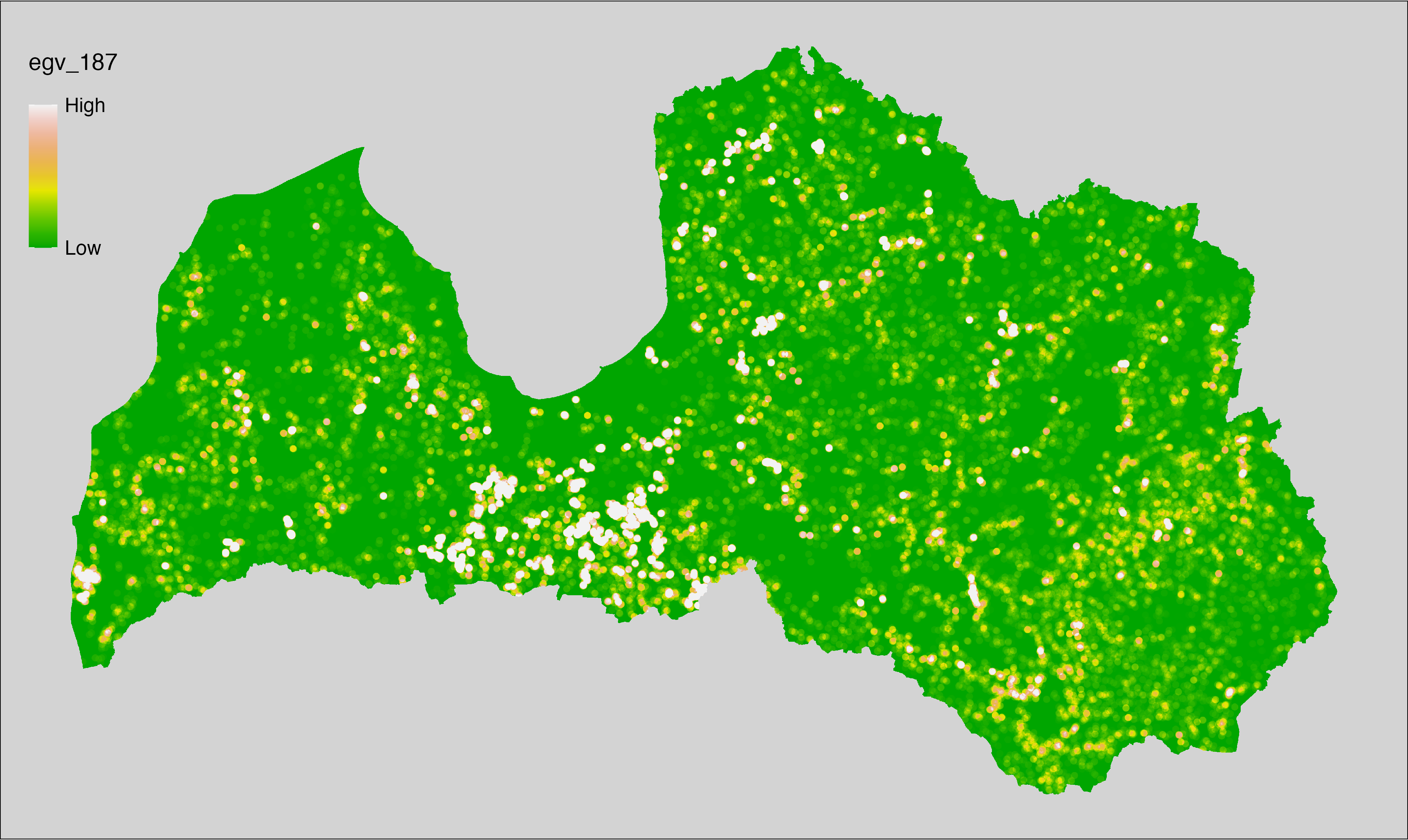
6.188 FarmlandCrops_CropsHoed_r3000
filename: FarmlandCrops_CropsHoed_r3000.tif
layername: egv_188
English name: Fractional cover of Hoed Crops within the 3 km landscape
Latvian name: Vagu un rušināmkultūru platības īpatsvars 3 km ainavā
Procedure: The cover fraction within a radius of 3000 m around the analysis grid cell
is calculated as the area-weighted sum of the analysis cells inside
the buffer, using the workflow egvtools::radius_function(). During the calculation of the landscape
metric, inverse distance weighted (power = 2) gap filling on the output is
applied to ensure no missing values at the edges. Then the layer is
rewritten to set its name. Finally, the layer is standardised by
subtracting the arithmetic mean and dividing by the root mean squared error.
Code
# libs ----
if(!require(terra)) {install.packages("terra"); require(terra)}
if(!require(egvtools)) {remotes::install_github("aavotins/egvtools"); require(egvtools)}
# Templates -----
template100=rast("./Templates/TemplateRasters/LV100m_10km.tif")
# radii ----
radius_function(
kvadrati_path = "./Templates/TemplateGrids/tiles/",
radii_path = "./Templates/TemplateGridPoints/tiles/",
tikls100_path = "./Templates/TemplateGrids/tikls100_sauzeme.parquet",
template_path = "./Templates/TemplateRasters/LV100m_10km.tif",
input_layers = c("./RasterGrids_100m/2024/RAW/FarmlandCrops_CropsHoed_cell.tif"),
layer_prefixes = c("FarmlandCrops_CropsHoed"),
output_dir = "./RasterGrids_100m/2024/RAW/",
n_workers = 6,
radii = c("r3000"),
radius_mode = "sparse",
extract_fun = "mean",
fill_missing = TRUE,
IDW_weight = 2,
future_max_size = 40 * 1024^3)
# FarmlandCrops_CropsHoed_r3000.tif egv_188 ----
slanis=rast("./RasterGrids_100m/2024/RAW/FarmlandCrops_CropsHoed_r3000.tif")
names(slanis)="egv_188"
slanis2=project(slanis,template100)
writeRaster(slanis2,
"./RasterGrids_100m/2024/RAW/FarmlandCrops_CropsHoed_r3000.tif",
overwrite=TRUE)
# standardisation ----
if(!require(terra)) {install.packages("terra"); require(terra)}
if(!require(tidyverse)) {install.packages("tidyverse"); require(tidyverse)}
nosaukums="FarmlandCrops_CropsHoed_r3000.tif"
ielasisanas_cels=paste0("./RasterGrids_100m/2024/RAW/",nosaukums)
saglabasanas_cels=paste0("./RasterGrids_100m/2024/Scaled/",nosaukums)
slanis=rast(ielasisanas_cels)
videjais=global(slanis,fun="mean",na.rm=TRUE)
centrets=slanis-videjais[,1]
standartnovirze=terra::global(centrets,fun="rms",na.rm=TRUE)
merogots=centrets/standartnovirze[,1]
writeRaster(merogots,
filename=saglabasanas_cels,
overwrite=TRUE)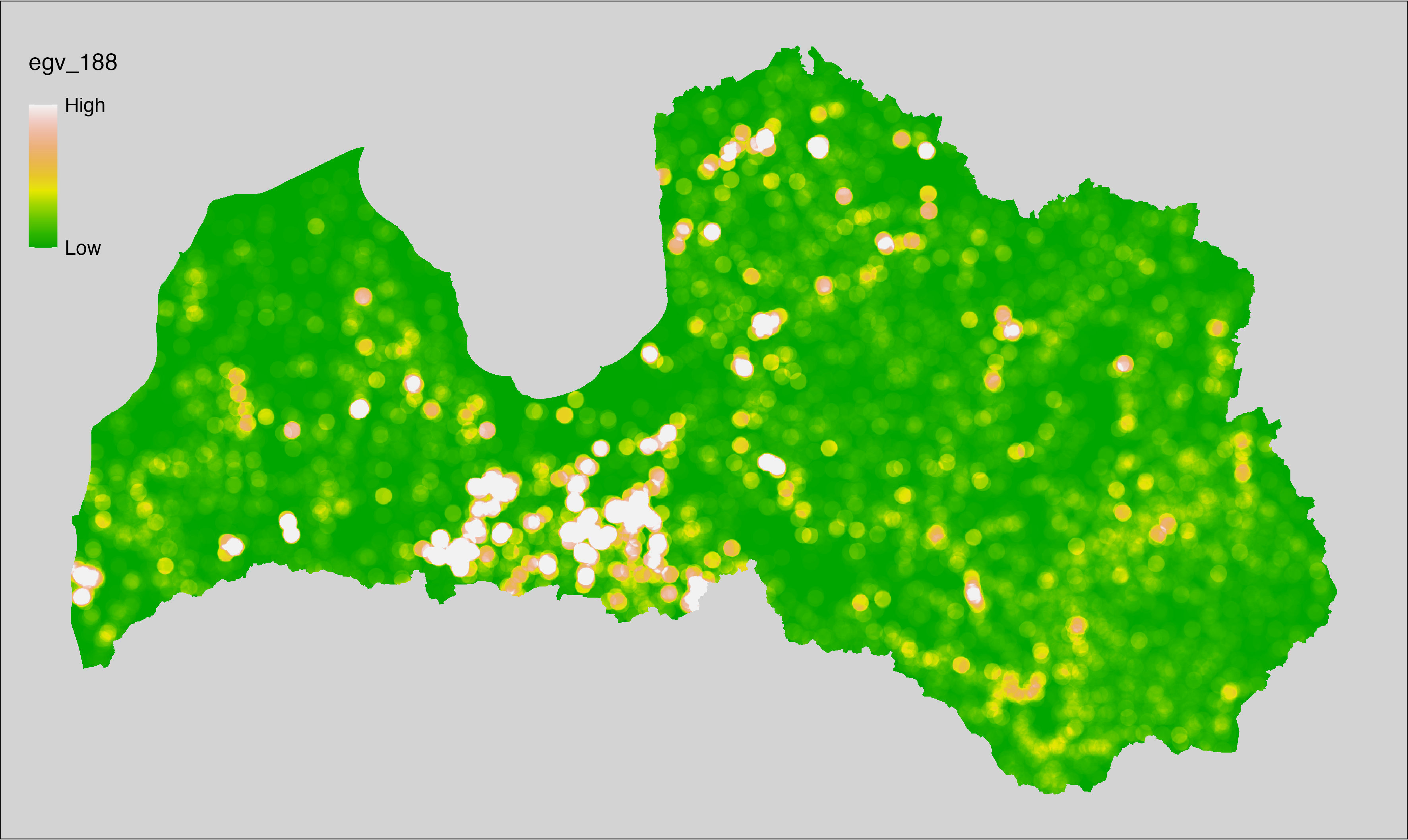
6.189 FarmlandCrops_CropsHoed_r10000
filename: FarmlandCrops_CropsHoed_r10000.tif
layername: egv_189
English name: Fractional cover of Hoed Crops within the 10 km landscape
Latvian name: Vagu un rušināmkultūru platības īpatsvars 10 km ainavā
Procedure: The cover fraction within a radius of 10000 m around the analysis grid cell
is calculated as the area-weighted sum of the analysis cells inside
the buffer, using the workflow egvtools::radius_function(). During the calculation of the landscape
metric, inverse distance weighted (power = 2) gap filling on the output is
applied to ensure no missing values at the edges. Then the layer is
rewritten to set its name. Finally, the layer is standardised by
subtracting the arithmetic mean and dividing by the root mean squared error.
Code
# libs ----
if(!require(terra)) {install.packages("terra"); require(terra)}
if(!require(egvtools)) {remotes::install_github("aavotins/egvtools"); require(egvtools)}
# Templates -----
template100=rast("./Templates/TemplateRasters/LV100m_10km.tif")
# radii ----
radius_function(
kvadrati_path = "./Templates/TemplateGrids/tiles/",
radii_path = "./Templates/TemplateGridPoints/tiles/",
tikls100_path = "./Templates/TemplateGrids/tikls100_sauzeme.parquet",
template_path = "./Templates/TemplateRasters/LV100m_10km.tif",
input_layers = c("./RasterGrids_100m/2024/RAW/FarmlandCrops_CropsHoed_cell.tif"),
layer_prefixes = c("FarmlandCrops_CropsHoed"),
output_dir = "./RasterGrids_100m/2024/RAW/",
n_workers = 6,
radii = c("r10000"),
radius_mode = "sparse",
extract_fun = "mean",
fill_missing = TRUE,
IDW_weight = 2,
future_max_size = 40 * 1024^3)
# FarmlandCrops_CropsHoed_r10000.tif egv_189 ----
slanis=rast("./RasterGrids_100m/2024/RAW/FarmlandCrops_CropsHoed_r10000.tif")
names(slanis)="egv_189"
slanis2=project(slanis,template100)
writeRaster(slanis2,
"./RasterGrids_100m/2024/RAW/FarmlandCrops_CropsHoed_r10000.tif",
overwrite=TRUE)
# standardisation ----
if(!require(terra)) {install.packages("terra"); require(terra)}
if(!require(tidyverse)) {install.packages("tidyverse"); require(tidyverse)}
nosaukums="FarmlandCrops_CropsHoed_r10000.tif"
ielasisanas_cels=paste0("./RasterGrids_100m/2024/RAW/",nosaukums)
saglabasanas_cels=paste0("./RasterGrids_100m/2024/Scaled/",nosaukums)
slanis=rast(ielasisanas_cels)
videjais=global(slanis,fun="mean",na.rm=TRUE)
centrets=slanis-videjais[,1]
standartnovirze=terra::global(centrets,fun="rms",na.rm=TRUE)
merogots=centrets/standartnovirze[,1]
writeRaster(merogots,
filename=saglabasanas_cels,
overwrite=TRUE)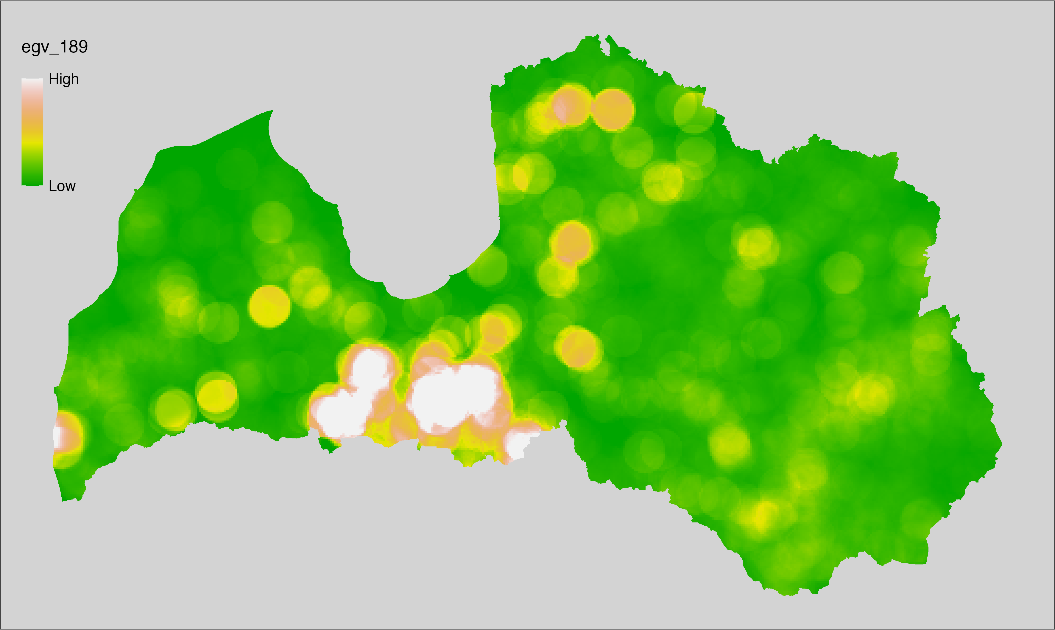
6.190 FarmlandCrops_CropsOther_cell
filename: FarmlandCrops_CropsOther_cell.tif
layername: egv_190
English name: Fractional cover of Other Crops within the analysis cell (1 ha)
Latvian name: Citu lauksaimniecības kultūraugu aramzemēs platības īpatsvars analīzes šūnā (1 ha)
Procedure: First, agricultural parcels with otherwise not differentiated
crops are selected from the Rural Support Service’s information on declared
fields. These geometries are then rasterised to input resolution,
ensuring value 1 at the polygon locations and value 0 elsewhere. Rasterisation is performed using the workflow egvtools::polygon2input(). Once rasterised, the layer is aggregated to EGV
resolution using the workflow egvtools::input2egv(), which calculates the arithmetic mean and thus
results in a cover fraction. During aggregation, inverse
distance weighted (power = 2) gap filling on the output is applied to
ensure no missing values at the edges. Finally, the layer is standardised
by subtracting the arithmetic mean and dividing by the root mean squared error.
Code
# libs ----
if(!require(egvtools)) {remotes::install_github("aavotins/egvtools"); require(egvtools)}
if(!require(terra)) {install.packages("terra"); require(terra)}
if(!require(sf)) {install.packages("sf"); require(sf)}
if(!require(tidyverse)) {install.packages("tidyverse"); require(tidyverse)}
if(!require(sfarrow)) {install.packages("sfarrow"); require(sfarrow)}
if(!require(readxl)) {install.packages("readxl"); require(readxl)}
if(!require(raster)) {install.packages("raster"); require(raster)}
if(!require(fasterize)) {install.packages("fasterize"); require(fasterize)}
# templates ----
template100=rast("./Templates/TemplateRasters/LV100m_10km.tif")
template10=rast("./Templates/TemplateRasters/LV10m_10km.tif")
rastrs10=raster(template10)
nulls10=rast("./Templates/TemplateRasters/nulls_LV10m_10km.tif")
nulls100=rast("./Templates/TemplateRasters/nulls_LV100m_10km.tif")
# codes ----
kodi=read_excel("./Geodata/2024/LAD/KulturuKodi_2024.xlsx")
kodi$kods=as.character(kodi$kods)
# LAD ----
lad=sfarrow::st_read_parquet("./Geodata/2024/LAD/Lauki_2024.parquet")
lad$yes=1
lad=lad %>%
left_join(kodi,by=c("PRODUCT_CODE"="kods"))
# simple landscape ----
simple_landscape=rast("RasterGrids_10m/2024/Ainava_vienk_mask.tif")
# FarmlandCrops_CropsOther_cell.tif egv_190 ----
dati=lad %>%
filter(str_detect(SDM_grupa_sakums,"citur neie"))
table(dati$SDM_grupa_sakums,useNA="always")
p2i_rez=egvtools::polygon2input(vector_data = dati,
template_path = "./Templates/TemplateRasters/LV10m_10km.tif",
out_path = "./RasterGrids_10m/2024/",
file_name = "FarmlandCrops_CropsOther_input.tif",
value_field = "yes",
prepare=FALSE,
background_raster = "./Templates/TemplateRasters/nulls_LV10m_10km.tif",
plot_result = TRUE)
p2i_rez
i2e_rez=egvtools::input2egv(input=paste0("./RasterGrids_10m/2024/",
"FarmlandCrops_CropsOther_input.tif"),
egv_template= "./Templates/TemplateRasters/LV100m_10km.tif",
summary_function = "average",
missing_job = "FillOutput",
outlocation = "./RasterGrids_100m/2024/RAW/",
outfilename = "FarmlandCrops_CropsOther_cell.tif",
layername = "egv_190",
idw_weight = 2,
plot_gaps = FALSE,plot_final = TRUE)
i2e_rez
rm(p2i_rez)
rm(i2e_rez)
rm(dati)
unlink("./RasterGrids_10m/2024/FarmlandCrops_CropsOther_input.tif")
# standardisation ----
if(!require(terra)) {install.packages("terra"); require(terra)}
if(!require(tidyverse)) {install.packages("tidyverse"); require(tidyverse)}
nosaukums="FarmlandCrops_CropsOther_cell.tif"
ielasisanas_cels=paste0("./RasterGrids_100m/2024/RAW/",nosaukums)
saglabasanas_cels=paste0("./RasterGrids_100m/2024/Scaled/",nosaukums)
slanis=rast(ielasisanas_cels)
videjais=global(slanis,fun="mean",na.rm=TRUE)
centrets=slanis-videjais[,1]
standartnovirze=terra::global(centrets,fun="rms",na.rm=TRUE)
merogots=centrets/standartnovirze[,1]
writeRaster(merogots,
filename=saglabasanas_cels,
overwrite=TRUE)
6.191 FarmlandCrops_CropsOther_r500
filename: FarmlandCrops_CropsOther_r500.tif
layername: egv_191
English name: Fractional cover of Other Crops within the 0.5 km landscape
Latvian name: Citu lauksaimniecības kultūraugu aramzemēs platības īpatsvars 0,5 km ainavā
Procedure: The cover fraction within a radius of 500 m around the analysis grid cell is
calculated as the area-weighted sum of the analysis cells inside the
buffer, using the workflow egvtools::radius_function(). During the calculation of the landscape metric,
inverse distance weighted (power = 2) gap filling on the output is applied
to ensure no missing values at the edges. Then the layer is rewritten to set
its name. Finally, the layer is standardised by subtracting the arithmetic
mean and dividing by the root mean squared error.
Code
# libs ----
if(!require(terra)) {install.packages("terra"); require(terra)}
if(!require(egvtools)) {remotes::install_github("aavotins/egvtools"); require(egvtools)}
# Templates -----
template100=rast("./Templates/TemplateRasters/LV100m_10km.tif")
# radii ----
radius_function(
kvadrati_path = "./Templates/TemplateGrids/tiles/",
radii_path = "./Templates/TemplateGridPoints/tiles/",
tikls100_path = "./Templates/TemplateGrids/tikls100_sauzeme.parquet",
template_path = "./Templates/TemplateRasters/LV100m_10km.tif",
input_layers = c("./RasterGrids_100m/2024/RAW/FarmlandCrops_CropsOther_cell.tif"),
layer_prefixes = c("FarmlandCrops_CropsOther"),
output_dir = "./RasterGrids_100m/2024/RAW/",
n_workers = 6,
radii = c("r500"),
radius_mode = "sparse",
extract_fun = "mean",
fill_missing = TRUE,
IDW_weight = 2,
future_max_size = 40 * 1024^3)
# FarmlandCrops_CropsOther_r500.tif egv_191 ----
slanis=rast("./RasterGrids_100m/2024/RAW/FarmlandCrops_CropsOther_r500.tif")
names(slanis)="egv_191"
slanis2=project(slanis,template100)
writeRaster(slanis2,
"./RasterGrids_100m/2024/RAW/FarmlandCrops_CropsOther_r500.tif",
overwrite=TRUE)
# standardisation ----
if(!require(terra)) {install.packages("terra"); require(terra)}
if(!require(tidyverse)) {install.packages("tidyverse"); require(tidyverse)}
nosaukums="FarmlandCrops_CropsOther_r500.tif"
ielasisanas_cels=paste0("./RasterGrids_100m/2024/RAW/",nosaukums)
saglabasanas_cels=paste0("./RasterGrids_100m/2024/Scaled/",nosaukums)
slanis=rast(ielasisanas_cels)
videjais=global(slanis,fun="mean",na.rm=TRUE)
centrets=slanis-videjais[,1]
standartnovirze=terra::global(centrets,fun="rms",na.rm=TRUE)
merogots=centrets/standartnovirze[,1]
writeRaster(merogots,
filename=saglabasanas_cels,
overwrite=TRUE)
6.192 FarmlandCrops_CropsOther_r1250
filename: FarmlandCrops_CropsOther_r1250.tif
layername: egv_192
English name: Fractional cover of Other Crops within the 1.25 km landscape
Latvian name: Citu lauksaimniecības kultūraugu aramzemēs platības īpatsvars 1,25 km ainavā
Procedure: The cover fraction within a radius of 1250 m around the analysis grid cell
is calculated as the area-weighted sum of the analysis cells inside
the buffer, using the workflow egvtools::radius_function(). During the calculation of the landscape
metric, inverse distance weighted (power = 2) gap filling on the output is
applied to ensure no missing values at the edges. Then the layer is
rewritten to set its name. Finally, the layer is standardised by
subtracting the arithmetic mean and dividing by the root mean squared error.
Code
# libs ----
if(!require(terra)) {install.packages("terra"); require(terra)}
if(!require(egvtools)) {remotes::install_github("aavotins/egvtools"); require(egvtools)}
# Templates -----
template100=rast("./Templates/TemplateRasters/LV100m_10km.tif")
# radii ----
radius_function(
kvadrati_path = "./Templates/TemplateGrids/tiles/",
radii_path = "./Templates/TemplateGridPoints/tiles/",
tikls100_path = "./Templates/TemplateGrids/tikls100_sauzeme.parquet",
template_path = "./Templates/TemplateRasters/LV100m_10km.tif",
input_layers = c("./RasterGrids_100m/2024/RAW/FarmlandCrops_CropsOther_cell.tif"),
layer_prefixes = c("FarmlandCrops_CropsOther"),
output_dir = "./RasterGrids_100m/2024/RAW/",
n_workers = 6,
radii = c("r1250"),
radius_mode = "sparse",
extract_fun = "mean",
fill_missing = TRUE,
IDW_weight = 2,
future_max_size = 40 * 1024^3)
# FarmlandCrops_CropsOther_r1250.tif egv_192 ----
slanis=rast("./RasterGrids_100m/2024/RAW/FarmlandCrops_CropsOther_r1250.tif")
names(slanis)="egv_192"
slanis2=project(slanis,template100)
writeRaster(slanis2,
"./RasterGrids_100m/2024/RAW/FarmlandCrops_CropsOther_r1250.tif",
overwrite=TRUE)
# standardisation ----
if(!require(terra)) {install.packages("terra"); require(terra)}
if(!require(tidyverse)) {install.packages("tidyverse"); require(tidyverse)}
nosaukums="FarmlandCrops_CropsOther_r1250.tif"
ielasisanas_cels=paste0("./RasterGrids_100m/2024/RAW/",nosaukums)
saglabasanas_cels=paste0("./RasterGrids_100m/2024/Scaled/",nosaukums)
slanis=rast(ielasisanas_cels)
videjais=global(slanis,fun="mean",na.rm=TRUE)
centrets=slanis-videjais[,1]
standartnovirze=terra::global(centrets,fun="rms",na.rm=TRUE)
merogots=centrets/standartnovirze[,1]
writeRaster(merogots,
filename=saglabasanas_cels,
overwrite=TRUE)
6.193 FarmlandCrops_CropsOther_r3000
filename: FarmlandCrops_CropsOther_r3000.tif
layername: egv_193
English name: Fractional cover of Other Crops within the 3 km landscape
Latvian name: Citu lauksaimniecības kultūraugu aramzemēs platības īpatsvars 3 km ainavā
Procedure: The cover fraction within a radius of 3000 m around the analysis grid cell
is calculated as the area-weighted sum of the analysis cells inside
the buffer, using the workflow egvtools::radius_function(). During the calculation of the landscape
metric, inverse distance weighted (power = 2) gap filling on the output is
applied to ensure no missing values at the edges. Then the layer is
rewritten to set its name. Finally, the layer is standardised by
subtracting the arithmetic mean and dividing by the root mean squared error.
Code
# libs ----
if(!require(terra)) {install.packages("terra"); require(terra)}
if(!require(egvtools)) {remotes::install_github("aavotins/egvtools"); require(egvtools)}
# Templates -----
template100=rast("./Templates/TemplateRasters/LV100m_10km.tif")
# radii ----
radius_function(
kvadrati_path = "./Templates/TemplateGrids/tiles/",
radii_path = "./Templates/TemplateGridPoints/tiles/",
tikls100_path = "./Templates/TemplateGrids/tikls100_sauzeme.parquet",
template_path = "./Templates/TemplateRasters/LV100m_10km.tif",
input_layers = c("./RasterGrids_100m/2024/RAW/FarmlandCrops_CropsOther_cell.tif"),
layer_prefixes = c("FarmlandCrops_CropsOther"),
output_dir = "./RasterGrids_100m/2024/RAW/",
n_workers = 6,
radii = c("r3000"),
radius_mode = "sparse",
extract_fun = "mean",
fill_missing = TRUE,
IDW_weight = 2,
future_max_size = 40 * 1024^3)
# FarmlandCrops_CropsOther_r3000.tif egv_193 ----
slanis=rast("./RasterGrids_100m/2024/RAW/FarmlandCrops_CropsOther_r3000.tif")
names(slanis)="egv_193"
slanis2=project(slanis,template100)
writeRaster(slanis2,
"./RasterGrids_100m/2024/RAW/FarmlandCrops_CropsOther_r3000.tif",
overwrite=TRUE)
# standardisation ----
if(!require(terra)) {install.packages("terra"); require(terra)}
if(!require(tidyverse)) {install.packages("tidyverse"); require(tidyverse)}
nosaukums="FarmlandCrops_CropsOther_r3000.tif"
ielasisanas_cels=paste0("./RasterGrids_100m/2024/RAW/",nosaukums)
saglabasanas_cels=paste0("./RasterGrids_100m/2024/Scaled/",nosaukums)
slanis=rast(ielasisanas_cels)
videjais=global(slanis,fun="mean",na.rm=TRUE)
centrets=slanis-videjais[,1]
standartnovirze=terra::global(centrets,fun="rms",na.rm=TRUE)
merogots=centrets/standartnovirze[,1]
writeRaster(merogots,
filename=saglabasanas_cels,
overwrite=TRUE)
6.194 FarmlandCrops_CropsOther_r10000
filename: FarmlandCrops_CropsOther_r10000.tif
layername: egv_194
English name: Fractional cover of Other Crops within the 10 km landscape
Latvian name: Citu lauksaimniecības kultūraugu aramzemēs platības īpatsvars 10 km ainavā
Procedure: The cover fraction within a radius of 10000 m around the analysis grid cell
is calculated as the area-weighted sum of the analysis cells inside
the buffer, using the workflow egvtools::radius_function(). During the calculation of the landscape
metric, inverse distance weighted (power = 2) gap filling on the output is
applied to ensure no missing values at the edges. Then the layer is
rewritten to set its name. Finally, the layer is standardised by
subtracting the arithmetic mean and dividing by the root mean squared error.
Code
# libs ----
if(!require(terra)) {install.packages("terra"); require(terra)}
if(!require(egvtools)) {remotes::install_github("aavotins/egvtools"); require(egvtools)}
# Templates -----
template100=rast("./Templates/TemplateRasters/LV100m_10km.tif")
# radii ----
radius_function(
kvadrati_path = "./Templates/TemplateGrids/tiles/",
radii_path = "./Templates/TemplateGridPoints/tiles/",
tikls100_path = "./Templates/TemplateGrids/tikls100_sauzeme.parquet",
template_path = "./Templates/TemplateRasters/LV100m_10km.tif",
input_layers = c("./RasterGrids_100m/2024/RAW/FarmlandCrops_CropsOther_cell.tif"),
layer_prefixes = c("FarmlandCrops_CropsOther"),
output_dir = "./RasterGrids_100m/2024/RAW/",
n_workers = 6,
radii = c("r10000"),
radius_mode = "sparse",
extract_fun = "mean",
fill_missing = TRUE,
IDW_weight = 2,
future_max_size = 40 * 1024^3)
# FarmlandCrops_CropsOther_r10000.tif egv_194 ----
slanis=rast("./RasterGrids_100m/2024/RAW/FarmlandCrops_CropsOther_r10000.tif")
names(slanis)="egv_194"
slanis2=project(slanis,template100)
writeRaster(slanis2,
"./RasterGrids_100m/2024/RAW/FarmlandCrops_CropsOther_r10000.tif",
overwrite=TRUE)
# standardisation ----
if(!require(terra)) {install.packages("terra"); require(terra)}
if(!require(tidyverse)) {install.packages("tidyverse"); require(tidyverse)}
nosaukums="FarmlandCrops_CropsOther_r10000.tif"
ielasisanas_cels=paste0("./RasterGrids_100m/2024/RAW/",nosaukums)
saglabasanas_cels=paste0("./RasterGrids_100m/2024/Scaled/",nosaukums)
slanis=rast(ielasisanas_cels)
videjais=global(slanis,fun="mean",na.rm=TRUE)
centrets=slanis-videjais[,1]
standartnovirze=terra::global(centrets,fun="rms",na.rm=TRUE)
merogots=centrets/standartnovirze[,1]
writeRaster(merogots,
filename=saglabasanas_cels,
overwrite=TRUE)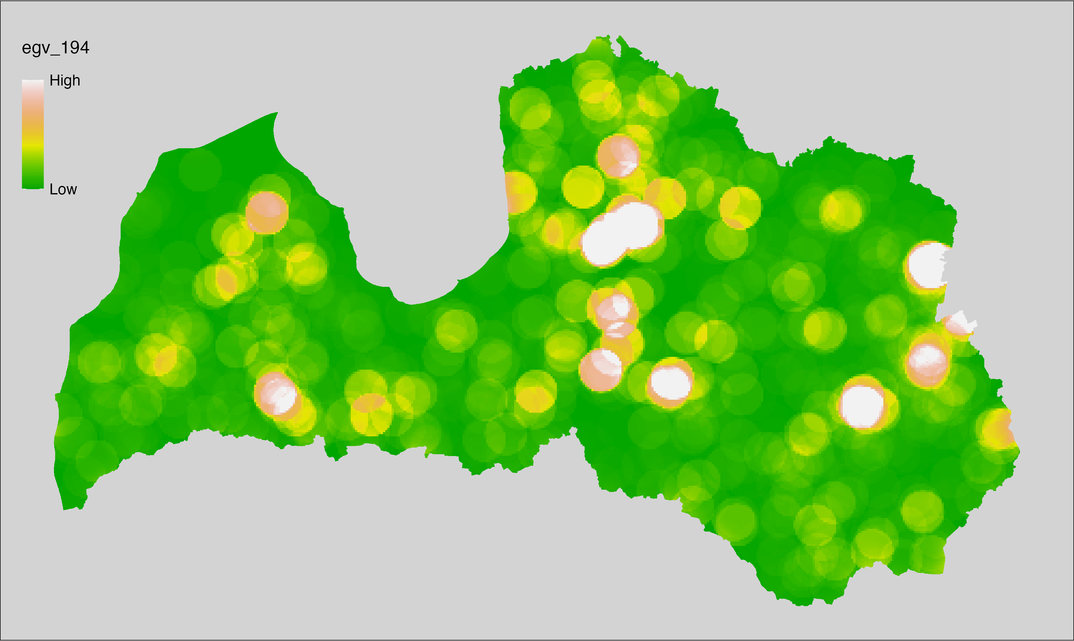
6.195 FarmlandCrops_CropsSpring_cell
filename: FarmlandCrops_CropsSpring_cell.tif
layername: egv_195
English name: Fractional cover of Spring Sown Crops within the analysis cell (1 ha)
Latvian name: Vasarāju aramzemēs platības īpatsvars analīzes šūnā (1 ha)
Procedure: First, agricultural parcels declared as spring sown crops
are selected from the Rural Support Service’s information on declared
fields. These geometries are then rasterised to input resolution,
ensuring value 1 at the polygon locations and value 0 elsewhere. Rasterisation is performed using the workflow egvtools::polygon2input(). Once rasterised, the layer is aggregated to EGV
resolution using the workflow egvtools::input2egv(), which calculates the arithmetic mean and thus
results in a cover fraction. During aggregation, inverse
distance weighted (power = 2) gap filling on the output is applied to
ensure no missing values at the edges. Finally, the layer is standardised
by subtracting the arithmetic mean and dividing by the root mean squared error.
Code
# libs ----
if(!require(egvtools)) {remotes::install_github("aavotins/egvtools"); require(egvtools)}
if(!require(terra)) {install.packages("terra"); require(terra)}
if(!require(sf)) {install.packages("sf"); require(sf)}
if(!require(tidyverse)) {install.packages("tidyverse"); require(tidyverse)}
if(!require(sfarrow)) {install.packages("sfarrow"); require(sfarrow)}
if(!require(readxl)) {install.packages("readxl"); require(readxl)}
if(!require(raster)) {install.packages("raster"); require(raster)}
if(!require(fasterize)) {install.packages("fasterize"); require(fasterize)}
# templates ----
template100=rast("./Templates/TemplateRasters/LV100m_10km.tif")
template10=rast("./Templates/TemplateRasters/LV10m_10km.tif")
rastrs10=raster(template10)
nulls10=rast("./Templates/TemplateRasters/nulls_LV10m_10km.tif")
nulls100=rast("./Templates/TemplateRasters/nulls_LV100m_10km.tif")
# codes ----
kodi=read_excel("./Geodata/2024/LAD/KulturuKodi_2024.xlsx")
kodi$kods=as.character(kodi$kods)
# LAD ----
lad=sfarrow::st_read_parquet("./Geodata/2024/LAD/Lauki_2024.parquet")
lad$yes=1
lad=lad %>%
left_join(kodi,by=c("PRODUCT_CODE"="kods"))
# simple landscape ----
simple_landscape=rast("RasterGrids_10m/2024/Ainava_vienk_mask.tif")
# FarmlandCrops_CropsSpring_cell.tif egv_195 ----
dati=lad %>%
filter(str_detect(SDM_grupa_sakums,"labība-vasarāji"))
table(dati$SDM_grupa_sakums,useNA="always")
p2i_rez=egvtools::polygon2input(vector_data = dati,
template_path = "./Templates/TemplateRasters/LV10m_10km.tif",
out_path = "./RasterGrids_10m/2024/",
file_name = "FarmlandCrops_CropsSpring_input.tif",
value_field = "yes",
prepare=FALSE,
background_raster = "./Templates/TemplateRasters/nulls_LV10m_10km.tif",
plot_result = TRUE)
p2i_rez
i2e_rez=egvtools::input2egv(input=paste0("./RasterGrids_10m/2024/",
"FarmlandCrops_CropsSpring_input.tif"),
egv_template= "./Templates/TemplateRasters/LV100m_10km.tif",
summary_function = "average",
missing_job = "FillOutput",
outlocation = "./RasterGrids_100m/2024/RAW/",
outfilename = "FarmlandCrops_CropsSpring_cell.tif",
layername = "egv_195",
idw_weight = 2,
plot_gaps = FALSE,plot_final = TRUE)
i2e_rez
rm(p2i_rez)
rm(i2e_rez)
rm(dati)
unlink("./RasterGrids_10m/2024/FarmlandCrops_CropsSpring_input.tif")
# standardisation ----
if(!require(terra)) {install.packages("terra"); require(terra)}
if(!require(tidyverse)) {install.packages("tidyverse"); require(tidyverse)}
nosaukums="FarmlandCrops_CropsSpring_cell.tif"
ielasisanas_cels=paste0("./RasterGrids_100m/2024/RAW/",nosaukums)
saglabasanas_cels=paste0("./RasterGrids_100m/2024/Scaled/",nosaukums)
slanis=rast(ielasisanas_cels)
videjais=global(slanis,fun="mean",na.rm=TRUE)
centrets=slanis-videjais[,1]
standartnovirze=terra::global(centrets,fun="rms",na.rm=TRUE)
merogots=centrets/standartnovirze[,1]
writeRaster(merogots,
filename=saglabasanas_cels,
overwrite=TRUE)
6.196 FarmlandCrops_CropsSpring_r500
filename: FarmlandCrops_CropsSpring_r500.tif
layername: egv_196
English name: Fractional cover of Spring Sown Crops within the 0.5 km landscape
Latvian name: Vasarāju aramzemēs platības īpatsvars 0,5 km ainavā
Procedure: The cover fraction within a radius of 500 m around the analysis grid cell is
calculated as the area-weighted sum of the analysis cells inside the
buffer, using the workflow egvtools::radius_function(). During the calculation of the landscape metric,
inverse distance weighted (power = 2) gap filling on the output is applied
to ensure no missing values at the edges. Then the layer is rewritten to set
its name. Finally, the layer is standardised by subtracting the arithmetic
mean and dividing by the root mean squared error.
Code
# libs ----
if(!require(terra)) {install.packages("terra"); require(terra)}
if(!require(egvtools)) {remotes::install_github("aavotins/egvtools"); require(egvtools)}
# Templates -----
template100=rast("./Templates/TemplateRasters/LV100m_10km.tif")
# radii ----
radius_function(
kvadrati_path = "./Templates/TemplateGrids/tiles/",
radii_path = "./Templates/TemplateGridPoints/tiles/",
tikls100_path = "./Templates/TemplateGrids/tikls100_sauzeme.parquet",
template_path = "./Templates/TemplateRasters/LV100m_10km.tif",
input_layers = c("./RasterGrids_100m/2024/RAW/FarmlandCrops_CropsSpring_cell.tif"),
layer_prefixes = c("FarmlandCrops_CropsSpring"),
output_dir = "./RasterGrids_100m/2024/RAW/",
n_workers = 6,
radii = c("r500"),
radius_mode = "sparse",
extract_fun = "mean",
fill_missing = TRUE,
IDW_weight = 2,
future_max_size = 40 * 1024^3)
# FarmlandCrops_CropsSpring_r500.tif egv_196 ----
slanis=rast("./RasterGrids_100m/2024/RAW/FarmlandCrops_CropsSpring_r500.tif")
names(slanis)="egv_196"
slanis2=project(slanis,template100)
writeRaster(slanis2,
"./RasterGrids_100m/2024/RAW/FarmlandCrops_CropsSpring_r500.tif",
overwrite=TRUE)
# standardisation ----
if(!require(terra)) {install.packages("terra"); require(terra)}
if(!require(tidyverse)) {install.packages("tidyverse"); require(tidyverse)}
nosaukums="FarmlandCrops_CropsSpring_r500.tif"
ielasisanas_cels=paste0("./RasterGrids_100m/2024/RAW/",nosaukums)
saglabasanas_cels=paste0("./RasterGrids_100m/2024/Scaled/",nosaukums)
slanis=rast(ielasisanas_cels)
videjais=global(slanis,fun="mean",na.rm=TRUE)
centrets=slanis-videjais[,1]
standartnovirze=terra::global(centrets,fun="rms",na.rm=TRUE)
merogots=centrets/standartnovirze[,1]
writeRaster(merogots,
filename=saglabasanas_cels,
overwrite=TRUE)
6.197 FarmlandCrops_CropsSpring_r1250
filename: FarmlandCrops_CropsSpring_r1250.tif
layername: egv_197
English name: Fractional cover of Spring Sown Crops within the 1.25 km landscape
Latvian name: Vasarāju aramzemēs platības īpatsvars 1,25 km ainavā
Procedure: The cover fraction within a radius of 1250 m around the analysis grid cell
is calculated as the area-weighted sum of the analysis cells inside
the buffer, using the workflow egvtools::radius_function(). During the calculation of the landscape
metric, inverse distance weighted (power = 2) gap filling on the output is
applied to ensure no missing values at the edges. Then the layer is
rewritten to set its name. Finally, the layer is standardised by
subtracting the arithmetic mean and dividing by the root mean squared error.
Code
# libs ----
if(!require(terra)) {install.packages("terra"); require(terra)}
if(!require(egvtools)) {remotes::install_github("aavotins/egvtools"); require(egvtools)}
# Templates -----
template100=rast("./Templates/TemplateRasters/LV100m_10km.tif")
# radii ----
radius_function(
kvadrati_path = "./Templates/TemplateGrids/tiles/",
radii_path = "./Templates/TemplateGridPoints/tiles/",
tikls100_path = "./Templates/TemplateGrids/tikls100_sauzeme.parquet",
template_path = "./Templates/TemplateRasters/LV100m_10km.tif",
input_layers = c("./RasterGrids_100m/2024/RAW/FarmlandCrops_CropsSpring_cell.tif"),
layer_prefixes = c("FarmlandCrops_CropsSpring"),
output_dir = "./RasterGrids_100m/2024/RAW/",
n_workers = 6,
radii = c("r1250"),
radius_mode = "sparse",
extract_fun = "mean",
fill_missing = TRUE,
IDW_weight = 2,
future_max_size = 40 * 1024^3)
# FarmlandCrops_CropsSpring_r1250.tif egv_197 ----
slanis=rast("./RasterGrids_100m/2024/RAW/FarmlandCrops_CropsSpring_r1250.tif")
names(slanis)="egv_197"
slanis2=project(slanis,template100)
writeRaster(slanis2,
"./RasterGrids_100m/2024/RAW/FarmlandCrops_CropsSpring_r1250.tif",
overwrite=TRUE)
# standardisation ----
if(!require(terra)) {install.packages("terra"); require(terra)}
if(!require(tidyverse)) {install.packages("tidyverse"); require(tidyverse)}
nosaukums="FarmlandCrops_CropsSpring_r1250.tif"
ielasisanas_cels=paste0("./RasterGrids_100m/2024/RAW/",nosaukums)
saglabasanas_cels=paste0("./RasterGrids_100m/2024/Scaled/",nosaukums)
slanis=rast(ielasisanas_cels)
videjais=global(slanis,fun="mean",na.rm=TRUE)
centrets=slanis-videjais[,1]
standartnovirze=terra::global(centrets,fun="rms",na.rm=TRUE)
merogots=centrets/standartnovirze[,1]
writeRaster(merogots,
filename=saglabasanas_cels,
overwrite=TRUE)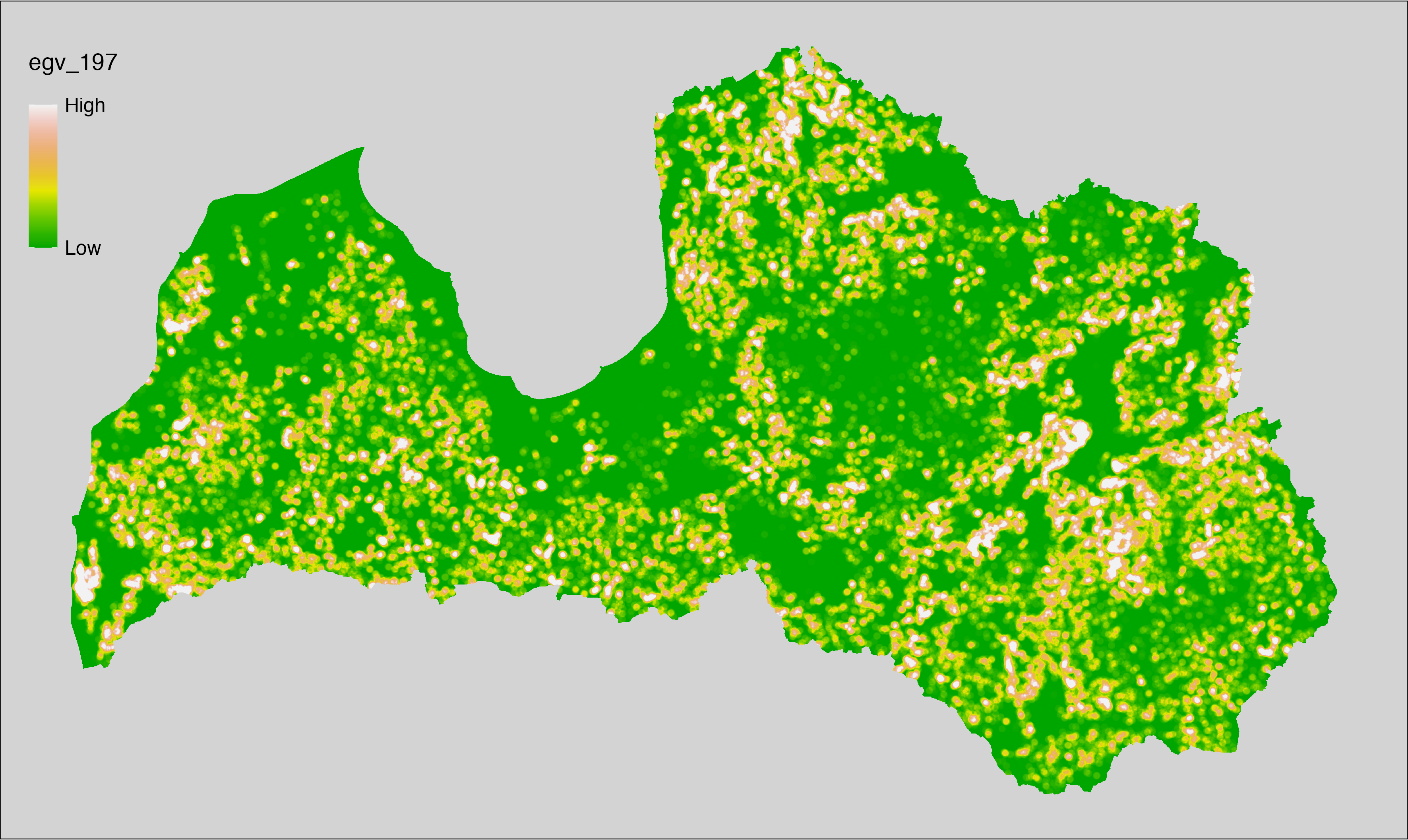
6.198 FarmlandCrops_CropsSpring_r3000
filename: FarmlandCrops_CropsSpring_r3000.tif
layername: egv_198
English name: Fractional cover of Spring Sown Crops within the 3 km landscape
Latvian name: Vasarāju aramzemēs platības īpatsvars 3 km ainavā
Procedure: The cover fraction within a radius of 3000 m around the analysis grid cell
is calculated as the area-weighted sum of the analysis cells inside
the buffer, using the workflow egvtools::radius_function(). During the calculation of the landscape
metric, inverse distance weighted (power = 2) gap filling on the output is
applied to ensure no missing values at the edges. Then the layer is
rewritten to set its name. Finally, the layer is standardised by
subtracting the arithmetic mean and dividing by the root mean squared error.
Code
# libs ----
if(!require(terra)) {install.packages("terra"); require(terra)}
if(!require(egvtools)) {remotes::install_github("aavotins/egvtools"); require(egvtools)}
# Templates -----
template100=rast("./Templates/TemplateRasters/LV100m_10km.tif")
# radii ----
radius_function(
kvadrati_path = "./Templates/TemplateGrids/tiles/",
radii_path = "./Templates/TemplateGridPoints/tiles/",
tikls100_path = "./Templates/TemplateGrids/tikls100_sauzeme.parquet",
template_path = "./Templates/TemplateRasters/LV100m_10km.tif",
input_layers = c("./RasterGrids_100m/2024/RAW/FarmlandCrops_CropsSpring_cell.tif"),
layer_prefixes = c("FarmlandCrops_CropsSpring"),
output_dir = "./RasterGrids_100m/2024/RAW/",
n_workers = 6,
radii = c("r3000"),
radius_mode = "sparse",
extract_fun = "mean",
fill_missing = TRUE,
IDW_weight = 2,
future_max_size = 40 * 1024^3)
# FarmlandCrops_CropsSpring_r3000.tif egv_198 ----
slanis=rast("./RasterGrids_100m/2024/RAW/FarmlandCrops_CropsSpring_r3000.tif")
names(slanis)="egv_198"
slanis2=project(slanis,template100)
writeRaster(slanis2,
"./RasterGrids_100m/2024/RAW/FarmlandCrops_CropsSpring_r3000.tif",
overwrite=TRUE)
# standardisation ----
if(!require(terra)) {install.packages("terra"); require(terra)}
if(!require(tidyverse)) {install.packages("tidyverse"); require(tidyverse)}
nosaukums="FarmlandCrops_CropsSpring_r3000.tif"
ielasisanas_cels=paste0("./RasterGrids_100m/2024/RAW/",nosaukums)
saglabasanas_cels=paste0("./RasterGrids_100m/2024/Scaled/",nosaukums)
slanis=rast(ielasisanas_cels)
videjais=global(slanis,fun="mean",na.rm=TRUE)
centrets=slanis-videjais[,1]
standartnovirze=terra::global(centrets,fun="rms",na.rm=TRUE)
merogots=centrets/standartnovirze[,1]
writeRaster(merogots,
filename=saglabasanas_cels,
overwrite=TRUE)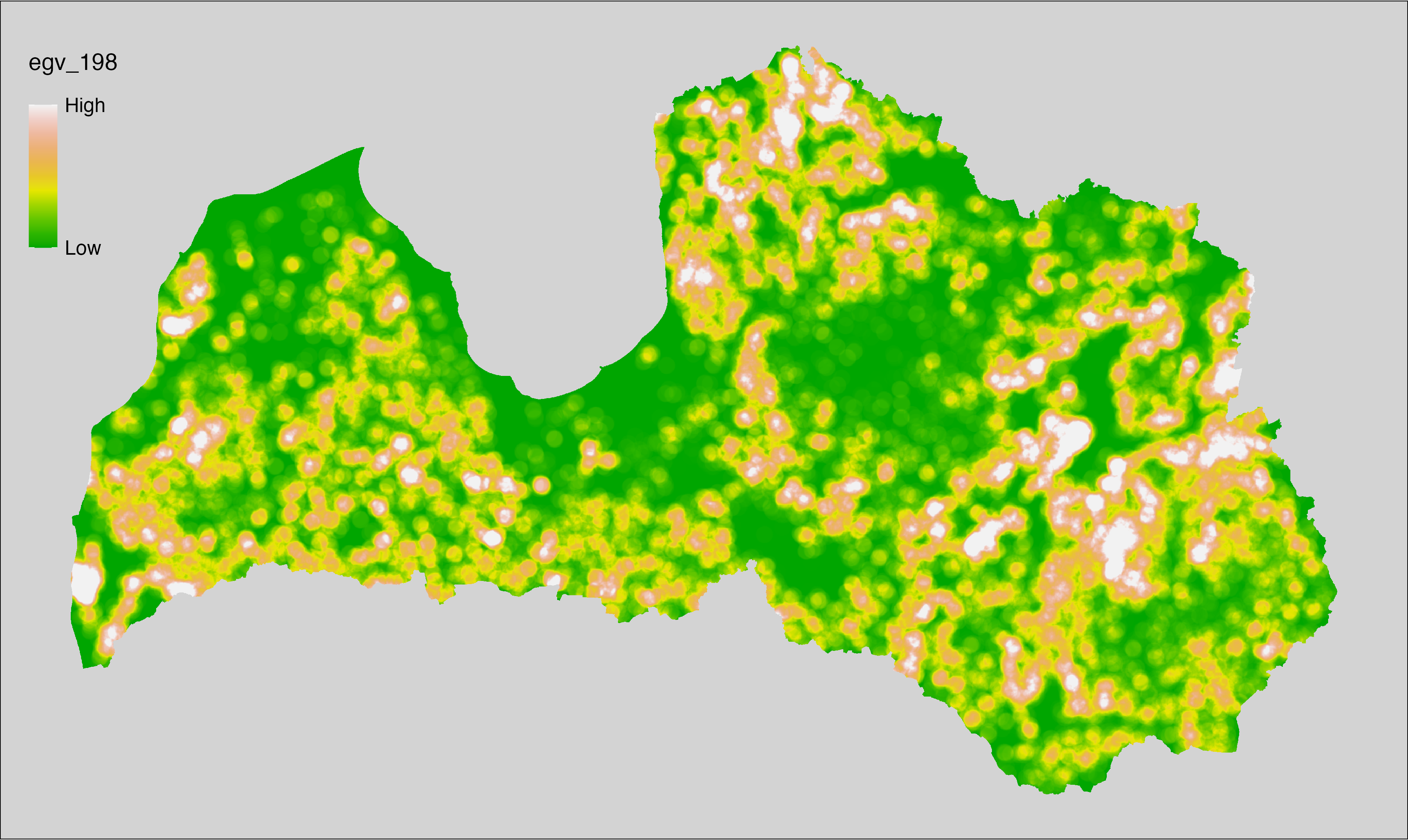
6.199 FarmlandCrops_CropsSpring_r10000
filename: FarmlandCrops_CropsSpring_r10000.tif
layername: egv_199
English name: Fractional cover of Spring Sown Crops within the 10 km landscape
Latvian name: Vasarāju aramzemēs platības īpatsvars 10 km ainavā
Procedure: The cover fraction within a radius of 10000 m around the analysis grid cell
is calculated as the area-weighted sum of the analysis cells inside
the buffer, using the workflow egvtools::radius_function(). During the calculation of the landscape
metric, inverse distance weighted (power = 2) gap filling on the output is
applied to ensure no missing values at the edges. Then the layer is
rewritten to set its name. Finally, the layer is standardised by
subtracting the arithmetic mean and dividing by the root mean squared error.
Code
# libs ----
if(!require(terra)) {install.packages("terra"); require(terra)}
if(!require(egvtools)) {remotes::install_github("aavotins/egvtools"); require(egvtools)}
# Templates -----
template100=rast("./Templates/TemplateRasters/LV100m_10km.tif")
# radii ----
radius_function(
kvadrati_path = "./Templates/TemplateGrids/tiles/",
radii_path = "./Templates/TemplateGridPoints/tiles/",
tikls100_path = "./Templates/TemplateGrids/tikls100_sauzeme.parquet",
template_path = "./Templates/TemplateRasters/LV100m_10km.tif",
input_layers = c("./RasterGrids_100m/2024/RAW/FarmlandCrops_CropsSpring_cell.tif"),
layer_prefixes = c("FarmlandCrops_CropsSpring"),
output_dir = "./RasterGrids_100m/2024/RAW/",
n_workers = 6,
radii = c("r10000"),
radius_mode = "sparse",
extract_fun = "mean",
fill_missing = TRUE,
IDW_weight = 2,
future_max_size = 40 * 1024^3)
# FarmlandCrops_CropsSpring_r10000.tif egv_199 ----
slanis=rast("./RasterGrids_100m/2024/RAW/FarmlandCrops_CropsSpring_r10000.tif")
names(slanis)="egv_199"
slanis2=project(slanis,template100)
writeRaster(slanis2,
"./RasterGrids_100m/2024/RAW/FarmlandCrops_CropsSpring_r10000.tif",
overwrite=TRUE)
# standardisation ----
if(!require(terra)) {install.packages("terra"); require(terra)}
if(!require(tidyverse)) {install.packages("tidyverse"); require(tidyverse)}
nosaukums="FarmlandCrops_CropsSpring_r10000.tif"
ielasisanas_cels=paste0("./RasterGrids_100m/2024/RAW/",nosaukums)
saglabasanas_cels=paste0("./RasterGrids_100m/2024/Scaled/",nosaukums)
slanis=rast(ielasisanas_cels)
videjais=global(slanis,fun="mean",na.rm=TRUE)
centrets=slanis-videjais[,1]
standartnovirze=terra::global(centrets,fun="rms",na.rm=TRUE)
merogots=centrets/standartnovirze[,1]
writeRaster(merogots,
filename=saglabasanas_cels,
overwrite=TRUE)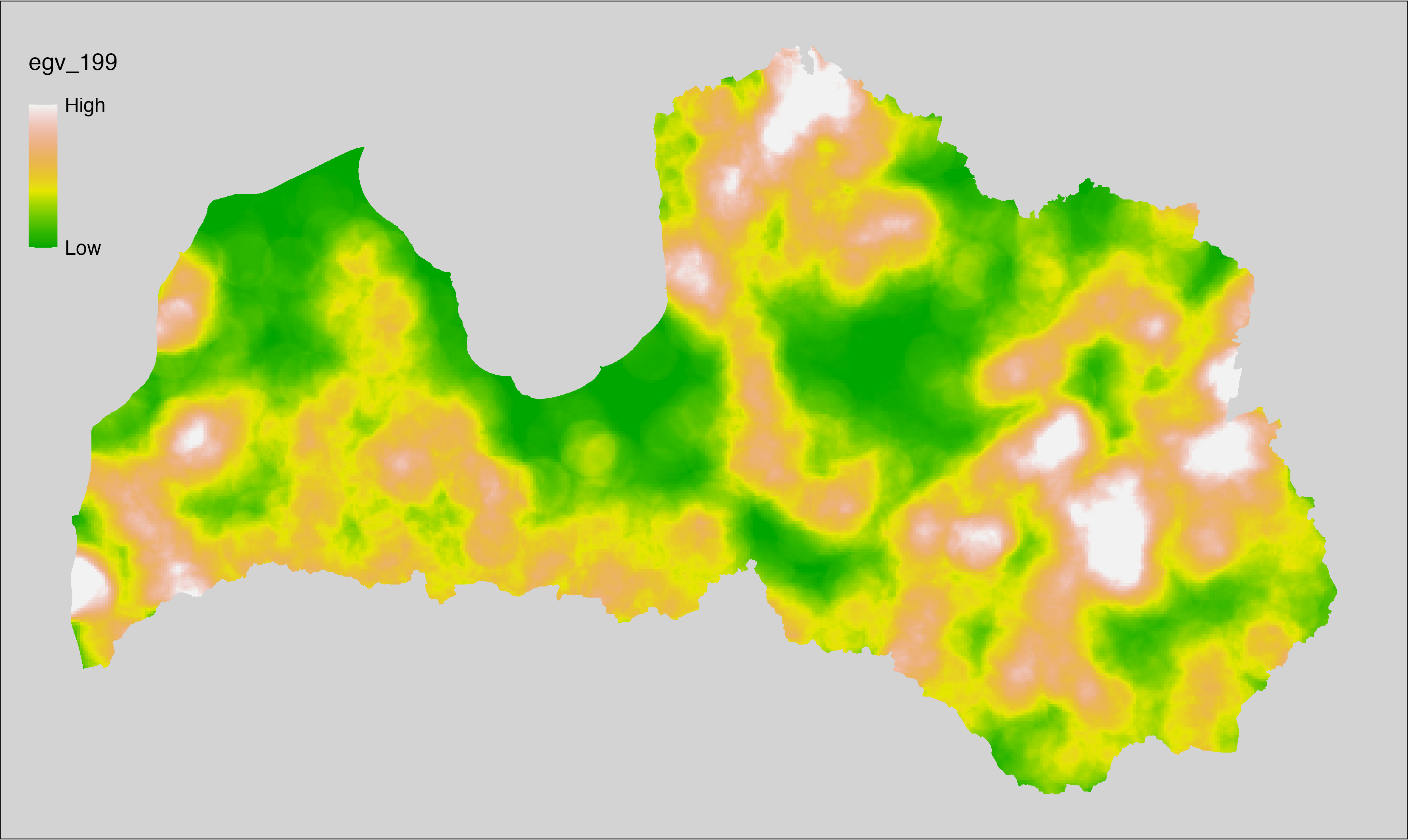
6.200 FarmlandCrops_CropsWinter_cell
filename: FarmlandCrops_CropsWinter_cell.tif
layername: egv_200
English name: Fractional cover of Winter Crops within the analysis cell (1 ha)
Latvian name: Ziemāju aramzemēs platības īpatsvars analīzes šūnā (1 ha)
Procedure: First, agricultural parcels declared as winter crops are
selected from the Rural Support Service’s information on declared
fields. These geometries are then rasterised to input resolution,
ensuring value 1 at the polygon locations and value 0 elsewhere. Rasterisation is performed using the workflow egvtools::polygon2input(). Once rasterised, the layer is aggregated to EGV
resolution using the workflow egvtools::input2egv(), which calculates the arithmetic mean and thus
results in a cover fraction. During aggregation, inverse
distance weighted (power = 2) gap filling on the output is applied to
ensure no missing values at the edges. Finally, the layer is standardised
by subtracting the arithmetic mean and dividing by the root mean squared error.
Code
# libs ----
if(!require(egvtools)) {remotes::install_github("aavotins/egvtools"); require(egvtools)}
if(!require(terra)) {install.packages("terra"); require(terra)}
if(!require(sf)) {install.packages("sf"); require(sf)}
if(!require(tidyverse)) {install.packages("tidyverse"); require(tidyverse)}
if(!require(sfarrow)) {install.packages("sfarrow"); require(sfarrow)}
if(!require(readxl)) {install.packages("readxl"); require(readxl)}
if(!require(raster)) {install.packages("raster"); require(raster)}
if(!require(fasterize)) {install.packages("fasterize"); require(fasterize)}
# templates ----
template100=rast("./Templates/TemplateRasters/LV100m_10km.tif")
template10=rast("./Templates/TemplateRasters/LV10m_10km.tif")
rastrs10=raster(template10)
nulls10=rast("./Templates/TemplateRasters/nulls_LV10m_10km.tif")
nulls100=rast("./Templates/TemplateRasters/nulls_LV100m_10km.tif")
# codes ----
kodi=read_excel("./Geodata/2024/LAD/KulturuKodi_2024.xlsx")
kodi$kods=as.character(kodi$kods)
# LAD ----
lad=sfarrow::st_read_parquet("./Geodata/2024/LAD/Lauki_2024.parquet")
lad$yes=1
lad=lad %>%
left_join(kodi,by=c("PRODUCT_CODE"="kods"))
# simple landscape ----
simple_landscape=rast("RasterGrids_10m/2024/Ainava_vienk_mask.tif")
# FarmlandCrops_CropsWinter_cell.tif egv_200 ----
dati=lad %>%
filter(str_detect(SDM_grupa_sakums,"labība-ziemāji"))
table(dati$SDM_grupa_sakums,useNA="always")
p2i_rez=egvtools::polygon2input(vector_data = dati,
template_path = "./Templates/TemplateRasters/LV10m_10km.tif",
out_path = "./RasterGrids_10m/2024/",
file_name = "FarmlandCrops_CropsWinter_input.tif",
value_field = "yes",
prepare=FALSE,
background_raster = "./Templates/TemplateRasters/nulls_LV10m_10km.tif",
plot_result = TRUE)
p2i_rez
i2e_rez=egvtools::input2egv(input=paste0("./RasterGrids_10m/2024/",
"FarmlandCrops_CropsWinter_input.tif"),
egv_template= "./Templates/TemplateRasters/LV100m_10km.tif",
summary_function = "average",
missing_job = "FillOutput",
outlocation = "./RasterGrids_100m/2024/RAW/",
outfilename = "FarmlandCrops_CropsWinter_cell.tif",
layername = "egv_200",
idw_weight = 2,
plot_gaps = FALSE,plot_final = TRUE)
i2e_rez
rm(p2i_rez)
rm(i2e_rez)
rm(dati)
unlink("./RasterGrids_10m/2024/FarmlandCrops_CropsWinter_input.tif")
# standardisation ----
if(!require(terra)) {install.packages("terra"); require(terra)}
if(!require(tidyverse)) {install.packages("tidyverse"); require(tidyverse)}
nosaukums="FarmlandCrops_CropsWinter_cell.tif"
ielasisanas_cels=paste0("./RasterGrids_100m/2024/RAW/",nosaukums)
saglabasanas_cels=paste0("./RasterGrids_100m/2024/Scaled/",nosaukums)
slanis=rast(ielasisanas_cels)
videjais=global(slanis,fun="mean",na.rm=TRUE)
centrets=slanis-videjais[,1]
standartnovirze=terra::global(centrets,fun="rms",na.rm=TRUE)
merogots=centrets/standartnovirze[,1]
writeRaster(merogots,
filename=saglabasanas_cels,
overwrite=TRUE)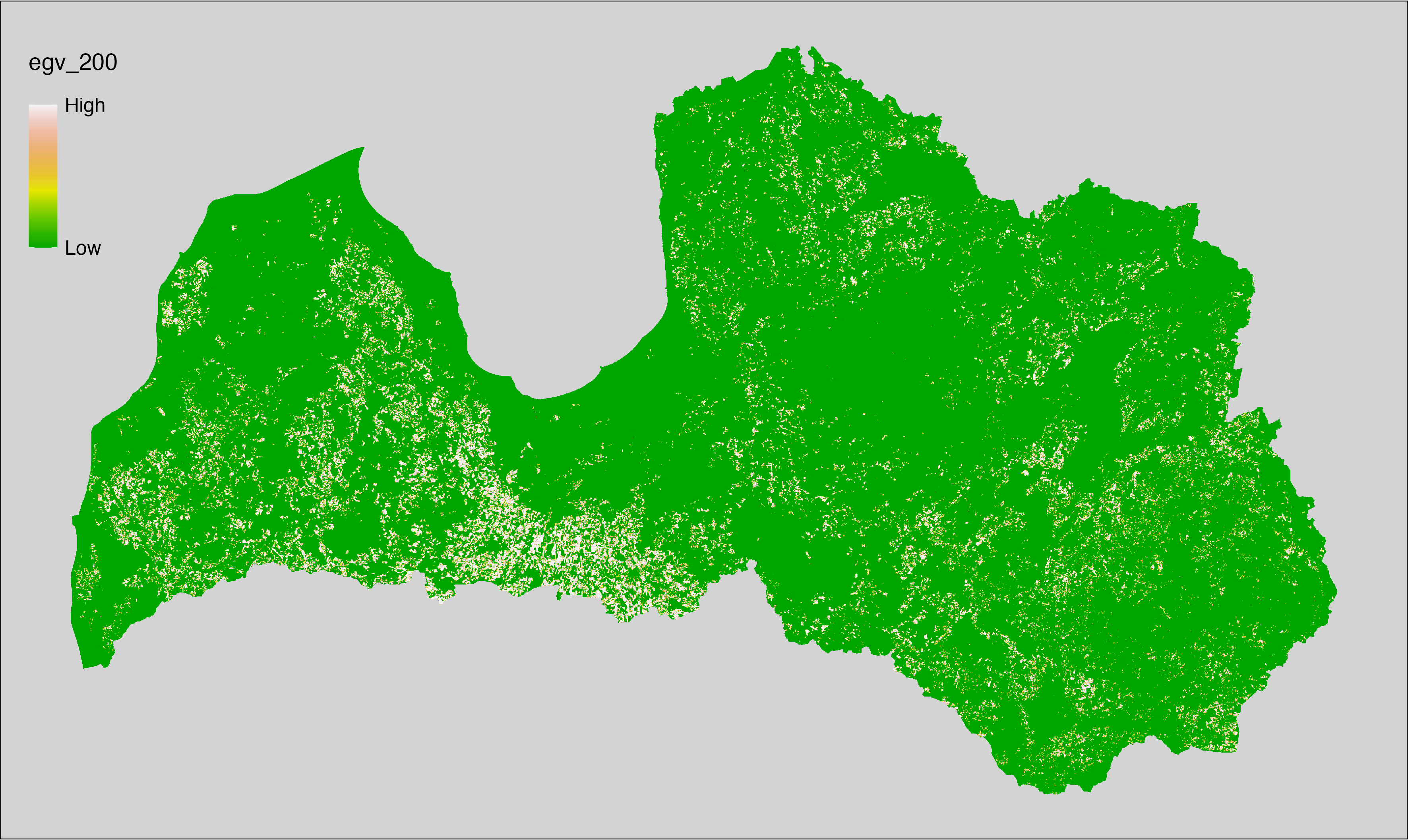
6.201 FarmlandCrops_CropsWinter_r500
filename: FarmlandCrops_CropsWinter_r500.tif
layername: egv_201
English name: Fractional cover of Winter Crops within the 0.5 km landscape
Latvian name: Ziemāju aramzemēs platības īpatsvars 0,5 km ainavā
Procedure: The cover fraction within a radius of 500 m around the analysis grid cell is
calculated as the area-weighted sum of the analysis cells inside the
buffer, using the workflow egvtools::radius_function(). During the calculation of the landscape metric,
inverse distance weighted (power = 2) gap filling on the output is applied
to ensure no missing values at the edges. Then the layer is rewritten to set
its name. Finally, the layer is standardised by subtracting the arithmetic
mean and dividing by the root mean squared error.
Code
# libs ----
if(!require(terra)) {install.packages("terra"); require(terra)}
if(!require(egvtools)) {remotes::install_github("aavotins/egvtools"); require(egvtools)}
# Templates -----
template100=rast("./Templates/TemplateRasters/LV100m_10km.tif")
# radii ----
radius_function(
kvadrati_path = "./Templates/TemplateGrids/tiles/",
radii_path = "./Templates/TemplateGridPoints/tiles/",
tikls100_path = "./Templates/TemplateGrids/tikls100_sauzeme.parquet",
template_path = "./Templates/TemplateRasters/LV100m_10km.tif",
input_layers = c("./RasterGrids_100m/2024/RAW/FarmlandCrops_CropsWinter_cell.tif"),
layer_prefixes = c("FarmlandCrops_CropsWinter"),
output_dir = "./RasterGrids_100m/2024/RAW/",
n_workers = 6,
radii = c("r500"),
radius_mode = "sparse",
extract_fun = "mean",
fill_missing = TRUE,
IDW_weight = 2,
future_max_size = 40 * 1024^3)
# FarmlandCrops_CropsWinter_r500.tif egv_201 ----
slanis=rast("./RasterGrids_100m/2024/RAW/FarmlandCrops_CropsWinter_r500.tif")
names(slanis)="egv_201"
slanis2=project(slanis,template100)
writeRaster(slanis2,
"./RasterGrids_100m/2024/RAW/FarmlandCrops_CropsWinter_r500.tif",
overwrite=TRUE)
# standardisation ----
if(!require(terra)) {install.packages("terra"); require(terra)}
if(!require(tidyverse)) {install.packages("tidyverse"); require(tidyverse)}
nosaukums="FarmlandCrops_CropsWinter_r500.tif"
ielasisanas_cels=paste0("./RasterGrids_100m/2024/RAW/",nosaukums)
saglabasanas_cels=paste0("./RasterGrids_100m/2024/Scaled/",nosaukums)
slanis=rast(ielasisanas_cels)
videjais=global(slanis,fun="mean",na.rm=TRUE)
centrets=slanis-videjais[,1]
standartnovirze=terra::global(centrets,fun="rms",na.rm=TRUE)
merogots=centrets/standartnovirze[,1]
writeRaster(merogots,
filename=saglabasanas_cels,
overwrite=TRUE)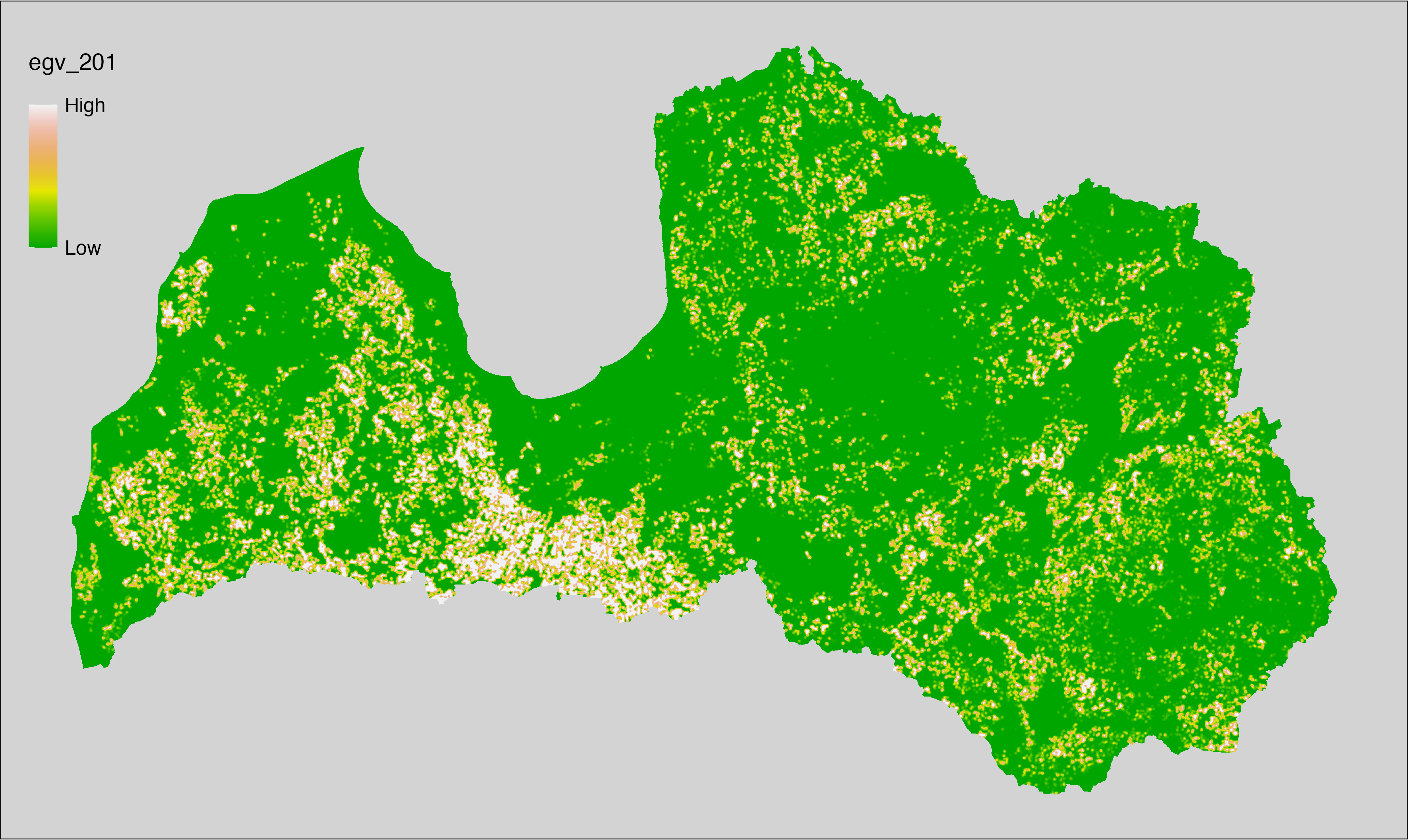
6.202 FarmlandCrops_CropsWinter_r1250
filename: FarmlandCrops_CropsWinter_r1250.tif
layername: egv_202
English name: Fractional cover of Winter Crops within the 1.25 km landscape
Latvian name: Ziemāju aramzemēs platības īpatsvars 1,25 km ainavā
Procedure: The cover fraction within a radius of 1250 m around the analysis grid cell
is calculated as the area-weighted sum of the analysis cells inside
the buffer, using the workflow egvtools::radius_function(). During the calculation of the landscape
metric, inverse distance weighted (power = 2) gap filling on the output is
applied to ensure no missing values at the edges. Then the layer is
rewritten to set its name. Finally, the layer is standardised by
subtracting the arithmetic mean and dividing by the root mean squared error.
Code
# libs ----
if(!require(terra)) {install.packages("terra"); require(terra)}
if(!require(egvtools)) {remotes::install_github("aavotins/egvtools"); require(egvtools)}
# Templates -----
template100=rast("./Templates/TemplateRasters/LV100m_10km.tif")
# radii ----
radius_function(
kvadrati_path = "./Templates/TemplateGrids/tiles/",
radii_path = "./Templates/TemplateGridPoints/tiles/",
tikls100_path = "./Templates/TemplateGrids/tikls100_sauzeme.parquet",
template_path = "./Templates/TemplateRasters/LV100m_10km.tif",
input_layers = c("./RasterGrids_100m/2024/RAW/FarmlandCrops_CropsWinter_cell.tif"),
layer_prefixes = c("FarmlandCrops_CropsWinter"),
output_dir = "./RasterGrids_100m/2024/RAW/",
n_workers = 6,
radii = c("r1250"),
radius_mode = "sparse",
extract_fun = "mean",
fill_missing = TRUE,
IDW_weight = 2,
future_max_size = 40 * 1024^3)
# FarmlandCrops_CropsWinter_r1250.tif egv_202 ----
slanis=rast("./RasterGrids_100m/2024/RAW/FarmlandCrops_CropsWinter_r1250.tif")
names(slanis)="egv_202"
slanis2=project(slanis,template100)
writeRaster(slanis2,
"./RasterGrids_100m/2024/RAW/FarmlandCrops_CropsWinter_r1250.tif",
overwrite=TRUE)
# standardisation ----
if(!require(terra)) {install.packages("terra"); require(terra)}
if(!require(tidyverse)) {install.packages("tidyverse"); require(tidyverse)}
nosaukums="FarmlandCrops_CropsWinter_r1250.tif"
ielasisanas_cels=paste0("./RasterGrids_100m/2024/RAW/",nosaukums)
saglabasanas_cels=paste0("./RasterGrids_100m/2024/Scaled/",nosaukums)
slanis=rast(ielasisanas_cels)
videjais=global(slanis,fun="mean",na.rm=TRUE)
centrets=slanis-videjais[,1]
standartnovirze=terra::global(centrets,fun="rms",na.rm=TRUE)
merogots=centrets/standartnovirze[,1]
writeRaster(merogots,
filename=saglabasanas_cels,
overwrite=TRUE)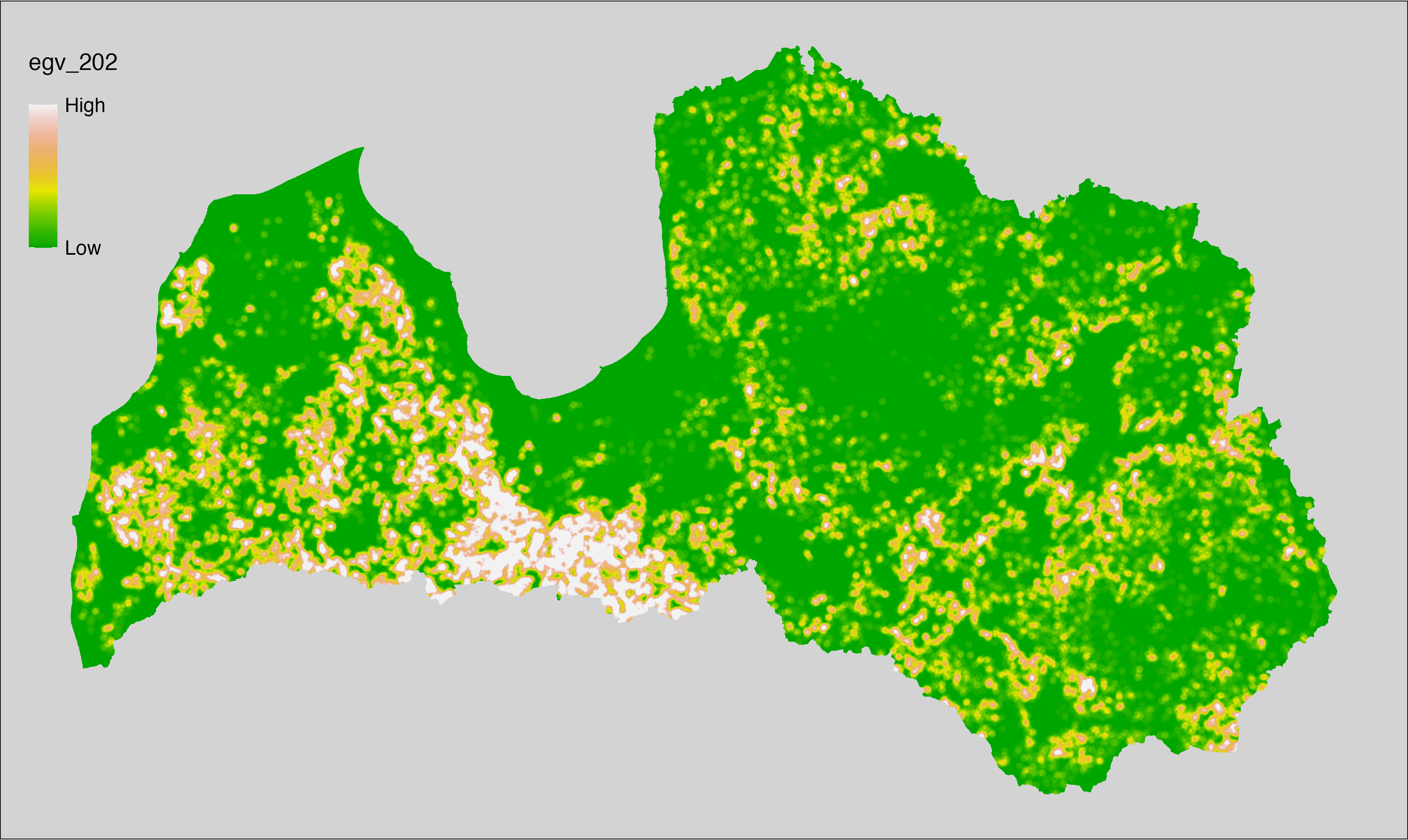
6.203 FarmlandCrops_CropsWinter_r3000
filename: FarmlandCrops_CropsWinter_r3000.tif
layername: egv_203
English name: Fractional cover of Winter Crops within the 3 km landscape
Latvian name: Ziemāju aramzemēs platības īpatsvars 3 km ainavā
Procedure: The cover fraction within a radius of 3000 m around the analysis grid cell
is calculated as the area-weighted sum of the analysis cells inside
the buffer, using the workflow egvtools::radius_function(). During the calculation of the landscape
metric, inverse distance weighted (power = 2) gap filling on the output is
applied to ensure no missing values at the edges. Then the layer is
rewritten to set its name. Finally, the layer is standardised by
subtracting the arithmetic mean and dividing by the root mean squared error.
Code
# libs ----
if(!require(terra)) {install.packages("terra"); require(terra)}
if(!require(egvtools)) {remotes::install_github("aavotins/egvtools"); require(egvtools)}
# Templates -----
template100=rast("./Templates/TemplateRasters/LV100m_10km.tif")
# radii ----
radius_function(
kvadrati_path = "./Templates/TemplateGrids/tiles/",
radii_path = "./Templates/TemplateGridPoints/tiles/",
tikls100_path = "./Templates/TemplateGrids/tikls100_sauzeme.parquet",
template_path = "./Templates/TemplateRasters/LV100m_10km.tif",
input_layers = c("./RasterGrids_100m/2024/RAW/FarmlandCrops_CropsWinter_cell.tif"),
layer_prefixes = c("FarmlandCrops_CropsWinter"),
output_dir = "./RasterGrids_100m/2024/RAW/",
n_workers = 6,
radii = c("r3000"),
radius_mode = "sparse",
extract_fun = "mean",
fill_missing = TRUE,
IDW_weight = 2,
future_max_size = 40 * 1024^3)
# FarmlandCrops_CropsWinter_r3000.tif egv_203 ----
slanis=rast("./RasterGrids_100m/2024/RAW/FarmlandCrops_CropsWinter_r3000.tif")
names(slanis)="egv_203"
slanis2=project(slanis,template100)
writeRaster(slanis2,
"./RasterGrids_100m/2024/RAW/FarmlandCrops_CropsWinter_r3000.tif",
overwrite=TRUE)
# standardisation ----
if(!require(terra)) {install.packages("terra"); require(terra)}
if(!require(tidyverse)) {install.packages("tidyverse"); require(tidyverse)}
nosaukums="FarmlandCrops_CropsWinter_r3000.tif"
ielasisanas_cels=paste0("./RasterGrids_100m/2024/RAW/",nosaukums)
saglabasanas_cels=paste0("./RasterGrids_100m/2024/Scaled/",nosaukums)
slanis=rast(ielasisanas_cels)
videjais=global(slanis,fun="mean",na.rm=TRUE)
centrets=slanis-videjais[,1]
standartnovirze=terra::global(centrets,fun="rms",na.rm=TRUE)
merogots=centrets/standartnovirze[,1]
writeRaster(merogots,
filename=saglabasanas_cels,
overwrite=TRUE)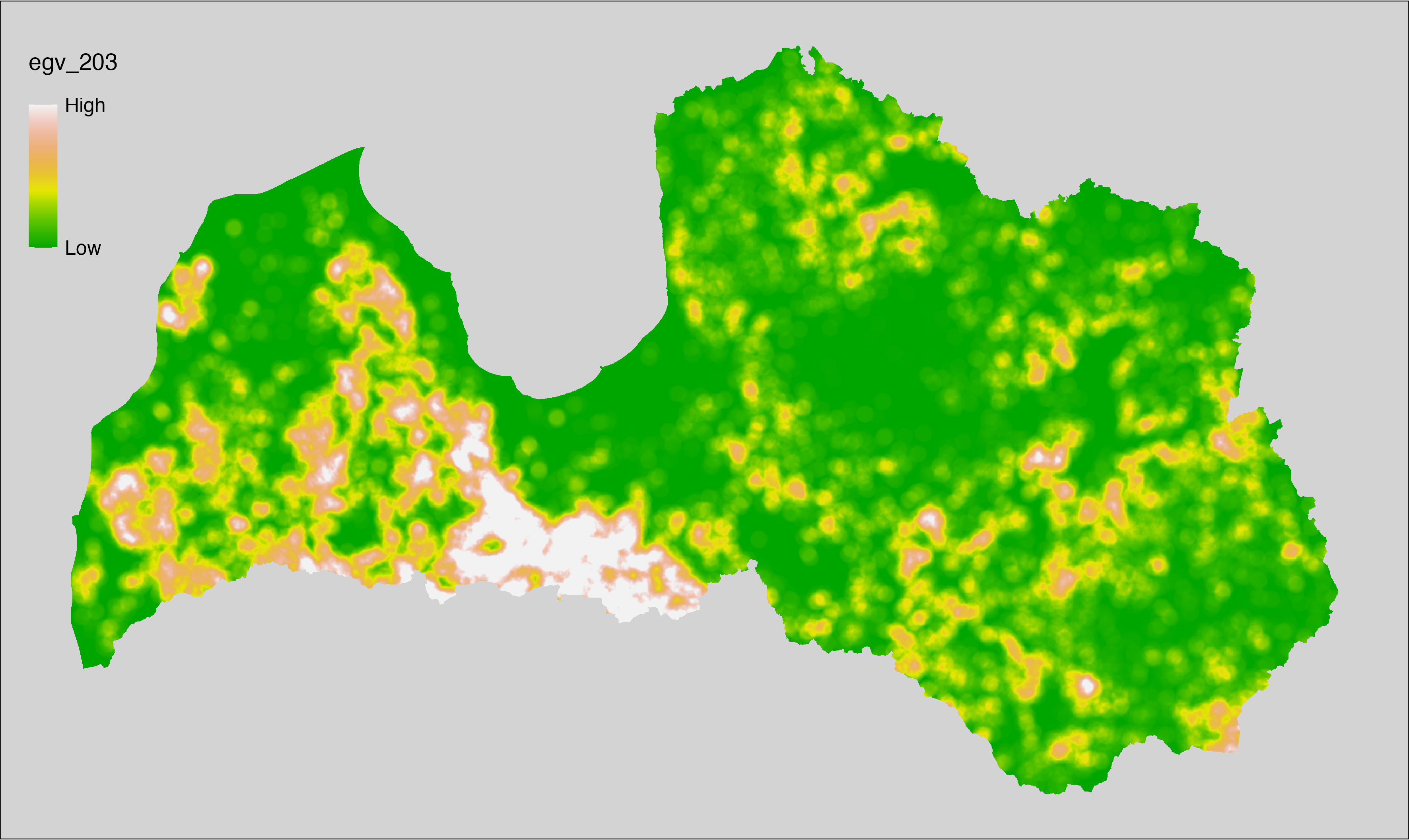
6.204 FarmlandCrops_CropsWinter_r10000
filename: FarmlandCrops_CropsWinter_r10000.tif
layername: egv_204
English name: Fractional cover of Winter Crops within the 10 km landscape
Latvian name: Ziemāju aramzemēs platības īpatsvars 10 km ainavā
Procedure: The cover fraction within a radius of 10000 m around the analysis grid cell
is calculated as the area-weighted sum of the analysis cells inside
the buffer, using the workflow egvtools::radius_function(). During the calculation of the landscape
metric, inverse distance weighted (power = 2) gap filling on the output is
applied to ensure no missing values at the edges. Then the layer is
rewritten to set its name. Finally, the layer is standardised by
subtracting the arithmetic mean and dividing by the root mean squared error.
Code
# libs ----
if(!require(terra)) {install.packages("terra"); require(terra)}
if(!require(egvtools)) {remotes::install_github("aavotins/egvtools"); require(egvtools)}
# Templates -----
template100=rast("./Templates/TemplateRasters/LV100m_10km.tif")
# radii ----
radius_function(
kvadrati_path = "./Templates/TemplateGrids/tiles/",
radii_path = "./Templates/TemplateGridPoints/tiles/",
tikls100_path = "./Templates/TemplateGrids/tikls100_sauzeme.parquet",
template_path = "./Templates/TemplateRasters/LV100m_10km.tif",
input_layers = c("./RasterGrids_100m/2024/RAW/FarmlandCrops_CropsWinter_cell.tif"),
layer_prefixes = c("FarmlandCrops_CropsWinter"),
output_dir = "./RasterGrids_100m/2024/RAW/",
n_workers = 6,
radii = c("r10000"),
radius_mode = "sparse",
extract_fun = "mean",
fill_missing = TRUE,
IDW_weight = 2,
future_max_size = 40 * 1024^3)
# FarmlandCrops_CropsWinter_r10000.tif egv_204 ----
slanis=rast("./RasterGrids_100m/2024/RAW/FarmlandCrops_CropsWinter_r10000.tif")
names(slanis)="egv_204"
slanis2=project(slanis,template100)
writeRaster(slanis2,
"./RasterGrids_100m/2024/RAW/FarmlandCrops_CropsWinter_r10000.tif",
overwrite=TRUE)
# standardisation ----
if(!require(terra)) {install.packages("terra"); require(terra)}
if(!require(tidyverse)) {install.packages("tidyverse"); require(tidyverse)}
nosaukums="FarmlandCrops_CropsWinter_r10000.tif"
ielasisanas_cels=paste0("./RasterGrids_100m/2024/RAW/",nosaukums)
saglabasanas_cels=paste0("./RasterGrids_100m/2024/Scaled/",nosaukums)
slanis=rast(ielasisanas_cels)
videjais=global(slanis,fun="mean",na.rm=TRUE)
centrets=slanis-videjais[,1]
standartnovirze=terra::global(centrets,fun="rms",na.rm=TRUE)
merogots=centrets/standartnovirze[,1]
writeRaster(merogots,
filename=saglabasanas_cels,
overwrite=TRUE)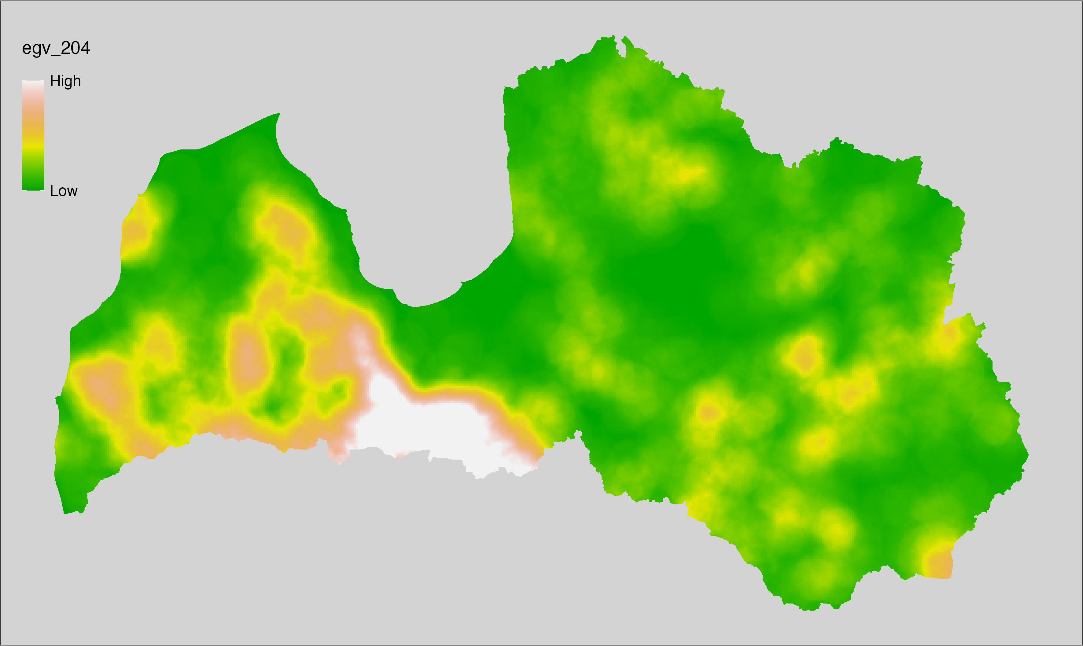
6.205 FarmlandCrops_RapeseedsSpring_cell
filename: FarmlandCrops_RapeseedsSpring_cell.tif
layername: egv_205
English name: Fractional cover of Spring Sown Rapeseed, Turnip, Corn within the analysis cell (1 ha)
Latvian name: Vasaras rapša, ripša, kukurūzas platība analīzes šūnā (1 ha)
Procedure: First, agricultural parcels declared as spring sown
rapeseed, turnip or corn are selected from the Rural Support Service’s information
on declared fields. These geometries are then rasterised to input
resolution, ensuring value 1 at the polygon locations and value 0 elsewhere.
Rasterisation is performed using the workflow egvtools::polygon2input(). Once
rasterised, the layer is aggregated to EGV
resolution using the workflow egvtools::input2egv(), which calculates the arithmetic mean and thus
results in a cover fraction. During aggregation, inverse
distance weighted (power = 2) gap filling on the output is applied to
ensure no missing values at the edges. Finally, the layer is standardised
by subtracting the arithmetic mean and dividing by the root mean squared error.
Code
# libs ----
if(!require(egvtools)) {remotes::install_github("aavotins/egvtools"); require(egvtools)}
if(!require(terra)) {install.packages("terra"); require(terra)}
if(!require(sf)) {install.packages("sf"); require(sf)}
if(!require(tidyverse)) {install.packages("tidyverse"); require(tidyverse)}
if(!require(sfarrow)) {install.packages("sfarrow"); require(sfarrow)}
if(!require(readxl)) {install.packages("readxl"); require(readxl)}
if(!require(raster)) {install.packages("raster"); require(raster)}
if(!require(fasterize)) {install.packages("fasterize"); require(fasterize)}
# templates ----
template100=rast("./Templates/TemplateRasters/LV100m_10km.tif")
template10=rast("./Templates/TemplateRasters/LV10m_10km.tif")
rastrs10=raster(template10)
nulls10=rast("./Templates/TemplateRasters/nulls_LV10m_10km.tif")
nulls100=rast("./Templates/TemplateRasters/nulls_LV100m_10km.tif")
# codes ----
kodi=read_excel("./Geodata/2024/LAD/KulturuKodi_2024.xlsx")
kodi$kods=as.character(kodi$kods)
# LAD ----
lad=sfarrow::st_read_parquet("./Geodata/2024/LAD/Lauki_2024.parquet")
lad$yes=1
lad=lad %>%
left_join(kodi,by=c("PRODUCT_CODE"="kods"))
# simple landscape ----
simple_landscape=rast("RasterGrids_10m/2024/Ainava_vienk_mask.tif")
# FarmlandCrops_RapeseedsSpring_cell.tif egv_205 ----
dati=lad %>%
filter(str_detect(SDM_grupa_sakums,"vasaras rapsis"))
table(dati$SDM_grupa_sakums,useNA="always")
p2i_rez=egvtools::polygon2input(vector_data = dati,
template_path = "./Templates/TemplateRasters/LV10m_10km.tif",
out_path = "./RasterGrids_10m/2024/",
file_name = "FarmlandCrops_RapeseedsSpring_input.tif",
value_field = "yes",
prepare=FALSE,
background_raster = "./Templates/TemplateRasters/nulls_LV10m_10km.tif",
plot_result = TRUE)
p2i_rez
i2e_rez=egvtools::input2egv(input=paste0("./RasterGrids_10m/2024/",
"FarmlandCrops_RapeseedsSpring_input.tif"),
egv_template= "./Templates/TemplateRasters/LV100m_10km.tif",
summary_function = "average",
missing_job = "FillOutput",
outlocation = "./RasterGrids_100m/2024/RAW/",
outfilename = "FarmlandCrops_RapeseedsSpring_cell.tif",
layername = "egv_205",
idw_weight = 2,
plot_gaps = FALSE,plot_final = TRUE)
i2e_rez
rm(p2i_rez)
rm(i2e_rez)
rm(dati)
unlink("./RasterGrids_10m/2024/FarmlandCrops_RapeseedsSpring_input.tif")
# standardisation ----
if(!require(terra)) {install.packages("terra"); require(terra)}
if(!require(tidyverse)) {install.packages("tidyverse"); require(tidyverse)}
nosaukums="FarmlandCrops_RapeseedsSpring_cell.tif"
ielasisanas_cels=paste0("./RasterGrids_100m/2024/RAW/",nosaukums)
saglabasanas_cels=paste0("./RasterGrids_100m/2024/Scaled/",nosaukums)
slanis=rast(ielasisanas_cels)
videjais=global(slanis,fun="mean",na.rm=TRUE)
centrets=slanis-videjais[,1]
standartnovirze=terra::global(centrets,fun="rms",na.rm=TRUE)
merogots=centrets/standartnovirze[,1]
writeRaster(merogots,
filename=saglabasanas_cels,
overwrite=TRUE)
6.206 FarmlandCrops_RapeseedsSpring_r500
filename: FarmlandCrops_RapeseedsSpring_r500.tif
layername: egv_206
English name: Fractional cover of Spring Sown Rapeseed, Turnip, Corn within the 0.5 km landscape
Latvian name: Vasaras rapša, ripša, kukurūzas platība 0,5 km ainavā
Procedure: The cover fraction within a radius of 500 m around the analysis grid cell is
calculated as the area-weighted sum of the analysis cells inside the
buffer, using the workflow egvtools::radius_function(). During the calculation of the landscape metric,
inverse distance weighted (power = 2) gap filling on the output is applied
to ensure no missing values at the edges. Then the layer is rewritten to set
its name. Finally, the layer is standardised by subtracting the arithmetic
mean and dividing by the root mean squared error.
Code
# libs ----
if(!require(terra)) {install.packages("terra"); require(terra)}
if(!require(egvtools)) {remotes::install_github("aavotins/egvtools"); require(egvtools)}
# Templates -----
template100=rast("./Templates/TemplateRasters/LV100m_10km.tif")
# radii ----
radius_function(
kvadrati_path = "./Templates/TemplateGrids/tiles/",
radii_path = "./Templates/TemplateGridPoints/tiles/",
tikls100_path = "./Templates/TemplateGrids/tikls100_sauzeme.parquet",
template_path = "./Templates/TemplateRasters/LV100m_10km.tif",
input_layers = c("./RasterGrids_100m/2024/RAW/FarmlandCrops_RapeseedsSpring_cell.tif"),
layer_prefixes = c("FarmlandCrops_RapeseedsSpring"),
output_dir = "./RasterGrids_100m/2024/RAW/",
n_workers = 6,
radii = c("r500"),
radius_mode = "sparse",
extract_fun = "mean",
fill_missing = TRUE,
IDW_weight = 2,
future_max_size = 40 * 1024^3)
# FarmlandCrops_RapeseedsSpring_r500.tif egv_206
slanis=rast("./RasterGrids_100m/2024/RAW/FarmlandCrops_RapeseedsSpring_r500.tif")
names(slanis)="egv_206"
slanis2=project(slanis,template100)
writeRaster(slanis2,
"./RasterGrids_100m/2024/RAW/FarmlandCrops_RapeseedsSpring_r500.tif",
overwrite=TRUE)
# standardisation ----
if(!require(terra)) {install.packages("terra"); require(terra)}
if(!require(tidyverse)) {install.packages("tidyverse"); require(tidyverse)}
nosaukums="FarmlandCrops_RapeseedsSpring_r500.tif"
ielasisanas_cels=paste0("./RasterGrids_100m/2024/RAW/",nosaukums)
saglabasanas_cels=paste0("./RasterGrids_100m/2024/Scaled/",nosaukums)
slanis=rast(ielasisanas_cels)
videjais=global(slanis,fun="mean",na.rm=TRUE)
centrets=slanis-videjais[,1]
standartnovirze=terra::global(centrets,fun="rms",na.rm=TRUE)
merogots=centrets/standartnovirze[,1]
writeRaster(merogots,
filename=saglabasanas_cels,
overwrite=TRUE)
6.207 FarmlandCrops_RapeseedsSpring_r1250
filename: FarmlandCrops_RapeseedsSpring_r1250.tif
layername: egv_207
English name: Fractional cover of Spring Sown Rapeseed, Turnip, Corn within the 1.25 km landscape
Latvian name: Vasaras rapša, ripša, kukurūzas platība 1,25 km ainavā
Procedure: The cover fraction within a radius of 1250 m around the analysis grid cell
is calculated as the area-weighted sum of the analysis cells inside
the buffer, using the workflow egvtools::radius_function(). During the calculation of the landscape
metric, inverse distance weighted (power = 2) gap filling on the output is
applied to ensure no missing values at the edges. Then the layer is
rewritten to set its name. Finally, the layer is standardised by
subtracting the arithmetic mean and dividing by the root mean squared error.
Code
# libs ----
if(!require(terra)) {install.packages("terra"); require(terra)}
if(!require(egvtools)) {remotes::install_github("aavotins/egvtools"); require(egvtools)}
# Templates -----
template100=rast("./Templates/TemplateRasters/LV100m_10km.tif")
# radii ----
radius_function(
kvadrati_path = "./Templates/TemplateGrids/tiles/",
radii_path = "./Templates/TemplateGridPoints/tiles/",
tikls100_path = "./Templates/TemplateGrids/tikls100_sauzeme.parquet",
template_path = "./Templates/TemplateRasters/LV100m_10km.tif",
input_layers = c("./RasterGrids_100m/2024/RAW/FarmlandCrops_RapeseedsSpring_cell.tif"),
layer_prefixes = c("FarmlandCrops_RapeseedsSpring"),
output_dir = "./RasterGrids_100m/2024/RAW/",
n_workers = 6,
radii = c("r1250"),
radius_mode = "sparse",
extract_fun = "mean",
fill_missing = TRUE,
IDW_weight = 2,
future_max_size = 40 * 1024^3)
# FarmlandCrops_RapeseedsSpring_r1250.tif egv_207
slanis=rast("./RasterGrids_100m/2024/RAW/FarmlandCrops_RapeseedsSpring_r1250.tif")
names(slanis)="egv_207"
slanis2=project(slanis,template100)
writeRaster(slanis2,
"./RasterGrids_100m/2024/RAW/FarmlandCrops_RapeseedsSpring_r1250.tif",
overwrite=TRUE)
# standardisation ----
if(!require(terra)) {install.packages("terra"); require(terra)}
if(!require(tidyverse)) {install.packages("tidyverse"); require(tidyverse)}
nosaukums="FarmlandCrops_RapeseedsSpring_r1250.tif"
ielasisanas_cels=paste0("./RasterGrids_100m/2024/RAW/",nosaukums)
saglabasanas_cels=paste0("./RasterGrids_100m/2024/Scaled/",nosaukums)
slanis=rast(ielasisanas_cels)
videjais=global(slanis,fun="mean",na.rm=TRUE)
centrets=slanis-videjais[,1]
standartnovirze=terra::global(centrets,fun="rms",na.rm=TRUE)
merogots=centrets/standartnovirze[,1]
writeRaster(merogots,
filename=saglabasanas_cels,
overwrite=TRUE)
6.208 FarmlandCrops_RapeseedsSpring_r3000
filename: FarmlandCrops_RapeseedsSpring_r3000.tif
layername: egv_208
English name: Fractional cover of Spring Sown Rapeseed, Turnip, Corn within the 3 km landscape
Latvian name: Vasaras rapša, ripša, kukurūzas platība 3 km ainavā
Procedure: The cover fraction within a radius of 3000 m around the analysis grid cell
is calculated as the area-weighted sum of the analysis cells inside
the buffer, using the workflow egvtools::radius_function(). During the calculation of the landscape
metric, inverse distance weighted (power = 2) gap filling on the output is
applied to ensure no missing values at the edges. Then the layer is
rewritten to set its name. Finally, the layer is standardised by
subtracting the arithmetic mean and dividing by the root mean squared error.
Code
# libs ----
if(!require(terra)) {install.packages("terra"); require(terra)}
if(!require(egvtools)) {remotes::install_github("aavotins/egvtools"); require(egvtools)}
# Templates -----
template100=rast("./Templates/TemplateRasters/LV100m_10km.tif")
# radii ----
radius_function(
kvadrati_path = "./Templates/TemplateGrids/tiles/",
radii_path = "./Templates/TemplateGridPoints/tiles/",
tikls100_path = "./Templates/TemplateGrids/tikls100_sauzeme.parquet",
template_path = "./Templates/TemplateRasters/LV100m_10km.tif",
input_layers = c("./RasterGrids_100m/2024/RAW/FarmlandCrops_RapeseedsSpring_cell.tif"),
layer_prefixes = c("FarmlandCrops_RapeseedsSpring"),
output_dir = "./RasterGrids_100m/2024/RAW/",
n_workers = 6,
radii = c("r3000"),
radius_mode = "sparse",
extract_fun = "mean",
fill_missing = TRUE,
IDW_weight = 2,
future_max_size = 40 * 1024^3)
# FarmlandCrops_RapeseedsSpring_r3000.tif egv_208
slanis=rast("./RasterGrids_100m/2024/RAW/FarmlandCrops_RapeseedsSpring_r3000.tif")
names(slanis)="egv_208"
slanis2=project(slanis,template100)
writeRaster(slanis2,
"./RasterGrids_100m/2024/RAW/FarmlandCrops_RapeseedsSpring_r3000.tif",
overwrite=TRUE)
# standardisation ----
if(!require(terra)) {install.packages("terra"); require(terra)}
if(!require(tidyverse)) {install.packages("tidyverse"); require(tidyverse)}
nosaukums="FarmlandCrops_RapeseedsSpring_r3000.tif"
ielasisanas_cels=paste0("./RasterGrids_100m/2024/RAW/",nosaukums)
saglabasanas_cels=paste0("./RasterGrids_100m/2024/Scaled/",nosaukums)
slanis=rast(ielasisanas_cels)
videjais=global(slanis,fun="mean",na.rm=TRUE)
centrets=slanis-videjais[,1]
standartnovirze=terra::global(centrets,fun="rms",na.rm=TRUE)
merogots=centrets/standartnovirze[,1]
writeRaster(merogots,
filename=saglabasanas_cels,
overwrite=TRUE)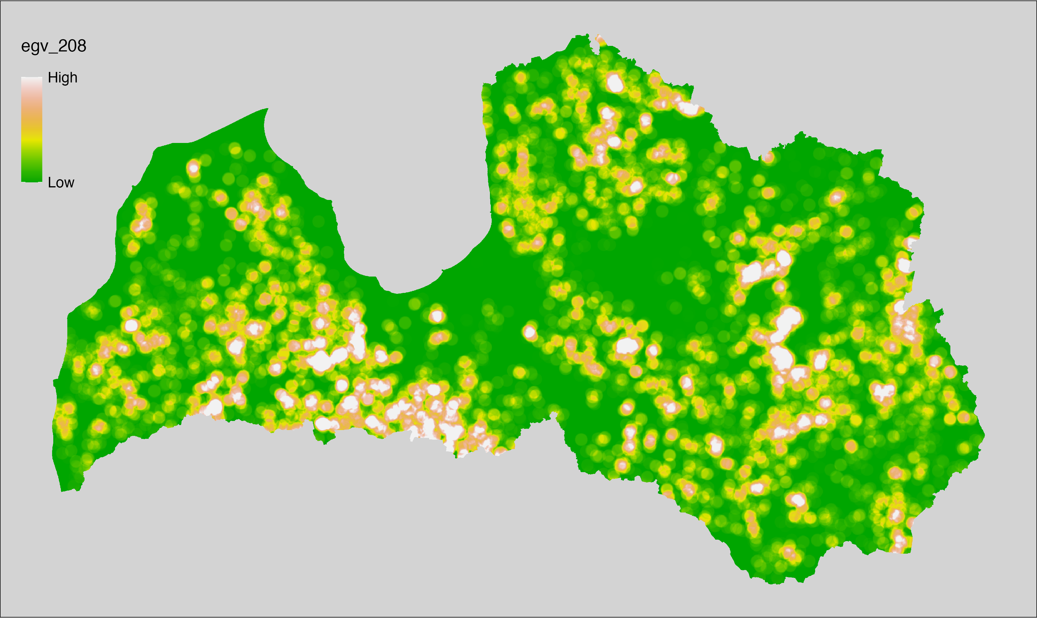
6.209 FarmlandCrops_RapeseedsSpring_r10000
filename: FarmlandCrops_RapeseedsSpring_r10000.tif
layername: egv_209
English name: Fractional cover of Spring Sown Rapeseed, Turnip, Corn within the 10 km landscape
Latvian name: Vasaras rapša, ripša, kukurūzas platība 10 km ainavā
Procedure: The cover fraction within a radius of 10000 m around the analysis grid cell
is calculated as the area-weighted sum of the analysis cells inside
the buffer, using the workflow egvtools::radius_function(). During the calculation of the landscape
metric, inverse distance weighted (power = 2) gap filling on the output is
applied to ensure no missing values at the edges. Then the layer is
rewritten to set its name. Finally, the layer is standardised by
subtracting the arithmetic mean and dividing by the root mean squared error.
Code
# libs ----
if(!require(terra)) {install.packages("terra"); require(terra)}
if(!require(egvtools)) {remotes::install_github("aavotins/egvtools"); require(egvtools)}
# Templates -----
template100=rast("./Templates/TemplateRasters/LV100m_10km.tif")
# radii ----
radius_function(
kvadrati_path = "./Templates/TemplateGrids/tiles/",
radii_path = "./Templates/TemplateGridPoints/tiles/",
tikls100_path = "./Templates/TemplateGrids/tikls100_sauzeme.parquet",
template_path = "./Templates/TemplateRasters/LV100m_10km.tif",
input_layers = c("./RasterGrids_100m/2024/RAW/FarmlandCrops_RapeseedsSpring_cell.tif"),
layer_prefixes = c("FarmlandCrops_RapeseedsSpring"),
output_dir = "./RasterGrids_100m/2024/RAW/",
n_workers = 6,
radii = c("r10000"),
radius_mode = "sparse",
extract_fun = "mean",
fill_missing = TRUE,
IDW_weight = 2,
future_max_size = 40 * 1024^3)
# FarmlandCrops_RapeseedsSpring_r10000.tif egv_209
slanis=rast("./RasterGrids_100m/2024/RAW/FarmlandCrops_RapeseedsSpring_r10000.tif")
names(slanis)="egv_209"
slanis2=project(slanis,template100)
writeRaster(slanis2,
"./RasterGrids_100m/2024/RAW/FarmlandCrops_RapeseedsSpring_r10000.tif",
overwrite=TRUE)
# standardisation ----
if(!require(terra)) {install.packages("terra"); require(terra)}
if(!require(tidyverse)) {install.packages("tidyverse"); require(tidyverse)}
nosaukums="FarmlandCrops_RapeseedsSpring_r10000.tif"
ielasisanas_cels=paste0("./RasterGrids_100m/2024/RAW/",nosaukums)
saglabasanas_cels=paste0("./RasterGrids_100m/2024/Scaled/",nosaukums)
slanis=rast(ielasisanas_cels)
videjais=global(slanis,fun="mean",na.rm=TRUE)
centrets=slanis-videjais[,1]
standartnovirze=terra::global(centrets,fun="rms",na.rm=TRUE)
merogots=centrets/standartnovirze[,1]
writeRaster(merogots,
filename=saglabasanas_cels,
overwrite=TRUE)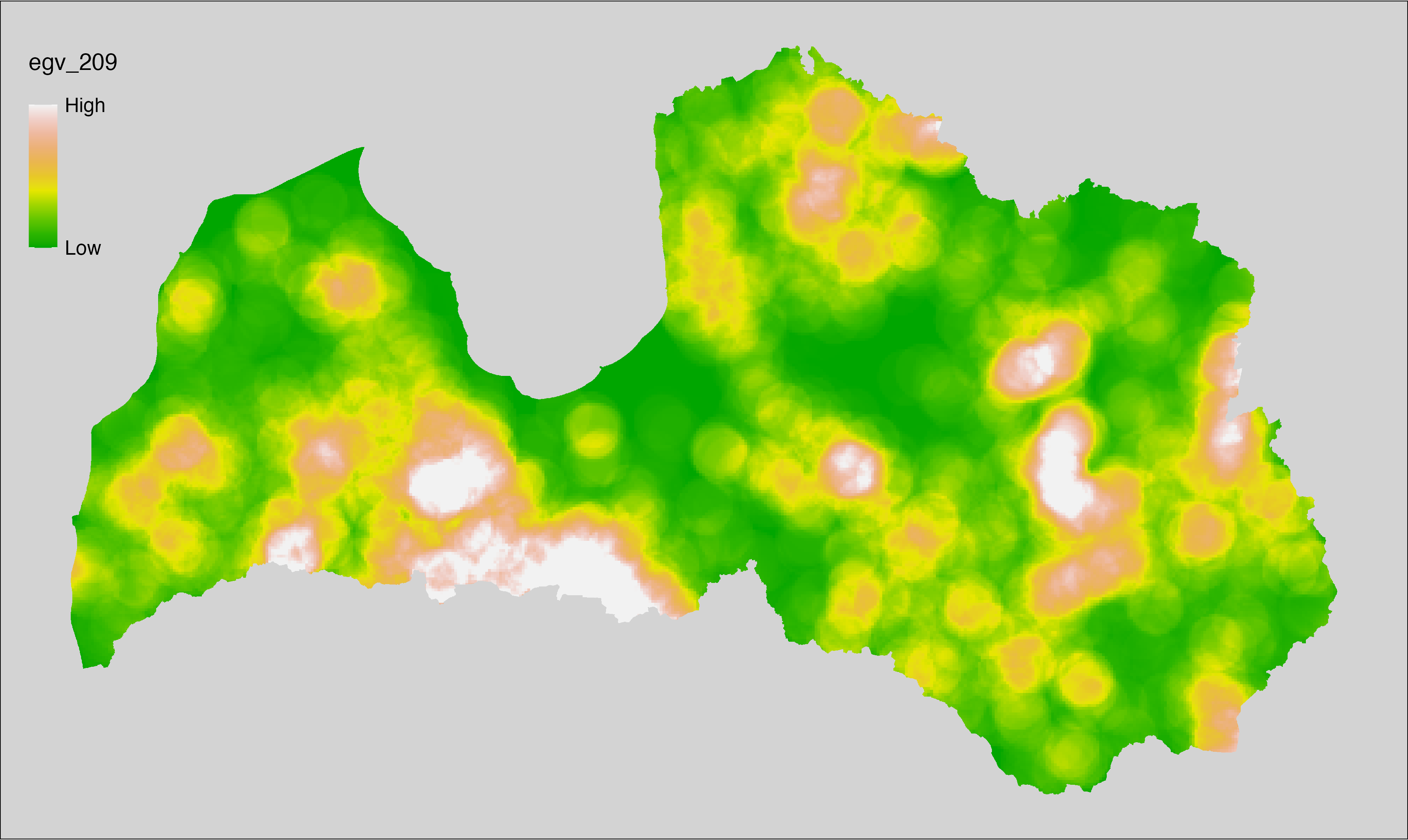
6.210 FarmlandCrops_RapeseedsWinter_cell
filename: FarmlandCrops_RapeseedsWinter_cell.tif
layername: egv_210
English name: Fractional cover of Winter Rapeseed, Turnip within the analysis cell (1 ha)
Latvian name: Ziemas rapša, ripša platības īpatsvars analīzes šūnā (1 ha)
Procedure: First, agricultural parcels declared as winter rapeseed or
turnip are selected from the Rural Support Service’s information on declared
fields. These geometries are then rasterised to input resolution,
ensuring value 1 at the polygon locations and value 0 elsewhere. Rasterisation is performed using the workflow egvtools::polygon2input(). Once rasterised, the layer is aggregated to EGV
resolution using the workflow egvtools::input2egv(), which calculates the arithmetic mean and thus
results in a cover fraction. During aggregation, inverse
distance weighted (power = 2) gap filling on the output is applied to
ensure no missing values at the edges. Finally, the layer is standardised
by subtracting the arithmetic mean and dividing by the root mean squared error.
Code
# libs ----
if(!require(egvtools)) {remotes::install_github("aavotins/egvtools"); require(egvtools)}
if(!require(terra)) {install.packages("terra"); require(terra)}
if(!require(sf)) {install.packages("sf"); require(sf)}
if(!require(tidyverse)) {install.packages("tidyverse"); require(tidyverse)}
if(!require(sfarrow)) {install.packages("sfarrow"); require(sfarrow)}
if(!require(readxl)) {install.packages("readxl"); require(readxl)}
if(!require(raster)) {install.packages("raster"); require(raster)}
if(!require(fasterize)) {install.packages("fasterize"); require(fasterize)}
# templates ----
template100=rast("./Templates/TemplateRasters/LV100m_10km.tif")
template10=rast("./Templates/TemplateRasters/LV10m_10km.tif")
rastrs10=raster(template10)
nulls10=rast("./Templates/TemplateRasters/nulls_LV10m_10km.tif")
nulls100=rast("./Templates/TemplateRasters/nulls_LV100m_10km.tif")
# codes ----
kodi=read_excel("./Geodata/2024/LAD/KulturuKodi_2024.xlsx")
kodi$kods=as.character(kodi$kods)
# LAD ----
lad=sfarrow::st_read_parquet("./Geodata/2024/LAD/Lauki_2024.parquet")
lad$yes=1
lad=lad %>%
left_join(kodi,by=c("PRODUCT_CODE"="kods"))
# simple landscape ----
simple_landscape=rast("RasterGrids_10m/2024/Ainava_vienk_mask.tif")
# FarmlandCrops_RapeseedsWinter_cell.tif egv_210 ----
dati=lad %>%
filter(str_detect(SDM_grupa_sakums,"ziemas rapsis"))
table(dati$SDM_grupa_sakums,useNA="always")
p2i_rez=egvtools::polygon2input(vector_data = dati,
template_path = "./Templates/TemplateRasters/LV10m_10km.tif",
out_path = "./RasterGrids_10m/2024/",
file_name = "FarmlandCrops_RapeseedsWinter_input.tif",
value_field = "yes",
prepare=FALSE,
background_raster = "./Templates/TemplateRasters/nulls_LV10m_10km.tif",
plot_result = TRUE)
p2i_rez
i2e_rez=egvtools::input2egv(input=paste0("./RasterGrids_10m/2024/",
"FarmlandCrops_RapeseedsWinter_input.tif"),
egv_template= "./Templates/TemplateRasters/LV100m_10km.tif",
summary_function = "average",
missing_job = "FillOutput",
outlocation = "./RasterGrids_100m/2024/RAW/",
outfilename = "FarmlandCrops_RapeseedsWinter_cell.tif",
layername = "egv_210",
idw_weight = 2,
plot_gaps = FALSE,plot_final = TRUE)
i2e_rez
rm(p2i_rez)
rm(i2e_rez)
rm(dati)
unlink("./RasterGrids_10m/2024/FarmlandCrops_RapeseedsWinter_input.tif")
# standardisation ----
if(!require(terra)) {install.packages("terra"); require(terra)}
if(!require(tidyverse)) {install.packages("tidyverse"); require(tidyverse)}
nosaukums="FarmlandCrops_RapeseedsWinter_cell.tif"
ielasisanas_cels=paste0("./RasterGrids_100m/2024/RAW/",nosaukums)
saglabasanas_cels=paste0("./RasterGrids_100m/2024/Scaled/",nosaukums)
slanis=rast(ielasisanas_cels)
videjais=global(slanis,fun="mean",na.rm=TRUE)
centrets=slanis-videjais[,1]
standartnovirze=terra::global(centrets,fun="rms",na.rm=TRUE)
merogots=centrets/standartnovirze[,1]
writeRaster(merogots,
filename=saglabasanas_cels,
overwrite=TRUE)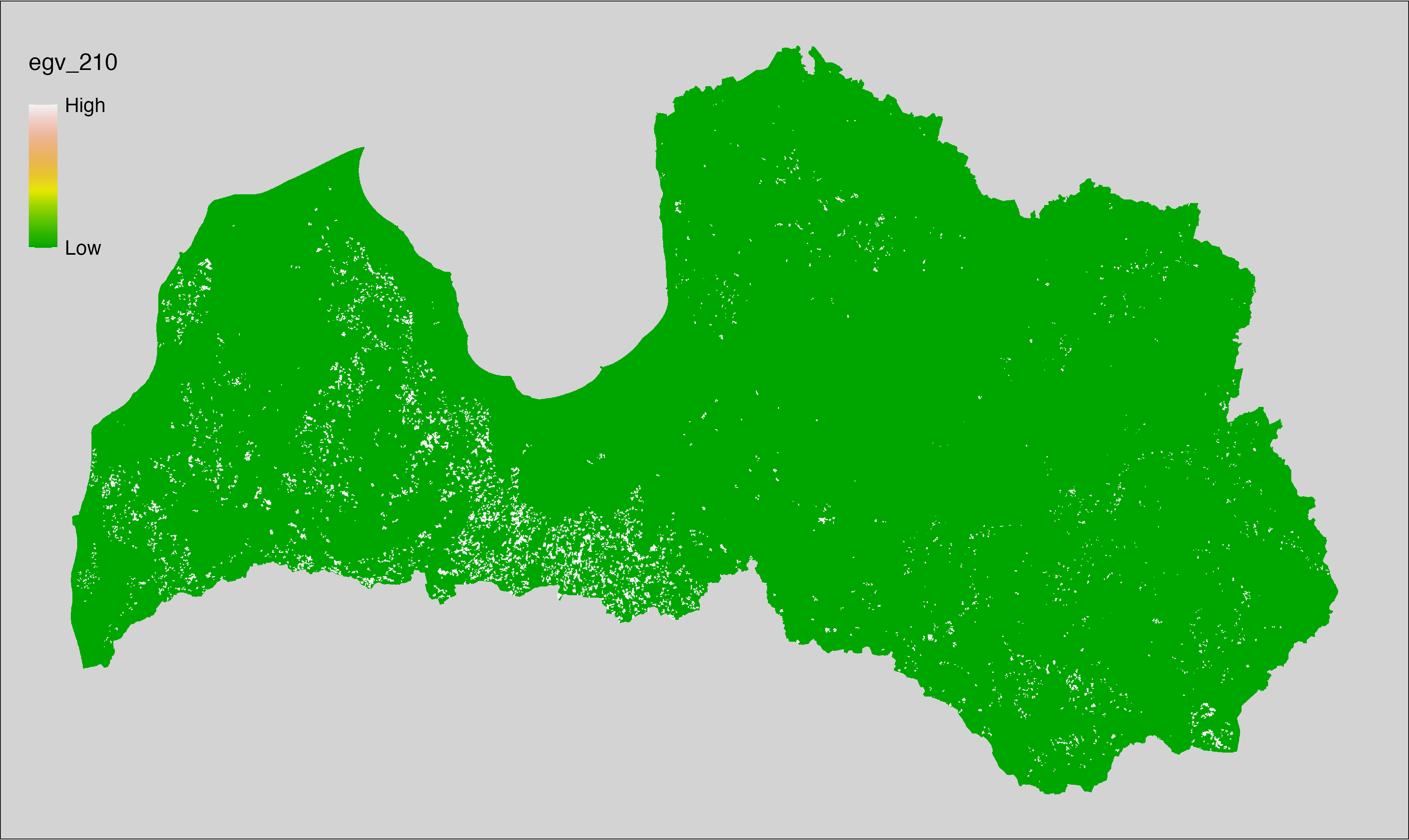
6.211 FarmlandCrops_RapeseedsWinter_r500
filename: FarmlandCrops_RapeseedsWinter_r500.tif
layername: egv_211
English name: Fractional cover of Winter Rapeseed, Turnip within the 0.5 km landscape
Latvian name: Ziemas rapša, ripša platības īpatsvars 0,5 km ainavā
Procedure: The cover fraction within a radius of 500 m around the analysis grid cell is
calculated as the area-weighted sum of the analysis cells inside the
buffer, using the workflow egvtools::radius_function(). During the calculation of the landscape metric,
inverse distance weighted (power = 2) gap filling on the output is applied
to ensure no missing values at the edges. Then the layer is rewritten to set
its name. Finally, the layer is standardised by subtracting the arithmetic
mean and dividing by the root mean squared error.
Code
# libs ----
if(!require(terra)) {install.packages("terra"); require(terra)}
if(!require(egvtools)) {remotes::install_github("aavotins/egvtools"); require(egvtools)}
# Templates -----
template100=rast("./Templates/TemplateRasters/LV100m_10km.tif")
# radii ----
radius_function(
kvadrati_path = "./Templates/TemplateGrids/tiles/",
radii_path = "./Templates/TemplateGridPoints/tiles/",
tikls100_path = "./Templates/TemplateGrids/tikls100_sauzeme.parquet",
template_path = "./Templates/TemplateRasters/LV100m_10km.tif",
input_layers = c("./RasterGrids_100m/2024/RAW/FarmlandCrops_RapeseedsWinter_cell.tif"),
layer_prefixes = c("FarmlandCrops_RapeseedsWinter"),
output_dir = "./RasterGrids_100m/2024/RAW/",
n_workers = 6,
radii = c("r500"),
radius_mode = "sparse",
extract_fun = "mean",
fill_missing = TRUE,
IDW_weight = 2,
future_max_size = 40 * 1024^3)
# FarmlandCrops_RapeseedsWinter_r500.tif egv_211
slanis=rast("./RasterGrids_100m/2024/RAW/FarmlandCrops_RapeseedsWinter_r500.tif")
names(slanis)="egv_211"
slanis2=project(slanis,template100)
writeRaster(slanis2,
"./RasterGrids_100m/2024/RAW/FarmlandCrops_RapeseedsWinter_r500.tif",
overwrite=TRUE)
# standardisation ----
if(!require(terra)) {install.packages("terra"); require(terra)}
if(!require(tidyverse)) {install.packages("tidyverse"); require(tidyverse)}
nosaukums="FarmlandCrops_RapeseedsWinter_r500.tif"
ielasisanas_cels=paste0("./RasterGrids_100m/2024/RAW/",nosaukums)
saglabasanas_cels=paste0("./RasterGrids_100m/2024/Scaled/",nosaukums)
slanis=rast(ielasisanas_cels)
videjais=global(slanis,fun="mean",na.rm=TRUE)
centrets=slanis-videjais[,1]
standartnovirze=terra::global(centrets,fun="rms",na.rm=TRUE)
merogots=centrets/standartnovirze[,1]
writeRaster(merogots,
filename=saglabasanas_cels,
overwrite=TRUE)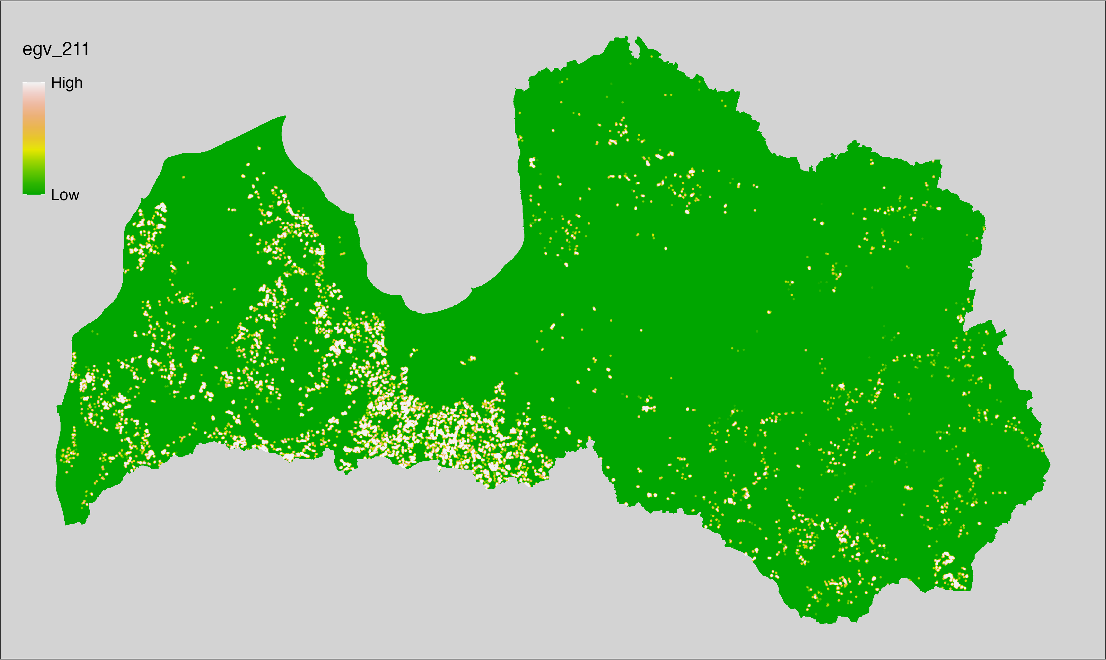
6.212 FarmlandCrops_RapeseedsWinter_r1250
filename: FarmlandCrops_RapeseedsWinter_r1250.tif
layername: egv_212
English name: Fractional cover of Winter Rapeseed, Turnip within the 1.25 km landscape
Latvian name: Ziemas rapša, ripša platības īpatsvars 1,25 km ainavā
Procedure: The cover fraction within a radius of 1250 m around the analysis grid cell
is calculated as the area-weighted sum of the analysis cells inside
the buffer, using the workflow egvtools::radius_function(). During the calculation of the landscape
metric, inverse distance weighted (power = 2) gap filling on the output is
applied to ensure no missing values at the edges. Then the layer is
rewritten to set its name. Finally, the layer is standardised by
subtracting the arithmetic mean and dividing by the root mean squared error.
Code
# libs ----
if(!require(terra)) {install.packages("terra"); require(terra)}
if(!require(egvtools)) {remotes::install_github("aavotins/egvtools"); require(egvtools)}
# Templates -----
template100=rast("./Templates/TemplateRasters/LV100m_10km.tif")
# radii ----
radius_function(
kvadrati_path = "./Templates/TemplateGrids/tiles/",
radii_path = "./Templates/TemplateGridPoints/tiles/",
tikls100_path = "./Templates/TemplateGrids/tikls100_sauzeme.parquet",
template_path = "./Templates/TemplateRasters/LV100m_10km.tif",
input_layers = c("./RasterGrids_100m/2024/RAW/FarmlandCrops_RapeseedsWinter_cell.tif"),
layer_prefixes = c("FarmlandCrops_RapeseedsWinter"),
output_dir = "./RasterGrids_100m/2024/RAW/",
n_workers = 6,
radii = c("r1250"),
radius_mode = "sparse",
extract_fun = "mean",
fill_missing = TRUE,
IDW_weight = 2,
future_max_size = 40 * 1024^3)
# FarmlandCrops_RapeseedsWinter_r1250.tif egv_212
slanis=rast("./RasterGrids_100m/2024/RAW/FarmlandCrops_RapeseedsWinter_r1250.tif")
names(slanis)="egv_212"
slanis2=project(slanis,template100)
writeRaster(slanis2,
"./RasterGrids_100m/2024/RAW/FarmlandCrops_RapeseedsWinter_r1250.tif",
overwrite=TRUE)
# standardisation ----
if(!require(terra)) {install.packages("terra"); require(terra)}
if(!require(tidyverse)) {install.packages("tidyverse"); require(tidyverse)}
nosaukums="FarmlandCrops_RapeseedsWinter_r1250.tif"
ielasisanas_cels=paste0("./RasterGrids_100m/2024/RAW/",nosaukums)
saglabasanas_cels=paste0("./RasterGrids_100m/2024/Scaled/",nosaukums)
slanis=rast(ielasisanas_cels)
videjais=global(slanis,fun="mean",na.rm=TRUE)
centrets=slanis-videjais[,1]
standartnovirze=terra::global(centrets,fun="rms",na.rm=TRUE)
merogots=centrets/standartnovirze[,1]
writeRaster(merogots,
filename=saglabasanas_cels,
overwrite=TRUE)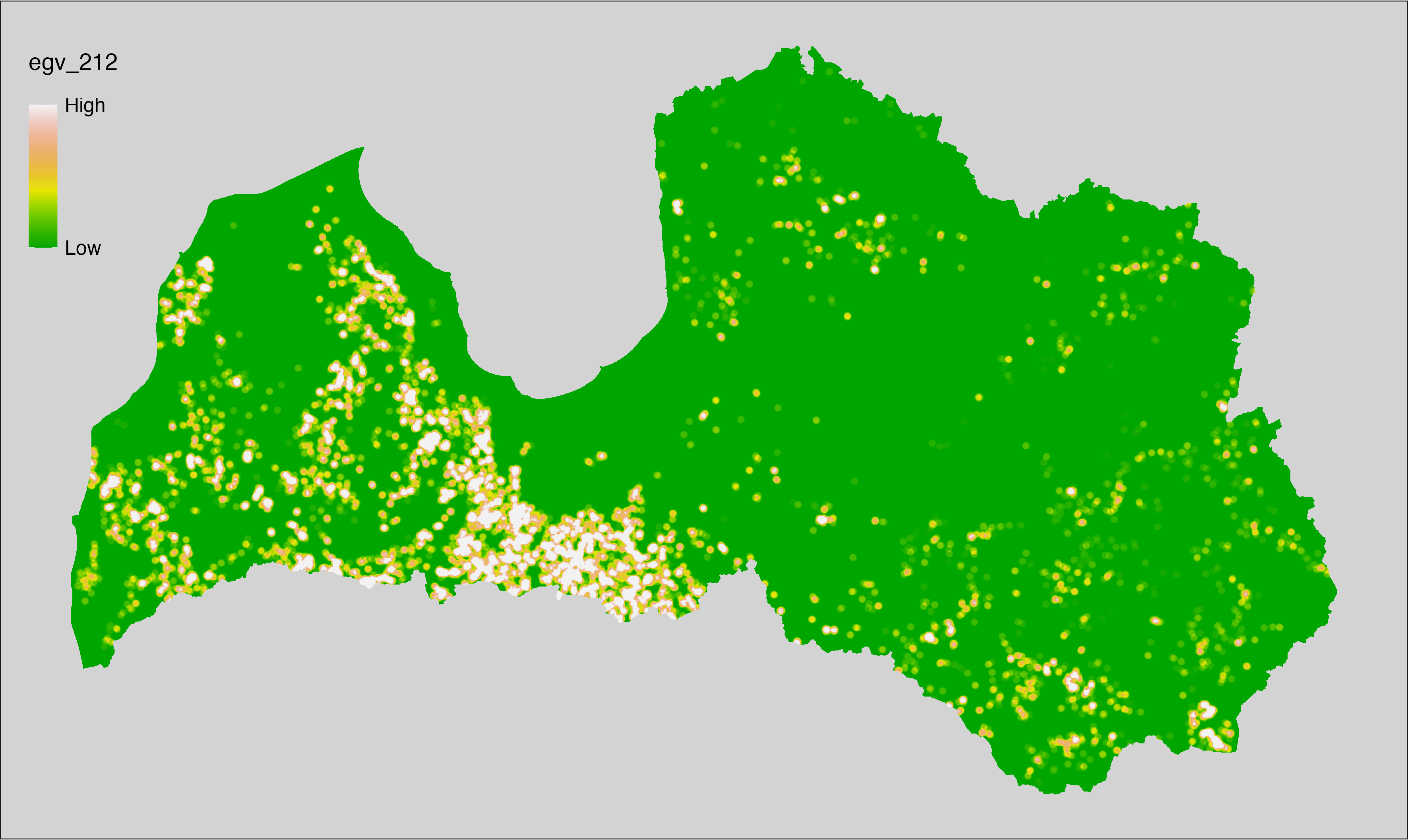
6.213 FarmlandCrops_RapeseedsWinter_r3000
filename: FarmlandCrops_RapeseedsWinter_r3000.tif
layername: egv_213
English name: Fractional cover of Winter Rapeseed, Turnip within the 3 km landscape
Latvian name: Ziemas rapša, ripša platības īpatsvars 3 km ainavā
Procedure: The cover fraction within a radius of 3000 m around the analysis grid cell
is calculated as the area-weighted sum of the analysis cells inside
the buffer, using the workflow egvtools::radius_function(). During the calculation of the landscape
metric, inverse distance weighted (power = 2) gap filling on the output is
applied to ensure no missing values at the edges. Then the layer is
rewritten to set its name. Finally, the layer is standardised by
subtracting the arithmetic mean and dividing by the root mean squared error.
Code
# libs ----
if(!require(terra)) {install.packages("terra"); require(terra)}
if(!require(egvtools)) {remotes::install_github("aavotins/egvtools"); require(egvtools)}
# Templates -----
template100=rast("./Templates/TemplateRasters/LV100m_10km.tif")
# radii ----
radius_function(
kvadrati_path = "./Templates/TemplateGrids/tiles/",
radii_path = "./Templates/TemplateGridPoints/tiles/",
tikls100_path = "./Templates/TemplateGrids/tikls100_sauzeme.parquet",
template_path = "./Templates/TemplateRasters/LV100m_10km.tif",
input_layers = c("./RasterGrids_100m/2024/RAW/FarmlandCrops_RapeseedsWinter_cell.tif"),
layer_prefixes = c("FarmlandCrops_RapeseedsWinter"),
output_dir = "./RasterGrids_100m/2024/RAW/",
n_workers = 6,
radii = c("r3000"),
radius_mode = "sparse",
extract_fun = "mean",
fill_missing = TRUE,
IDW_weight = 2,
future_max_size = 40 * 1024^3)
# FarmlandCrops_RapeseedsWinter_r3000.tif egv_213
slanis=rast("./RasterGrids_100m/2024/RAW/FarmlandCrops_RapeseedsWinter_r3000.tif")
names(slanis)="egv_213"
slanis2=project(slanis,template100)
writeRaster(slanis2,
"./RasterGrids_100m/2024/RAW/FarmlandCrops_RapeseedsWinter_r3000.tif",
overwrite=TRUE)
# standardisation ----
if(!require(terra)) {install.packages("terra"); require(terra)}
if(!require(tidyverse)) {install.packages("tidyverse"); require(tidyverse)}
nosaukums="FarmlandCrops_RapeseedsWinter_r3000.tif"
ielasisanas_cels=paste0("./RasterGrids_100m/2024/RAW/",nosaukums)
saglabasanas_cels=paste0("./RasterGrids_100m/2024/Scaled/",nosaukums)
slanis=rast(ielasisanas_cels)
videjais=global(slanis,fun="mean",na.rm=TRUE)
centrets=slanis-videjais[,1]
standartnovirze=terra::global(centrets,fun="rms",na.rm=TRUE)
merogots=centrets/standartnovirze[,1]
writeRaster(merogots,
filename=saglabasanas_cels,
overwrite=TRUE)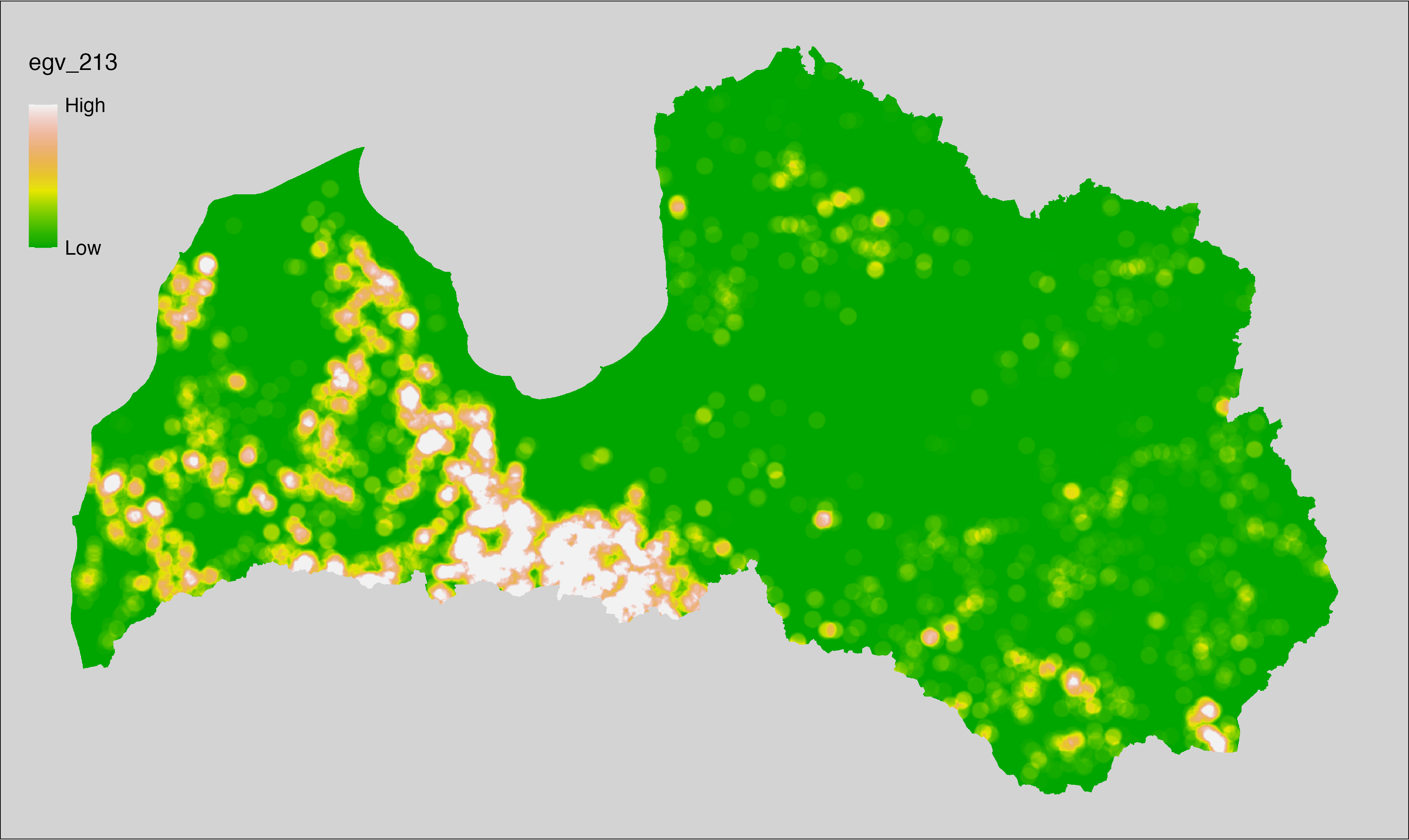
6.214 FarmlandCrops_RapeseedsWinter_r10000
filename: FarmlandCrops_RapeseedsWinter_r10000.tif
layername: egv_214
English name: Fractional cover of Winter Rapeseed, Turnip within the 10 km landscape
Latvian name: Ziemas rapša, ripša platības īpatsvars 10 km ainavā
Procedure: The cover fraction within a radius of 10000 m around the analysis grid cell
is calculated as the area-weighted sum of the analysis cells inside
the buffer, using the workflow egvtools::radius_function(). During the calculation of the landscape
metric, inverse distance weighted (power = 2) gap filling on the output is
applied to ensure no missing values at the edges. Then the layer is
rewritten to set its name. Finally, the layer is standardised by
subtracting the arithmetic mean and dividing by the root mean squared error.
Code
# libs ----
if(!require(terra)) {install.packages("terra"); require(terra)}
if(!require(egvtools)) {remotes::install_github("aavotins/egvtools"); require(egvtools)}
# Templates -----
template100=rast("./Templates/TemplateRasters/LV100m_10km.tif")
# radii ----
radius_function(
kvadrati_path = "./Templates/TemplateGrids/tiles/",
radii_path = "./Templates/TemplateGridPoints/tiles/",
tikls100_path = "./Templates/TemplateGrids/tikls100_sauzeme.parquet",
template_path = "./Templates/TemplateRasters/LV100m_10km.tif",
input_layers = c("./RasterGrids_100m/2024/RAW/FarmlandCrops_RapeseedsWinter_cell.tif"),
layer_prefixes = c("FarmlandCrops_RapeseedsWinter"),
output_dir = "./RasterGrids_100m/2024/RAW/",
n_workers = 6,
radii = c("r10000"),
radius_mode = "sparse",
extract_fun = "mean",
fill_missing = TRUE,
IDW_weight = 2,
future_max_size = 40 * 1024^3)
# FarmlandCrops_RapeseedsWinter_r10000.tif egv_214
slanis=rast("./RasterGrids_100m/2024/RAW/FarmlandCrops_RapeseedsWinter_r10000.tif")
names(slanis)="egv_214"
slanis2=project(slanis,template100)
writeRaster(slanis2,
"./RasterGrids_100m/2024/RAW/FarmlandCrops_RapeseedsWinter_r10000.tif",
overwrite=TRUE)
# standardisation ----
if(!require(terra)) {install.packages("terra"); require(terra)}
if(!require(tidyverse)) {install.packages("tidyverse"); require(tidyverse)}
nosaukums="FarmlandCrops_RapeseedsWinter_r10000.tif"
ielasisanas_cels=paste0("./RasterGrids_100m/2024/RAW/",nosaukums)
saglabasanas_cels=paste0("./RasterGrids_100m/2024/Scaled/",nosaukums)
slanis=rast(ielasisanas_cels)
videjais=global(slanis,fun="mean",na.rm=TRUE)
centrets=slanis-videjais[,1]
standartnovirze=terra::global(centrets,fun="rms",na.rm=TRUE)
merogots=centrets/standartnovirze[,1]
writeRaster(merogots,
filename=saglabasanas_cels,
overwrite=TRUE)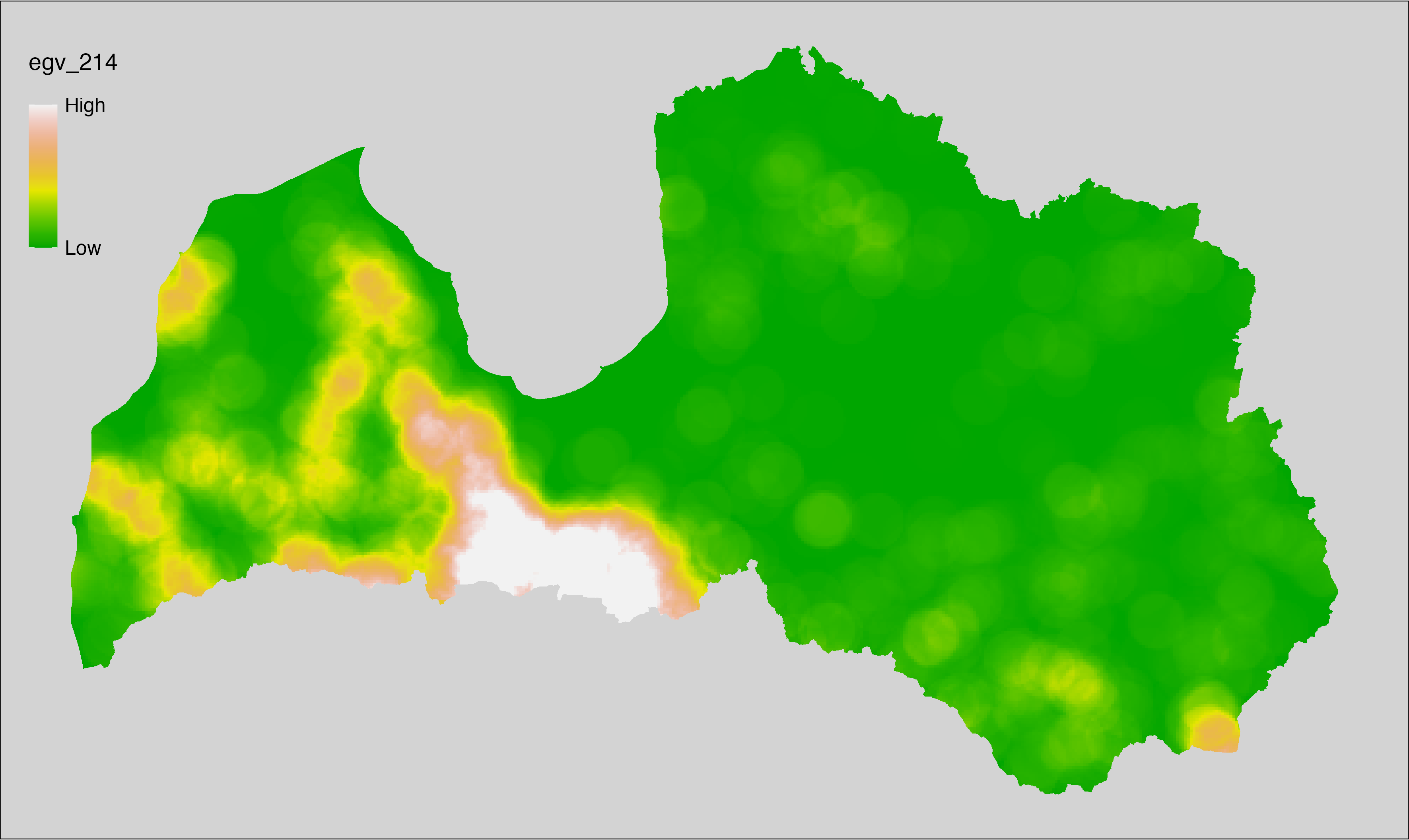
6.215 FarmlandGrassland_GrasslandsAbandoned_cell
filename: FarmlandGrassland_GrasslandsAbandoned_cell.tif
layername: egv_215
English name: Fractional cover of Abandoned Grassland within the analysis cell (1 ha)
Latvian name: Neapsaimniekotu zālāju platības īpatsvars analīzes šūnā (1 ha)
Procedure: First, the grasslands from the Landscape classification are
selected (value 330 reclassified as value 1, others as NA). Next, agricultural
parcels declared as grasslands are selected from the Rural Support Service’s
information on declared fields. Next, cells with grasslands in
Landscape classification but not in the Rural Support Service’s
information on declared fields are selected and matched to input
layer. Once matched, the layer is aggregated to EGV
resolution using the workflow egvtools::input2egv(), which calculates the arithmetic mean and thus
results in a cover fraction. During aggregation, inverse distance weighted (power = 2) gap filling
on the output is applied to ensure no missing values at the edges. Finally, the layer is standardised
by subtracting the arithmetic mean and dividing by the root mean squared error.
Code
# libs ----
if(!require(egvtools)) {remotes::install_github("aavotins/egvtools"); require(egvtools)}
if(!require(terra)) {install.packages("terra"); require(terra)}
if(!require(sf)) {install.packages("sf"); require(sf)}
if(!require(tidyverse)) {install.packages("tidyverse"); require(tidyverse)}
if(!require(sfarrow)) {install.packages("sfarrow"); require(sfarrow)}
if(!require(readxl)) {install.packages("readxl"); require(readxl)}
if(!require(raster)) {install.packages("raster"); require(raster)}
if(!require(fasterize)) {install.packages("fasterize"); require(fasterize)}
# templates ----
template100=rast("./Templates/TemplateRasters/LV100m_10km.tif")
template10=rast("./Templates/TemplateRasters/LV10m_10km.tif")
rastrs10=raster(template10)
nulls10=rast("./Templates/TemplateRasters/nulls_LV10m_10km.tif")
nulls100=rast("./Templates/TemplateRasters/nulls_LV100m_10km.tif")
# codes ----
kodi=read_excel("./Geodata/2024/LAD/KulturuKodi_2024.xlsx")
kodi$kods=as.character(kodi$kods)
# LAD ----
lad=sfarrow::st_read_parquet("./Geodata/2024/LAD/Lauki_2024.parquet")
lad$yes=1
lad=lad %>%
left_join(kodi,by=c("PRODUCT_CODE"="kods"))
# simple landscape ----
simple_landscape=rast("RasterGrids_10m/2024/Ainava_vienk_mask.tif")
# FarmlandGrassland_GrasslandsAbandoned_cell.tif egv_215 ----
landscape_grasslands=ifel(simple_landscape==330,1,0)
dati=lad %>%
filter(str_detect(SDM_grupa_sakums,"zālāji"))
table(dati$SDM_grupa_sakums,useNA="always")
lad_zalajiem=fasterize(dati,rastrs10,field="yes",fun="first")
lad_zalaji=rast(lad_zalajiem)
abandoned=ifel(landscape_grasslands==1&is.na(lad_zalaji),1,0)
plot(abandoned)
i2e_rez=egvtools::input2egv(input=abandoned,
egv_template= "./Templates/TemplateRasters/LV100m_10km.tif",
summary_function = "average",
missing_job = "FillOutput",
outlocation = "./RasterGrids_100m/2024/RAW/",
outfilename = "FarmlandGrassland_GrasslandsAbandoned_cell.tif",
layername = "egv_215",
idw_weight = 2,
plot_gaps = FALSE,plot_final = TRUE)
i2e_rez
rm(i2e_rez)
rm(dati)
rm(lad_zalajiem)
rm(lad_zalaji)
# standardisation ----
if(!require(terra)) {install.packages("terra"); require(terra)}
if(!require(tidyverse)) {install.packages("tidyverse"); require(tidyverse)}
nosaukums="FarmlandGrassland_GrasslandsAbandoned_cell.tif"
ielasisanas_cels=paste0("./RasterGrids_100m/2024/RAW/",nosaukums)
saglabasanas_cels=paste0("./RasterGrids_100m/2024/Scaled/",nosaukums)
slanis=rast(ielasisanas_cels)
videjais=global(slanis,fun="mean",na.rm=TRUE)
centrets=slanis-videjais[,1]
standartnovirze=terra::global(centrets,fun="rms",na.rm=TRUE)
merogots=centrets/standartnovirze[,1]
writeRaster(merogots,
filename=saglabasanas_cels,
overwrite=TRUE)
6.216 FarmlandGrassland_GrasslandsAbandoned_r500
filename: FarmlandGrassland_GrasslandsAbandoned_r500.tif
layername: egv_216
English name: Fractional cover of Abandoned Grassland within the 0.5 km landscape
Latvian name: Neapsaimniekotu zālāju platības īpatsvars 0,5 km ainavā
Procedure: The cover fraction within a radius of 500 m around the analysis grid cell is
calculated as the area-weighted sum of the analysis cells inside the
buffer, using the workflow egvtools::radius_function(). During the calculation of the landscape metric,
inverse distance weighted (power = 2) gap filling on the output is applied
to ensure no missing values at the edges. Then the layer is rewritten to set
its name. Finally, the layer is standardised by subtracting the arithmetic
mean and dividing by the root mean squared error.
Code
# libs ----
if(!require(terra)) {install.packages("terra"); require(terra)}
if(!require(egvtools)) {remotes::install_github("aavotins/egvtools"); require(egvtools)}
# Templates -----
template100=rast("./Templates/TemplateRasters/LV100m_10km.tif")
# radii ----
radius_function(
kvadrati_path = "./Templates/TemplateGrids/tiles/",
radii_path = "./Templates/TemplateGridPoints/tiles/",
tikls100_path = "./Templates/TemplateGrids/tikls100_sauzeme.parquet",
template_path = "./Templates/TemplateRasters/LV100m_10km.tif",
input_layers = c("./RasterGrids_100m/2024/RAW/FarmlandGrassland_GrasslandsAbandoned_cell.tif"),
layer_prefixes = c("FarmlandGrassland_GrasslandsAbandoned"),
output_dir = "./RasterGrids_100m/2024/RAW/",
n_workers = 6,
radii = c("r500"),
radius_mode = "sparse",
extract_fun = "mean",
fill_missing = TRUE,
IDW_weight = 2,
future_max_size = 40 * 1024^3)
# FarmlandGrassland_GrasslandsAbandoned_r500.tif egv_216
slanis=rast("./RasterGrids_100m/2024/RAW/FarmlandGrassland_GrasslandsAbandoned_r500.tif")
names(slanis)="egv_216"
slanis2=project(slanis,template100)
writeRaster(slanis2,
"./RasterGrids_100m/2024/RAW/FarmlandGrassland_GrasslandsAbandoned_r500.tif",
overwrite=TRUE)
# standardisation ----
if(!require(terra)) {install.packages("terra"); require(terra)}
if(!require(tidyverse)) {install.packages("tidyverse"); require(tidyverse)}
nosaukums="FarmlandGrassland_GrasslandsAbandoned_r500.tif"
ielasisanas_cels=paste0("./RasterGrids_100m/2024/RAW/",nosaukums)
saglabasanas_cels=paste0("./RasterGrids_100m/2024/Scaled/",nosaukums)
slanis=rast(ielasisanas_cels)
videjais=global(slanis,fun="mean",na.rm=TRUE)
centrets=slanis-videjais[,1]
standartnovirze=terra::global(centrets,fun="rms",na.rm=TRUE)
merogots=centrets/standartnovirze[,1]
writeRaster(merogots,
filename=saglabasanas_cels,
overwrite=TRUE)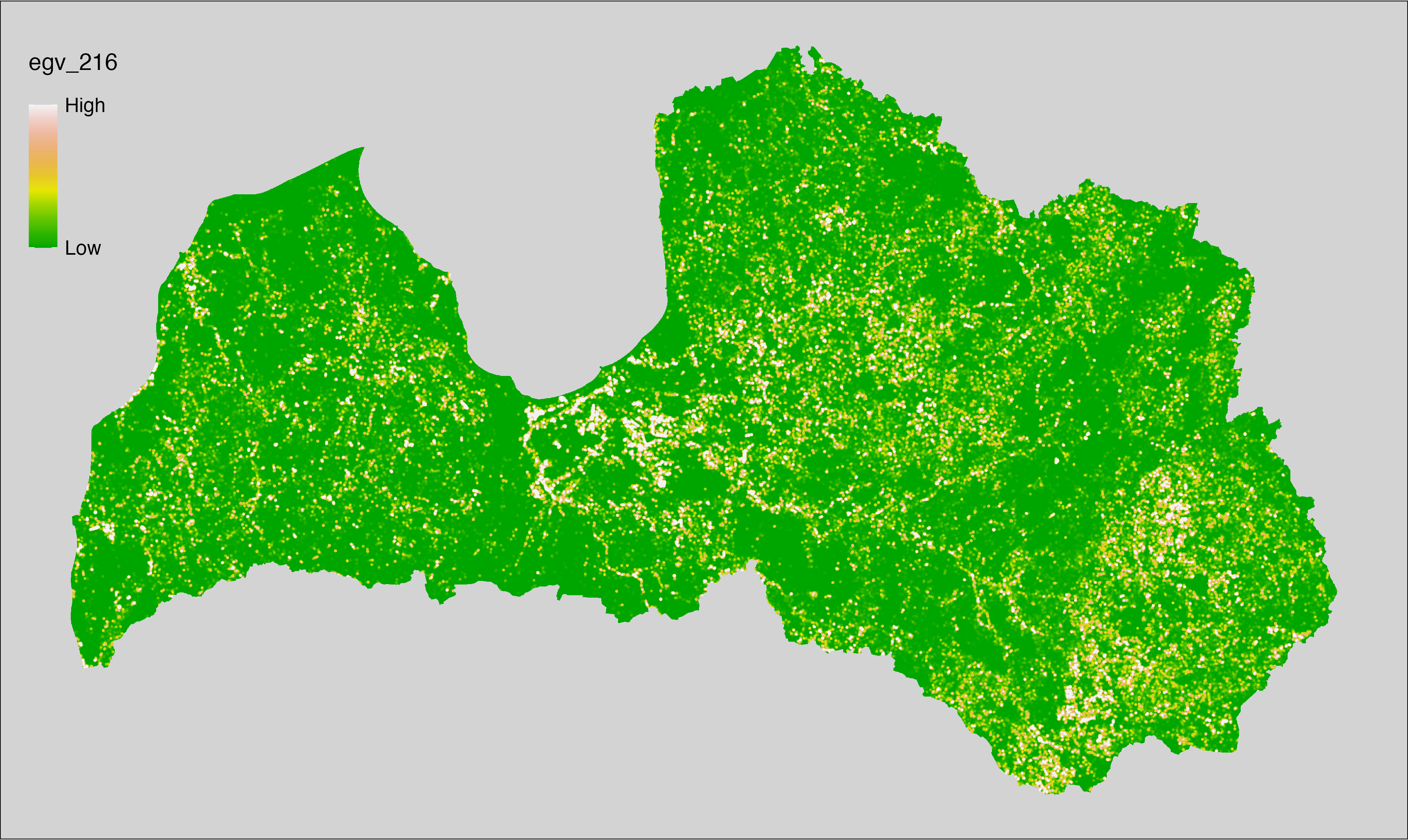
6.217 FarmlandGrassland_GrasslandsAbandoned_r1250
filename: FarmlandGrassland_GrasslandsAbandoned_r1250.tif
layername: egv_217
English name: Fractional cover of Abandoned Grassland within the 1.25 km landscape
Latvian name: Neapsaimniekotu zālāju platības īpatsvars 1,25 km ainavā
Procedure: The cover fraction within a radius of 1250 m around the analysis grid cell
is calculated as the area-weighted sum of the analysis cells inside
the buffer, using the workflow egvtools::radius_function(). During the calculation of the landscape
metric, inverse distance weighted (power = 2) gap filling on the output is
applied to ensure no missing values at the edges. Then the layer is
rewritten to set its name. Finally, the layer is standardised by
subtracting the arithmetic mean and dividing by the root mean squared error.
Code
# libs ----
if(!require(terra)) {install.packages("terra"); require(terra)}
if(!require(egvtools)) {remotes::install_github("aavotins/egvtools"); require(egvtools)}
# Templates -----
template100=rast("./Templates/TemplateRasters/LV100m_10km.tif")
# radii ----
radius_function(
kvadrati_path = "./Templates/TemplateGrids/tiles/",
radii_path = "./Templates/TemplateGridPoints/tiles/",
tikls100_path = "./Templates/TemplateGrids/tikls100_sauzeme.parquet",
template_path = "./Templates/TemplateRasters/LV100m_10km.tif",
input_layers = c("./RasterGrids_100m/2024/RAW/FarmlandGrassland_GrasslandsAbandoned_cell.tif"),
layer_prefixes = c("FarmlandGrassland_GrasslandsAbandoned"),
output_dir = "./RasterGrids_100m/2024/RAW/",
n_workers = 6,
radii = c("r1250"),
radius_mode = "sparse",
extract_fun = "mean",
fill_missing = TRUE,
IDW_weight = 2,
future_max_size = 40 * 1024^3)
# FarmlandGrassland_GrasslandsAbandoned_r1250.tif egv_217
slanis=rast("./RasterGrids_100m/2024/RAW/FarmlandGrassland_GrasslandsAbandoned_r1250.tif")
names(slanis)="egv_217"
slanis2=project(slanis,template100)
writeRaster(slanis2,
"./RasterGrids_100m/2024/RAW/FarmlandGrassland_GrasslandsAbandoned_r1250.tif",
overwrite=TRUE)
# standardisation ----
if(!require(terra)) {install.packages("terra"); require(terra)}
if(!require(tidyverse)) {install.packages("tidyverse"); require(tidyverse)}
nosaukums="FarmlandGrassland_GrasslandsAbandoned_r1250.tif"
ielasisanas_cels=paste0("./RasterGrids_100m/2024/RAW/",nosaukums)
saglabasanas_cels=paste0("./RasterGrids_100m/2024/Scaled/",nosaukums)
slanis=rast(ielasisanas_cels)
videjais=global(slanis,fun="mean",na.rm=TRUE)
centrets=slanis-videjais[,1]
standartnovirze=terra::global(centrets,fun="rms",na.rm=TRUE)
merogots=centrets/standartnovirze[,1]
writeRaster(merogots,
filename=saglabasanas_cels,
overwrite=TRUE)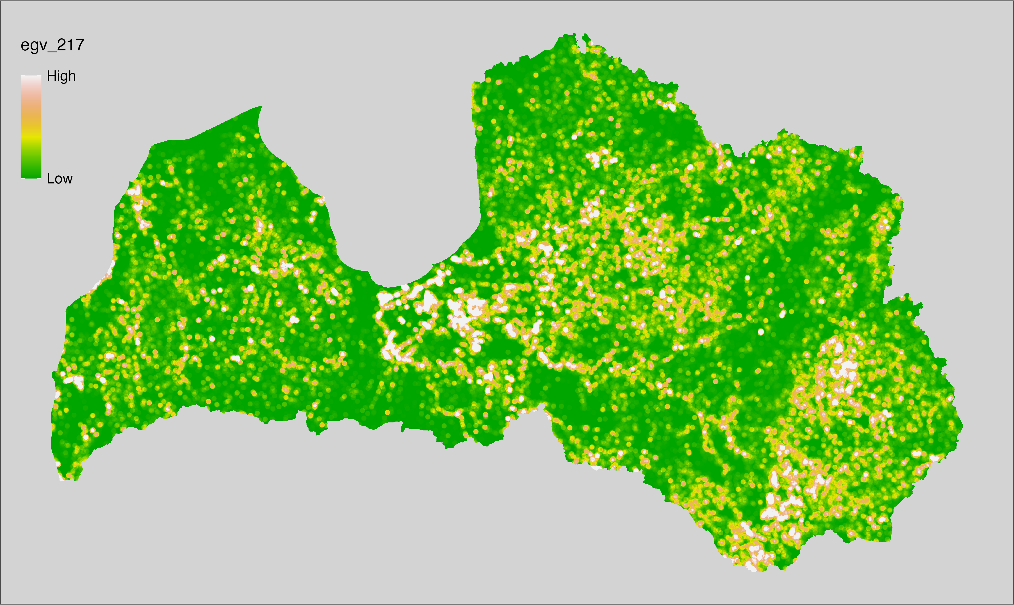
6.218 FarmlandGrassland_GrasslandsAbandoned_r3000
filename: FarmlandGrassland_GrasslandsAbandoned_r3000.tif
layername: egv_218
English name: Fractional cover of Abandoned Grassland within the 3 km landscape
Latvian name: Neapsaimniekotu zālāju platības īpatsvars 3 km ainavā
Procedure: The cover fraction within a radius of 3000 m around the analysis grid cell
is calculated as the area-weighted sum of the analysis cells inside
the buffer, using the workflow egvtools::radius_function(). During the calculation of the landscape
metric, inverse distance weighted (power = 2) gap filling on the output is
applied to ensure no missing values at the edges. Then the layer is
rewritten to set its name. Finally, the layer is standardised by
subtracting the arithmetic mean and dividing by the root mean squared error.
Code
# libs ----
if(!require(terra)) {install.packages("terra"); require(terra)}
if(!require(egvtools)) {remotes::install_github("aavotins/egvtools"); require(egvtools)}
# Templates -----
template100=rast("./Templates/TemplateRasters/LV100m_10km.tif")
# radii ----
radius_function(
kvadrati_path = "./Templates/TemplateGrids/tiles/",
radii_path = "./Templates/TemplateGridPoints/tiles/",
tikls100_path = "./Templates/TemplateGrids/tikls100_sauzeme.parquet",
template_path = "./Templates/TemplateRasters/LV100m_10km.tif",
input_layers = c("./RasterGrids_100m/2024/RAW/FarmlandGrassland_GrasslandsAbandoned_cell.tif"),
layer_prefixes = c("FarmlandGrassland_GrasslandsAbandoned"),
output_dir = "./RasterGrids_100m/2024/RAW/",
n_workers = 6,
radii = c("r3000"),
radius_mode = "sparse",
extract_fun = "mean",
fill_missing = TRUE,
IDW_weight = 2,
future_max_size = 40 * 1024^3)
# FarmlandGrassland_GrasslandsAbandoned_r3000.tif egv_218
slanis=rast("./RasterGrids_100m/2024/RAW/FarmlandGrassland_GrasslandsAbandoned_r3000.tif")
names(slanis)="egv_218"
slanis2=project(slanis,template100)
writeRaster(slanis2,
"./RasterGrids_100m/2024/RAW/FarmlandGrassland_GrasslandsAbandoned_r3000.tif",
overwrite=TRUE)
# standardisation ----
if(!require(terra)) {install.packages("terra"); require(terra)}
if(!require(tidyverse)) {install.packages("tidyverse"); require(tidyverse)}
nosaukums="FarmlandGrassland_GrasslandsAbandoned_r3000.tif"
ielasisanas_cels=paste0("./RasterGrids_100m/2024/RAW/",nosaukums)
saglabasanas_cels=paste0("./RasterGrids_100m/2024/Scaled/",nosaukums)
slanis=rast(ielasisanas_cels)
videjais=global(slanis,fun="mean",na.rm=TRUE)
centrets=slanis-videjais[,1]
standartnovirze=terra::global(centrets,fun="rms",na.rm=TRUE)
merogots=centrets/standartnovirze[,1]
writeRaster(merogots,
filename=saglabasanas_cels,
overwrite=TRUE)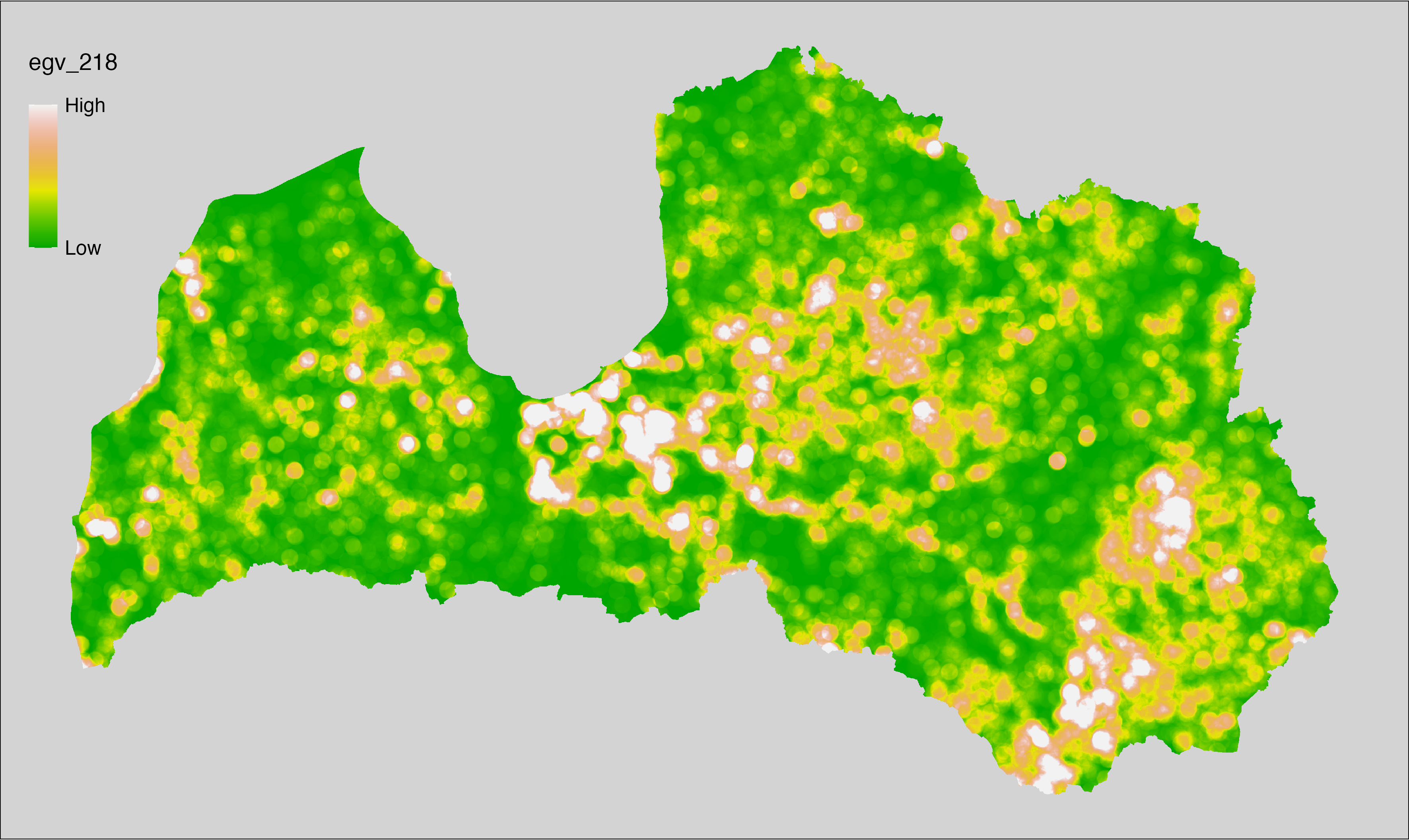
6.219 FarmlandGrassland_GrasslandsAbandoned_r10000
filename: FarmlandGrassland_GrasslandsAbandoned_r10000.tif
layername: egv_219
English name: Fractional cover of Abandoned Grassland within the 10 km landscape
Latvian name: Neapsaimniekotu zālāju platības īpatsvars 10 km ainavā
Procedure: The cover fraction within a radius of 10000 m around the analysis grid cell
is calculated as the area-weighted sum of the analysis cells inside
the buffer, using the workflow egvtools::radius_function(). During the calculation of the landscape
metric, inverse distance weighted (power = 2) gap filling on the output is
applied to ensure no missing values at the edges. Then the layer is
rewritten to set its name. Finally, the layer is standardised by
subtracting the arithmetic mean and dividing by the root mean squared error.
Code
# libs ----
if(!require(terra)) {install.packages("terra"); require(terra)}
if(!require(egvtools)) {remotes::install_github("aavotins/egvtools"); require(egvtools)}
# Templates -----
template100=rast("./Templates/TemplateRasters/LV100m_10km.tif")
# radii ----
radius_function(
kvadrati_path = "./Templates/TemplateGrids/tiles/",
radii_path = "./Templates/TemplateGridPoints/tiles/",
tikls100_path = "./Templates/TemplateGrids/tikls100_sauzeme.parquet",
template_path = "./Templates/TemplateRasters/LV100m_10km.tif",
input_layers = c("./RasterGrids_100m/2024/RAW/FarmlandGrassland_GrasslandsAbandoned_cell.tif"),
layer_prefixes = c("FarmlandGrassland_GrasslandsAbandoned"),
output_dir = "./RasterGrids_100m/2024/RAW/",
n_workers = 6,
radii = c("r10000"),
radius_mode = "sparse",
extract_fun = "mean",
fill_missing = TRUE,
IDW_weight = 2,
future_max_size = 40 * 1024^3)
# FarmlandGrassland_GrasslandsAbandoned_r10000.tif egv_219
slanis=rast("./RasterGrids_100m/2024/RAW/FarmlandGrassland_GrasslandsAbandoned_r10000.tif")
names(slanis)="egv_219"
slanis2=project(slanis,template100)
writeRaster(slanis2,
"./RasterGrids_100m/2024/RAW/FarmlandGrassland_GrasslandsAbandoned_r10000.tif",
overwrite=TRUE)
# standardisation ----
if(!require(terra)) {install.packages("terra"); require(terra)}
if(!require(tidyverse)) {install.packages("tidyverse"); require(tidyverse)}
nosaukums="FarmlandGrassland_GrasslandsAbandoned_r10000.tif"
ielasisanas_cels=paste0("./RasterGrids_100m/2024/RAW/",nosaukums)
saglabasanas_cels=paste0("./RasterGrids_100m/2024/Scaled/",nosaukums)
slanis=rast(ielasisanas_cels)
videjais=global(slanis,fun="mean",na.rm=TRUE)
centrets=slanis-videjais[,1]
standartnovirze=terra::global(centrets,fun="rms",na.rm=TRUE)
merogots=centrets/standartnovirze[,1]
writeRaster(merogots,
filename=saglabasanas_cels,
overwrite=TRUE)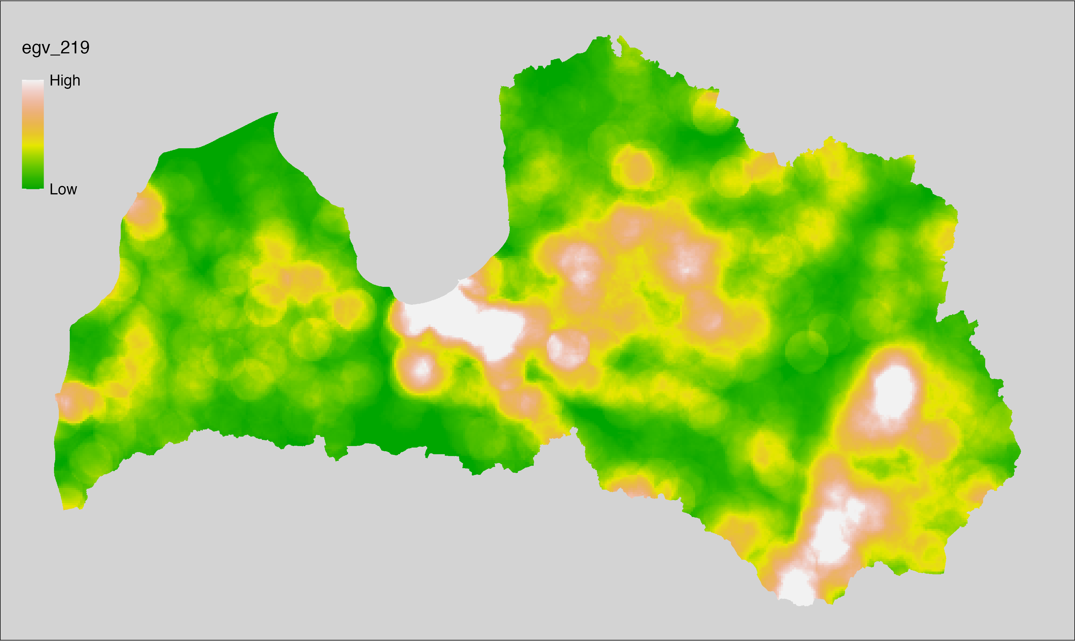
6.220 FarmlandGrassland_GrasslandsAll_cell
filename: FarmlandGrassland_GrasslandsAll_cell.tif
layername: egv_220
English name: Fractional cover of any Grassland within the analysis cell (1 ha)
Latvian name: Zālāju (visu veidu) platības īpatsvars analīzes šūnā (1 ha)
Procedure: First, the grasslands from the Landscape classification are
selected (value 330 reclassified to value 1, others as 0). Once selected, the layer
is aggregated to EGV resolution using the workflow egvtools::input2egv(), which
calculates the arithmetic mean and thus results in a cover fraction. During aggregation, inverse
distance weighted (power = 2) gap filling on the output is applied to
ensure no missing values at the edges. Finally, the layer is standardised
by subtracting the arithmetic mean and dividing by the root mean squared error.
Code
# libs ----
if(!require(egvtools)) {remotes::install_github("aavotins/egvtools"); require(egvtools)}
if(!require(terra)) {install.packages("terra"); require(terra)}
if(!require(sf)) {install.packages("sf"); require(sf)}
if(!require(tidyverse)) {install.packages("tidyverse"); require(tidyverse)}
if(!require(sfarrow)) {install.packages("sfarrow"); require(sfarrow)}
if(!require(readxl)) {install.packages("readxl"); require(readxl)}
if(!require(raster)) {install.packages("raster"); require(raster)}
if(!require(fasterize)) {install.packages("fasterize"); require(fasterize)}
# templates ----
template100=rast("./Templates/TemplateRasters/LV100m_10km.tif")
template10=rast("./Templates/TemplateRasters/LV10m_10km.tif")
rastrs10=raster(template10)
nulls10=rast("./Templates/TemplateRasters/nulls_LV10m_10km.tif")
nulls100=rast("./Templates/TemplateRasters/nulls_LV100m_10km.tif")
# codes ----
kodi=read_excel("./Geodata/2024/LAD/KulturuKodi_2024.xlsx")
kodi$kods=as.character(kodi$kods)
# LAD ----
lad=sfarrow::st_read_parquet("./Geodata/2024/LAD/Lauki_2024.parquet")
lad$yes=1
lad=lad %>%
left_join(kodi,by=c("PRODUCT_CODE"="kods"))
# simple landscape ----
simple_landscape=rast("RasterGrids_10m/2024/Ainava_vienk_mask.tif")
# FarmlandGrassland_GrasslandsAll_cell.tif egv_220 ----
landscape_grasslands=ifel(simple_landscape==330,1,0)
i2e_rez=egvtools::input2egv(input=landscape_grasslands,
egv_template= "./Templates/TemplateRasters/LV100m_10km.tif",
summary_function = "average",
missing_job = "FillOutput",
outlocation = "./RasterGrids_100m/2024/RAW/",
outfilename = "FarmlandGrassland_GrasslandsAll_cell.tif",
layername = "egv_220",
idw_weight = 2,
plot_gaps = FALSE,plot_final = TRUE)
i2e_rez
rm(i2e_rez)
rm(landscape_grasslands)
# standardisation ----
if(!require(terra)) {install.packages("terra"); require(terra)}
if(!require(tidyverse)) {install.packages("tidyverse"); require(tidyverse)}
nosaukums="FarmlandGrassland_GrasslandsAll_cell.tif"
ielasisanas_cels=paste0("./RasterGrids_100m/2024/RAW/",nosaukums)
saglabasanas_cels=paste0("./RasterGrids_100m/2024/Scaled/",nosaukums)
slanis=rast(ielasisanas_cels)
videjais=global(slanis,fun="mean",na.rm=TRUE)
centrets=slanis-videjais[,1]
standartnovirze=terra::global(centrets,fun="rms",na.rm=TRUE)
merogots=centrets/standartnovirze[,1]
writeRaster(merogots,
filename=saglabasanas_cels,
overwrite=TRUE)
6.221 FarmlandGrassland_GrasslandsAll_r500
filename: FarmlandGrassland_GrasslandsAll_r500.tif
layername: egv_221
English name: Fractional cover of any Grassland within the 0.5 km landscape
Latvian name: Zālāju (visu veidu) platības īpatsvars 0,5 km ainavā
Procedure: The cover fraction within a radius of 500 m around the analysis grid cell is
calculated as the area-weighted sum of the analysis cells inside the
buffer, using the workflow egvtools::radius_function(). During the calculation of the landscape metric,
inverse distance weighted (power = 2) gap filling on the output is applied
to ensure no missing values at the edges. Then the layer is rewritten to set
its name. Finally, the layer is standardised by subtracting the arithmetic
mean and dividing by the root mean squared error.
Code
# libs ----
if(!require(terra)) {install.packages("terra"); require(terra)}
if(!require(egvtools)) {remotes::install_github("aavotins/egvtools"); require(egvtools)}
# Templates -----
template100=rast("./Templates/TemplateRasters/LV100m_10km.tif")
# radii ----
radius_function(
kvadrati_path = "./Templates/TemplateGrids/tiles/",
radii_path = "./Templates/TemplateGridPoints/tiles/",
tikls100_path = "./Templates/TemplateGrids/tikls100_sauzeme.parquet",
template_path = "./Templates/TemplateRasters/LV100m_10km.tif",
input_layers = c("./RasterGrids_100m/2024/RAW/FarmlandGrassland_GrasslandsAll_cell.tif"),
layer_prefixes = c("FarmlandGrassland_GrasslandsAll"),
output_dir = "./RasterGrids_100m/2024/RAW/",
n_workers = 6,
radii = c("r500"),
radius_mode = "sparse",
extract_fun = "mean",
fill_missing = TRUE,
IDW_weight = 2,
future_max_size = 40 * 1024^3)
# FarmlandGrassland_GrasslandsAll_r500.tif egv_221
slanis=rast("./RasterGrids_100m/2024/RAW/FarmlandGrassland_GrasslandsAll_r500.tif")
names(slanis)="egv_221"
slanis2=project(slanis,template100)
writeRaster(slanis2,
"./RasterGrids_100m/2024/RAW/FarmlandGrassland_GrasslandsAll_r500.tif",
overwrite=TRUE)
# standardisation ----
if(!require(terra)) {install.packages("terra"); require(terra)}
if(!require(tidyverse)) {install.packages("tidyverse"); require(tidyverse)}
nosaukums="FarmlandGrassland_GrasslandsAll_r500.tif"
ielasisanas_cels=paste0("./RasterGrids_100m/2024/RAW/",nosaukums)
saglabasanas_cels=paste0("./RasterGrids_100m/2024/Scaled/",nosaukums)
slanis=rast(ielasisanas_cels)
videjais=global(slanis,fun="mean",na.rm=TRUE)
centrets=slanis-videjais[,1]
standartnovirze=terra::global(centrets,fun="rms",na.rm=TRUE)
merogots=centrets/standartnovirze[,1]
writeRaster(merogots,
filename=saglabasanas_cels,
overwrite=TRUE)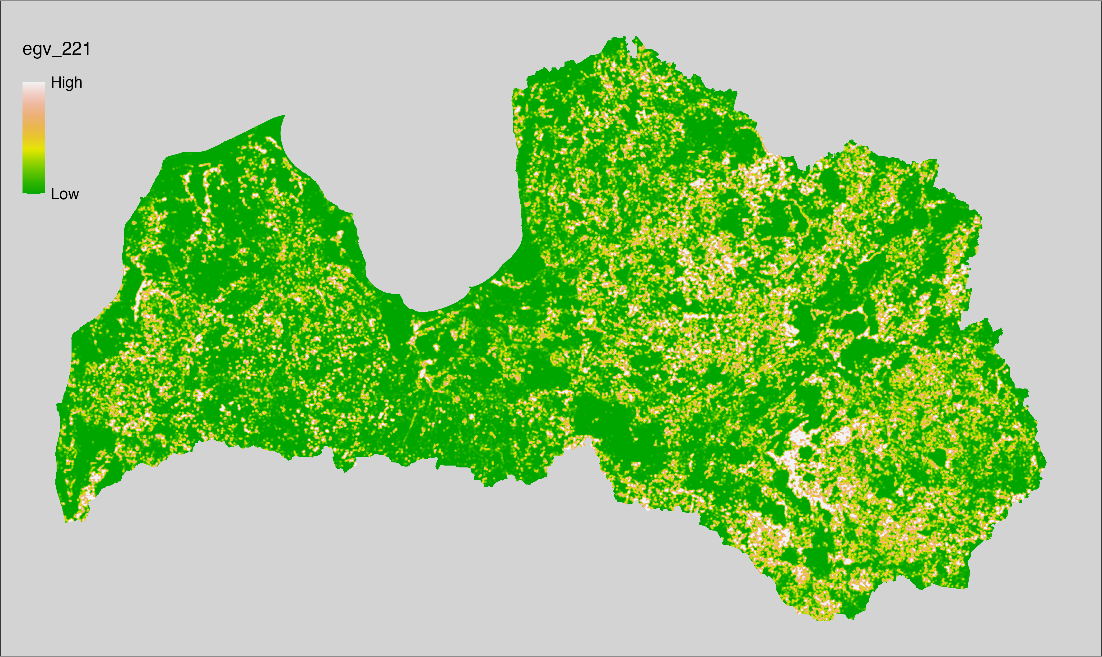
6.222 FarmlandGrassland_GrasslandsAll_r1250
filename: FarmlandGrassland_GrasslandsAll_r1250.tif
layername: egv_222
English name: Fractional cover of any Grassland within the 1.25 km landscape
Latvian name: Zālāju (visu veidu) platības īpatsvars 1,25 km ainavā
Procedure: The cover fraction within a radius of 1250 m around the analysis grid cell
is calculated as the area-weighted sum of the analysis cells inside
the buffer, using the workflow egvtools::radius_function(). During the calculation of the landscape
metric, inverse distance weighted (power = 2) gap filling on the output is
applied to ensure no missing values at the edges. Then the layer is
rewritten to set its name. Finally, the layer is standardised by
subtracting the arithmetic mean and dividing by the root mean squared error.
Code
# libs ----
if(!require(terra)) {install.packages("terra"); require(terra)}
if(!require(egvtools)) {remotes::install_github("aavotins/egvtools"); require(egvtools)}
# Templates -----
template100=rast("./Templates/TemplateRasters/LV100m_10km.tif")
# radii ----
radius_function(
kvadrati_path = "./Templates/TemplateGrids/tiles/",
radii_path = "./Templates/TemplateGridPoints/tiles/",
tikls100_path = "./Templates/TemplateGrids/tikls100_sauzeme.parquet",
template_path = "./Templates/TemplateRasters/LV100m_10km.tif",
input_layers = c("./RasterGrids_100m/2024/RAW/FarmlandGrassland_GrasslandsAll_cell.tif"),
layer_prefixes = c("FarmlandGrassland_GrasslandsAll"),
output_dir = "./RasterGrids_100m/2024/RAW/",
n_workers = 6,
radii = c("r1250"),
radius_mode = "sparse",
extract_fun = "mean",
fill_missing = TRUE,
IDW_weight = 2,
future_max_size = 40 * 1024^3)
# FarmlandGrassland_GrasslandsAll_r1250.tif egv_222
slanis=rast("./RasterGrids_100m/2024/RAW/FarmlandGrassland_GrasslandsAll_r1250.tif")
names(slanis)="egv_222"
slanis2=project(slanis,template100)
writeRaster(slanis2,
"./RasterGrids_100m/2024/RAW/FarmlandGrassland_GrasslandsAll_r1250.tif",
overwrite=TRUE)
# standardisation ----
if(!require(terra)) {install.packages("terra"); require(terra)}
if(!require(tidyverse)) {install.packages("tidyverse"); require(tidyverse)}
nosaukums="FarmlandGrassland_GrasslandsAll_r1250.tif"
ielasisanas_cels=paste0("./RasterGrids_100m/2024/RAW/",nosaukums)
saglabasanas_cels=paste0("./RasterGrids_100m/2024/Scaled/",nosaukums)
slanis=rast(ielasisanas_cels)
videjais=global(slanis,fun="mean",na.rm=TRUE)
centrets=slanis-videjais[,1]
standartnovirze=terra::global(centrets,fun="rms",na.rm=TRUE)
merogots=centrets/standartnovirze[,1]
writeRaster(merogots,
filename=saglabasanas_cels,
overwrite=TRUE)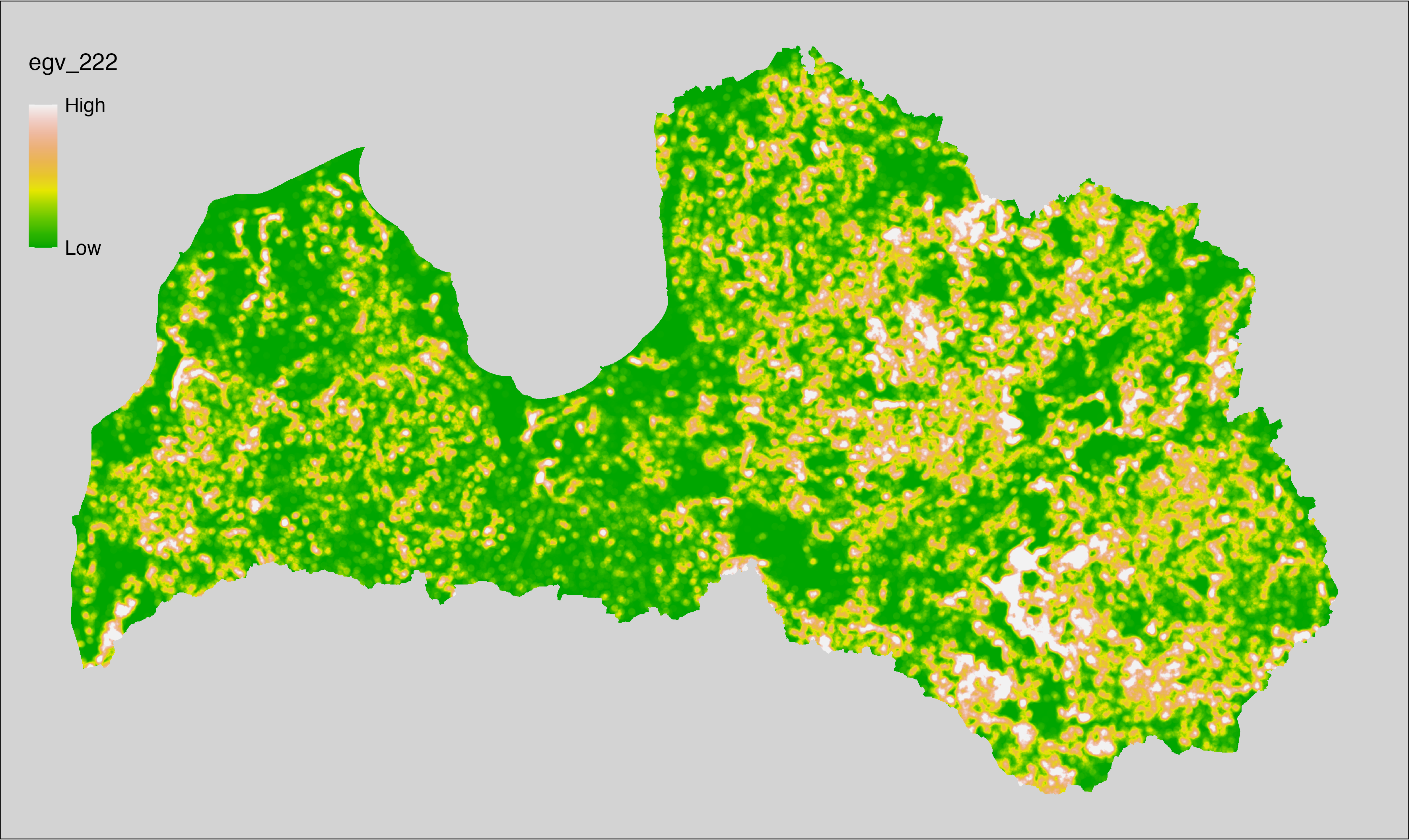
6.223 FarmlandGrassland_GrasslandsAll_r3000
filename: FarmlandGrassland_GrasslandsAll_r3000.tif
layername: egv_223
English name: Fractional cover of any Grassland within the 3 km landscape
Latvian name: Zālāju (visu veidu) platības īpatsvars 3 km ainavā
Procedure: The cover fraction within a radius of 3000 m around the analysis grid cell
is calculated as the area-weighted sum of the analysis cells inside
the buffer, using the workflow egvtools::radius_function(). During the calculation of the landscape
metric, inverse distance weighted (power = 2) gap filling on the output is
applied to ensure no missing values at the edges. Then the layer is
rewritten to set its name. Finally, the layer is standardised by
subtracting the arithmetic mean and dividing by the root mean squared error.
Code
# libs ----
if(!require(terra)) {install.packages("terra"); require(terra)}
if(!require(egvtools)) {remotes::install_github("aavotins/egvtools"); require(egvtools)}
# Templates -----
template100=rast("./Templates/TemplateRasters/LV100m_10km.tif")
# radii ----
radius_function(
kvadrati_path = "./Templates/TemplateGrids/tiles/",
radii_path = "./Templates/TemplateGridPoints/tiles/",
tikls100_path = "./Templates/TemplateGrids/tikls100_sauzeme.parquet",
template_path = "./Templates/TemplateRasters/LV100m_10km.tif",
input_layers = c("./RasterGrids_100m/2024/RAW/FarmlandGrassland_GrasslandsAll_cell.tif"),
layer_prefixes = c("FarmlandGrassland_GrasslandsAll"),
output_dir = "./RasterGrids_100m/2024/RAW/",
n_workers = 6,
radii = c("r3000"),
radius_mode = "sparse",
extract_fun = "mean",
fill_missing = TRUE,
IDW_weight = 2,
future_max_size = 40 * 1024^3)
# FarmlandGrassland_GrasslandsAll_r3000.tif egv_223
slanis=rast("./RasterGrids_100m/2024/RAW/FarmlandGrassland_GrasslandsAll_r3000.tif")
names(slanis)="egv_223"
slanis2=project(slanis,template100)
writeRaster(slanis2,
"./RasterGrids_100m/2024/RAW/FarmlandGrassland_GrasslandsAll_r3000.tif",
overwrite=TRUE)
# standardisation ----
if(!require(terra)) {install.packages("terra"); require(terra)}
if(!require(tidyverse)) {install.packages("tidyverse"); require(tidyverse)}
nosaukums="FarmlandGrassland_GrasslandsAll_r3000.tif"
ielasisanas_cels=paste0("./RasterGrids_100m/2024/RAW/",nosaukums)
saglabasanas_cels=paste0("./RasterGrids_100m/2024/Scaled/",nosaukums)
slanis=rast(ielasisanas_cels)
videjais=global(slanis,fun="mean",na.rm=TRUE)
centrets=slanis-videjais[,1]
standartnovirze=terra::global(centrets,fun="rms",na.rm=TRUE)
merogots=centrets/standartnovirze[,1]
writeRaster(merogots,
filename=saglabasanas_cels,
overwrite=TRUE)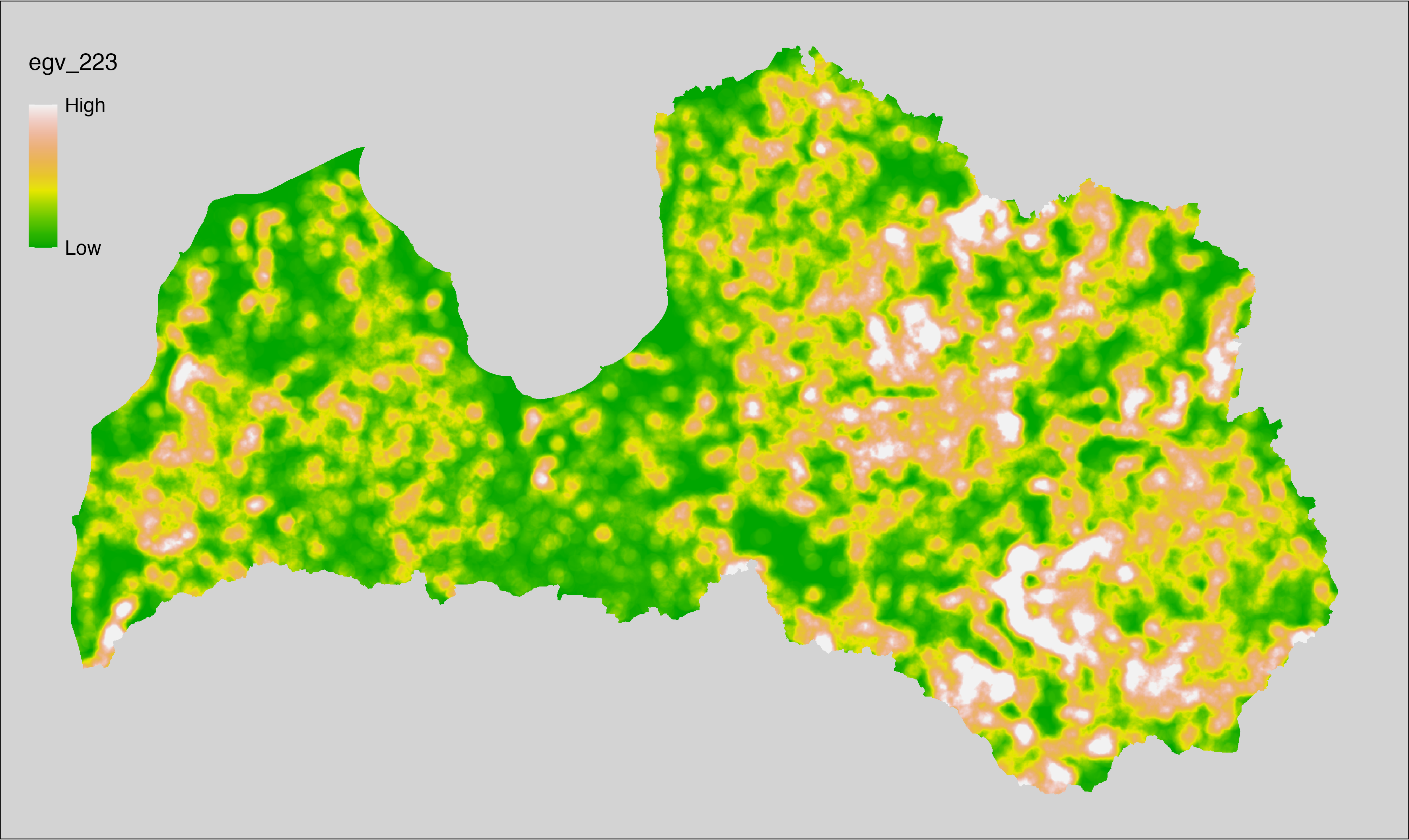
6.224 FarmlandGrassland_GrasslandsAll_r10000
filename: FarmlandGrassland_GrasslandsAll_r10000.tif
layername: egv_224
English name: Fractional cover of any Grassland within the 10 km landscape
Latvian name: Zālāju (visu veidu) platības īpatsvars 10 km ainavā
Procedure: The cover fraction within a radius of 10000 m around the analysis grid cell
is calculated as the area-weighted sum of the analysis cells inside
the buffer, using the workflow egvtools::radius_function(). During the calculation of the landscape
metric, inverse distance weighted (power = 2) gap filling on the output is
applied to ensure no missing values at the edges. Then the layer is
rewritten to set its name. Finally, the layer is standardised by
subtracting the arithmetic mean and dividing by the root mean squared error.
Code
# libs ----
if(!require(terra)) {install.packages("terra"); require(terra)}
if(!require(egvtools)) {remotes::install_github("aavotins/egvtools"); require(egvtools)}
# Templates -----
template100=rast("./Templates/TemplateRasters/LV100m_10km.tif")
# radii ----
radius_function(
kvadrati_path = "./Templates/TemplateGrids/tiles/",
radii_path = "./Templates/TemplateGridPoints/tiles/",
tikls100_path = "./Templates/TemplateGrids/tikls100_sauzeme.parquet",
template_path = "./Templates/TemplateRasters/LV100m_10km.tif",
input_layers = c("./RasterGrids_100m/2024/RAW/FarmlandGrassland_GrasslandsAll_cell.tif"),
layer_prefixes = c("FarmlandGrassland_GrasslandsAll"),
output_dir = "./RasterGrids_100m/2024/RAW/",
n_workers = 6,
radii = c("r10000"),
radius_mode = "sparse",
extract_fun = "mean",
fill_missing = TRUE,
IDW_weight = 2,
future_max_size = 40 * 1024^3)
# FarmlandGrassland_GrasslandsAll_r10000.tif egv_224
slanis=rast("./RasterGrids_100m/2024/RAW/FarmlandGrassland_GrasslandsAll_r10000.tif")
names(slanis)="egv_224"
slanis2=project(slanis,template100)
writeRaster(slanis2,
"./RasterGrids_100m/2024/RAW/FarmlandGrassland_GrasslandsAll_r10000.tif",
overwrite=TRUE)
# standardisation ----
if(!require(terra)) {install.packages("terra"); require(terra)}
if(!require(tidyverse)) {install.packages("tidyverse"); require(tidyverse)}
nosaukums="FarmlandGrassland_GrasslandsAll_r10000.tif"
ielasisanas_cels=paste0("./RasterGrids_100m/2024/RAW/",nosaukums)
saglabasanas_cels=paste0("./RasterGrids_100m/2024/Scaled/",nosaukums)
slanis=rast(ielasisanas_cels)
videjais=global(slanis,fun="mean",na.rm=TRUE)
centrets=slanis-videjais[,1]
standartnovirze=terra::global(centrets,fun="rms",na.rm=TRUE)
merogots=centrets/standartnovirze[,1]
writeRaster(merogots,
filename=saglabasanas_cels,
overwrite=TRUE)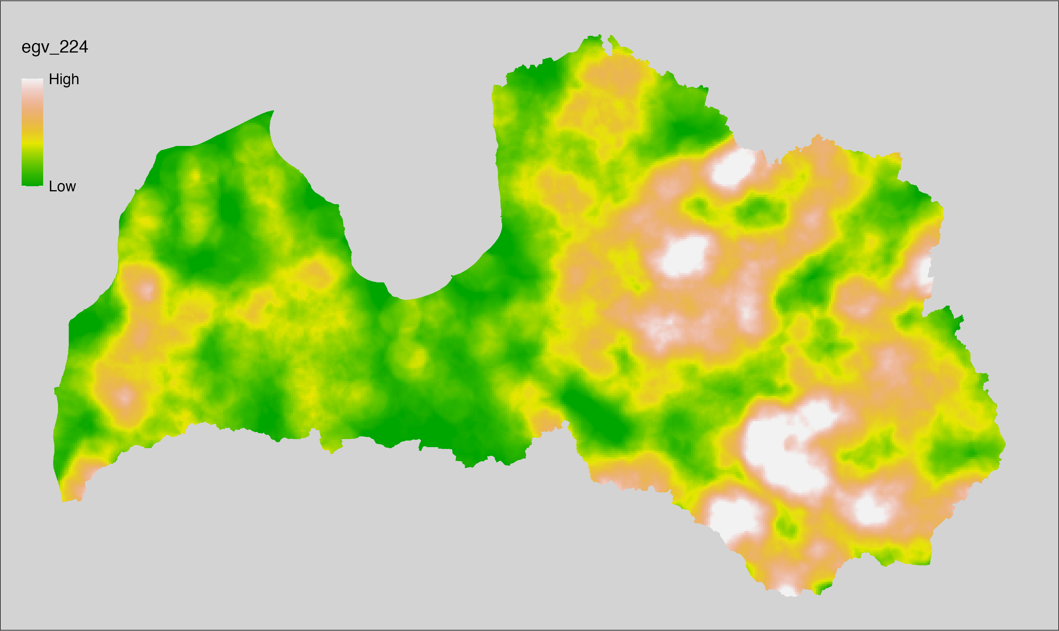
6.225 FarmlandGrassland_GrasslandsPermanent_cell
filename: FarmlandGrassland_GrasslandsPermanent_cell.tif
layername: egv_225
English name: Fractional cover of Permanent Grassland within the analysis cell (1 ha)
Latvian name: Ilggadīgu zālāju platības īpatsvars analīzes šūnā (1 ha)
Procedure: First, agricultural parcels declared as permanent grasslands are
selected from the Rural Support Service’s information on declared
fields. These geometries are then rasterised to input resolution,
ensuring value 1 at the polygon locations and value 0 elsewhere. Rasterisation
is performed with the workflow egvtools::polygon2input(). Once rasterised, the layer is
aggregated to EGV resolution using the workflow egvtools::input2egv(), which
calculates the arithmetic mean and thus results in a cover fraction. During aggregation, inverse
distance weighted (power = 2) gap filling on the output is applied to
ensure no missing values at the edges. Finally, the layer is standardised
by subtracting the arithmetic mean and dividing by the root mean squared error.
Code
# libs ----
if(!require(egvtools)) {remotes::install_github("aavotins/egvtools"); require(egvtools)}
if(!require(terra)) {install.packages("terra"); require(terra)}
if(!require(sf)) {install.packages("sf"); require(sf)}
if(!require(tidyverse)) {install.packages("tidyverse"); require(tidyverse)}
if(!require(sfarrow)) {install.packages("sfarrow"); require(sfarrow)}
if(!require(readxl)) {install.packages("readxl"); require(readxl)}
if(!require(raster)) {install.packages("raster"); require(raster)}
if(!require(fasterize)) {install.packages("fasterize"); require(fasterize)}
# templates ----
template100=rast("./Templates/TemplateRasters/LV100m_10km.tif")
template10=rast("./Templates/TemplateRasters/LV10m_10km.tif")
rastrs10=raster(template10)
nulls10=rast("./Templates/TemplateRasters/nulls_LV10m_10km.tif")
nulls100=rast("./Templates/TemplateRasters/nulls_LV100m_10km.tif")
# codes ----
kodi=read_excel("./Geodata/2024/LAD/KulturuKodi_2024.xlsx")
kodi$kods=as.character(kodi$kods)
# LAD ----
lad=sfarrow::st_read_parquet("./Geodata/2024/LAD/Lauki_2024.parquet")
lad$yes=1
lad=lad %>%
left_join(kodi,by=c("PRODUCT_CODE"="kods"))
# simple landscape ----
simple_landscape=rast("RasterGrids_10m/2024/Ainava_vienk_mask.tif")
# FarmlandGrassland_GrasslandsPermanent_cell.tif egv_225 ----
dati=lad %>%
filter(SDM_grupa_sakums=="zālāji (ilggadīgie)")
table(dati$SDM_grupa_sakums,useNA="always")
p2i_rez=egvtools::polygon2input(vector_data = dati,
template_path = "./Templates/TemplateRasters/LV10m_10km.tif",
out_path = "./RasterGrids_10m/2024/",
file_name = "FarmlandGrassland_GrasslandsPermanent_input.tif",
value_field = "yes",
prepare=FALSE,
background_raster = "./Templates/TemplateRasters/nulls_LV10m_10km.tif",
plot_result = TRUE)
p2i_rez
i2e_rez=egvtools::input2egv(input=paste0("./RasterGrids_10m/2024/",
"FarmlandGrassland_GrasslandsPermanent_input.tif"),
egv_template= "./Templates/TemplateRasters/LV100m_10km.tif",
summary_function = "average",
missing_job = "FillOutput",
outlocation = "./RasterGrids_100m/2024/RAW/",
outfilename = "FarmlandGrassland_GrasslandsPermanent_cell.tif",
layername = "egv_225",
idw_weight = 2,
plot_gaps = FALSE,plot_final = TRUE)
i2e_rez
rm(p2i_rez)
rm(i2e_rez)
rm(dati)
unlink("./RasterGrids_10m/2024/FarmlandGrassland_GrasslandsPermanent_input.tif")
# standardisation ----
if(!require(terra)) {install.packages("terra"); require(terra)}
if(!require(tidyverse)) {install.packages("tidyverse"); require(tidyverse)}
nosaukums="FarmlandGrassland_GrasslandsPermanent_cell.tif"
ielasisanas_cels=paste0("./RasterGrids_100m/2024/RAW/",nosaukums)
saglabasanas_cels=paste0("./RasterGrids_100m/2024/Scaled/",nosaukums)
slanis=rast(ielasisanas_cels)
videjais=global(slanis,fun="mean",na.rm=TRUE)
centrets=slanis-videjais[,1]
standartnovirze=terra::global(centrets,fun="rms",na.rm=TRUE)
merogots=centrets/standartnovirze[,1]
writeRaster(merogots,
filename=saglabasanas_cels,
overwrite=TRUE)
6.226 FarmlandGrassland_GrasslandsPermanent_r500
filename: FarmlandGrassland_GrasslandsPermanent_r500.tif
layername: egv_226
English name: Fractional cover of Permanent Grassland within the 0.5 km landscape
Latvian name: Ilggadīgu zālāju platības īpatsvars 0,5 km ainavā
Procedure: The cover fraction within a radius of 500 m around the analysis grid cell is
calculated as the area-weighted sum of the analysis cells inside the
buffer, using the workflow egvtools::radius_function(). During the calculation of the landscape metric,
inverse distance weighted (power = 2) gap filling on the output is applied
to ensure no missing values at the edges. Then the layer is rewritten to set
its name. Finally, the layer is standardised by subtracting the arithmetic
mean and dividing by the root mean squared error.
Code
# libs ----
if(!require(terra)) {install.packages("terra"); require(terra)}
if(!require(egvtools)) {remotes::install_github("aavotins/egvtools"); require(egvtools)}
# Templates -----
template100=rast("./Templates/TemplateRasters/LV100m_10km.tif")
# radii ----
radius_function(
kvadrati_path = "./Templates/TemplateGrids/tiles/",
radii_path = "./Templates/TemplateGridPoints/tiles/",
tikls100_path = "./Templates/TemplateGrids/tikls100_sauzeme.parquet",
template_path = "./Templates/TemplateRasters/LV100m_10km.tif",
input_layers = c("./RasterGrids_100m/2024/RAW/FarmlandGrassland_GrasslandsPermanent_cell.tif"),
layer_prefixes = c("FarmlandGrassland_GrasslandsPermanent"),
output_dir = "./RasterGrids_100m/2024/RAW/",
n_workers = 6,
radii = c("r500"),
radius_mode = "sparse",
extract_fun = "mean",
fill_missing = TRUE,
IDW_weight = 2,
future_max_size = 40 * 1024^3)
# FarmlandGrassland_GrasslandsPermanent_r500.tif egv_226
slanis=rast("./RasterGrids_100m/2024/RAW/FarmlandGrassland_GrasslandsPermanent_r500.tif")
names(slanis)="egv_226"
slanis2=project(slanis,template100)
writeRaster(slanis2,
"./RasterGrids_100m/2024/RAW/FarmlandGrassland_GrasslandsPermanent_r500.tif",
overwrite=TRUE)
# standardisation ----
if(!require(terra)) {install.packages("terra"); require(terra)}
if(!require(tidyverse)) {install.packages("tidyverse"); require(tidyverse)}
nosaukums="FarmlandGrassland_GrasslandsPermanent_r500.tif"
ielasisanas_cels=paste0("./RasterGrids_100m/2024/RAW/",nosaukums)
saglabasanas_cels=paste0("./RasterGrids_100m/2024/Scaled/",nosaukums)
slanis=rast(ielasisanas_cels)
videjais=global(slanis,fun="mean",na.rm=TRUE)
centrets=slanis-videjais[,1]
standartnovirze=terra::global(centrets,fun="rms",na.rm=TRUE)
merogots=centrets/standartnovirze[,1]
writeRaster(merogots,
filename=saglabasanas_cels,
overwrite=TRUE)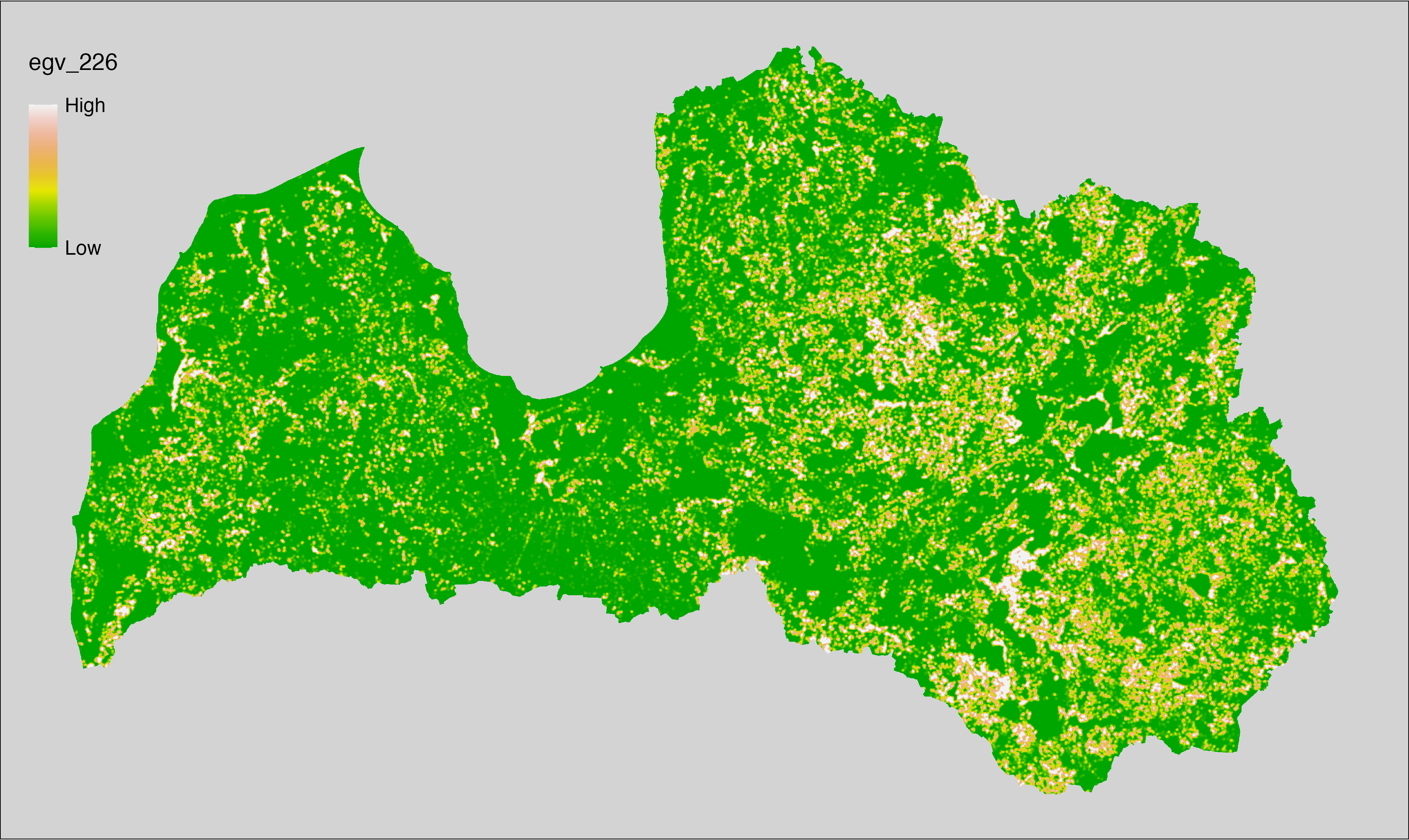
6.227 FarmlandGrassland_GrasslandsPermanent_r1250
filename: FarmlandGrassland_GrasslandsPermanent_r1250.tif
layername: egv_227
English name: Fractional cover of Permanent Grassland within the 1.25 km landscape
Latvian name: Ilggadīgu zālāju platības īpatsvars 1,25 km ainavā
Procedure: The cover fraction within a radius of 1250 m around the analysis grid cell
is calculated as the area-weighted sum of the analysis cells inside
the buffer, using the workflow egvtools::radius_function(). During the calculation of the landscape
metric, inverse distance weighted (power = 2) gap filling on the output is
applied to ensure no missing values at the edges. Then the layer is
rewritten to set its name. Finally, the layer is standardised by
subtracting the arithmetic mean and dividing by the root mean squared error.
Code
# libs ----
if(!require(terra)) {install.packages("terra"); require(terra)}
if(!require(egvtools)) {remotes::install_github("aavotins/egvtools"); require(egvtools)}
# Templates -----
template100=rast("./Templates/TemplateRasters/LV100m_10km.tif")
# radii ----
radius_function(
kvadrati_path = "./Templates/TemplateGrids/tiles/",
radii_path = "./Templates/TemplateGridPoints/tiles/",
tikls100_path = "./Templates/TemplateGrids/tikls100_sauzeme.parquet",
template_path = "./Templates/TemplateRasters/LV100m_10km.tif",
input_layers = c("./RasterGrids_100m/2024/RAW/FarmlandGrassland_GrasslandsPermanent_cell.tif"),
layer_prefixes = c("FarmlandGrassland_GrasslandsPermanent"),
output_dir = "./RasterGrids_100m/2024/RAW/",
n_workers = 6,
radii = c("r1250"),
radius_mode = "sparse",
extract_fun = "mean",
fill_missing = TRUE,
IDW_weight = 2,
future_max_size = 40 * 1024^3)
# FarmlandGrassland_GrasslandsPermanent_r1250.tif egv_227
slanis=rast("./RasterGrids_100m/2024/RAW/FarmlandGrassland_GrasslandsPermanent_r1250.tif")
names(slanis)="egv_227"
slanis2=project(slanis,template100)
writeRaster(slanis2,
"./RasterGrids_100m/2024/RAW/FarmlandGrassland_GrasslandsPermanent_r1250.tif",
overwrite=TRUE)
# standardisation ----
if(!require(terra)) {install.packages("terra"); require(terra)}
if(!require(tidyverse)) {install.packages("tidyverse"); require(tidyverse)}
nosaukums="FarmlandGrassland_GrasslandsPermanent_r1250.tif"
ielasisanas_cels=paste0("./RasterGrids_100m/2024/RAW/",nosaukums)
saglabasanas_cels=paste0("./RasterGrids_100m/2024/Scaled/",nosaukums)
slanis=rast(ielasisanas_cels)
videjais=global(slanis,fun="mean",na.rm=TRUE)
centrets=slanis-videjais[,1]
standartnovirze=terra::global(centrets,fun="rms",na.rm=TRUE)
merogots=centrets/standartnovirze[,1]
writeRaster(merogots,
filename=saglabasanas_cels,
overwrite=TRUE)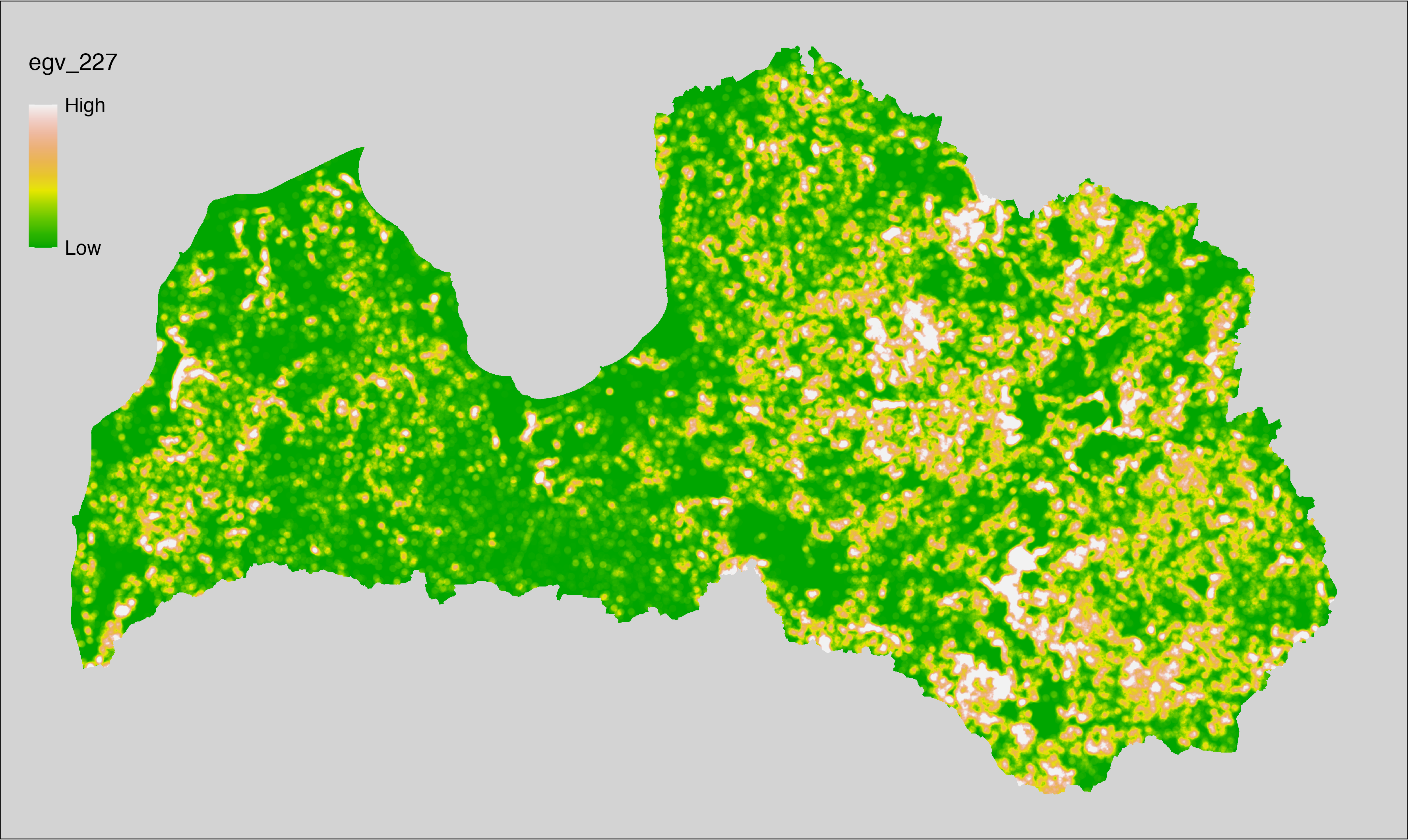
6.228 FarmlandGrassland_GrasslandsPermanent_r3000
filename: FarmlandGrassland_GrasslandsPermanent_r3000.tif
layername: egv_228
English name: Fractional cover of Permanent Grassland within the 3 km landscape
Latvian name: Ilggadīgu zālāju platības īpatsvars 3 km ainavā
Procedure: The cover fraction within a radius of 3000 m around the analysis grid cell
is calculated as the area-weighted sum of the analysis cells inside
the buffer, using the workflow egvtools::radius_function(). During the calculation of the landscape
metric, inverse distance weighted (power = 2) gap filling on the output is
applied to ensure no missing values at the edges. Then the layer is
rewritten to set its name. Finally, the layer is standardised by
subtracting the arithmetic mean and dividing by the root mean squared error.
Code
# libs ----
if(!require(terra)) {install.packages("terra"); require(terra)}
if(!require(egvtools)) {remotes::install_github("aavotins/egvtools"); require(egvtools)}
# Templates -----
template100=rast("./Templates/TemplateRasters/LV100m_10km.tif")
# radii ----
radius_function(
kvadrati_path = "./Templates/TemplateGrids/tiles/",
radii_path = "./Templates/TemplateGridPoints/tiles/",
tikls100_path = "./Templates/TemplateGrids/tikls100_sauzeme.parquet",
template_path = "./Templates/TemplateRasters/LV100m_10km.tif",
input_layers = c("./RasterGrids_100m/2024/RAW/FarmlandGrassland_GrasslandsPermanent_cell.tif"),
layer_prefixes = c("FarmlandGrassland_GrasslandsPermanent"),
output_dir = "./RasterGrids_100m/2024/RAW/",
n_workers = 6,
radii = c("r3000"),
radius_mode = "sparse",
extract_fun = "mean",
fill_missing = TRUE,
IDW_weight = 2,
future_max_size = 40 * 1024^3)
# FarmlandGrassland_GrasslandsPermanent_r3000.tif egv_228
slanis=rast("./RasterGrids_100m/2024/RAW/FarmlandGrassland_GrasslandsPermanent_r3000.tif")
names(slanis)="egv_228"
slanis2=project(slanis,template100)
writeRaster(slanis2,
"./RasterGrids_100m/2024/RAW/FarmlandGrassland_GrasslandsPermanent_r3000.tif",
overwrite=TRUE)
# standardisation ----
if(!require(terra)) {install.packages("terra"); require(terra)}
if(!require(tidyverse)) {install.packages("tidyverse"); require(tidyverse)}
nosaukums="FarmlandGrassland_GrasslandsPermanent_r3000.tif"
ielasisanas_cels=paste0("./RasterGrids_100m/2024/RAW/",nosaukums)
saglabasanas_cels=paste0("./RasterGrids_100m/2024/Scaled/",nosaukums)
slanis=rast(ielasisanas_cels)
videjais=global(slanis,fun="mean",na.rm=TRUE)
centrets=slanis-videjais[,1]
standartnovirze=terra::global(centrets,fun="rms",na.rm=TRUE)
merogots=centrets/standartnovirze[,1]
writeRaster(merogots,
filename=saglabasanas_cels,
overwrite=TRUE)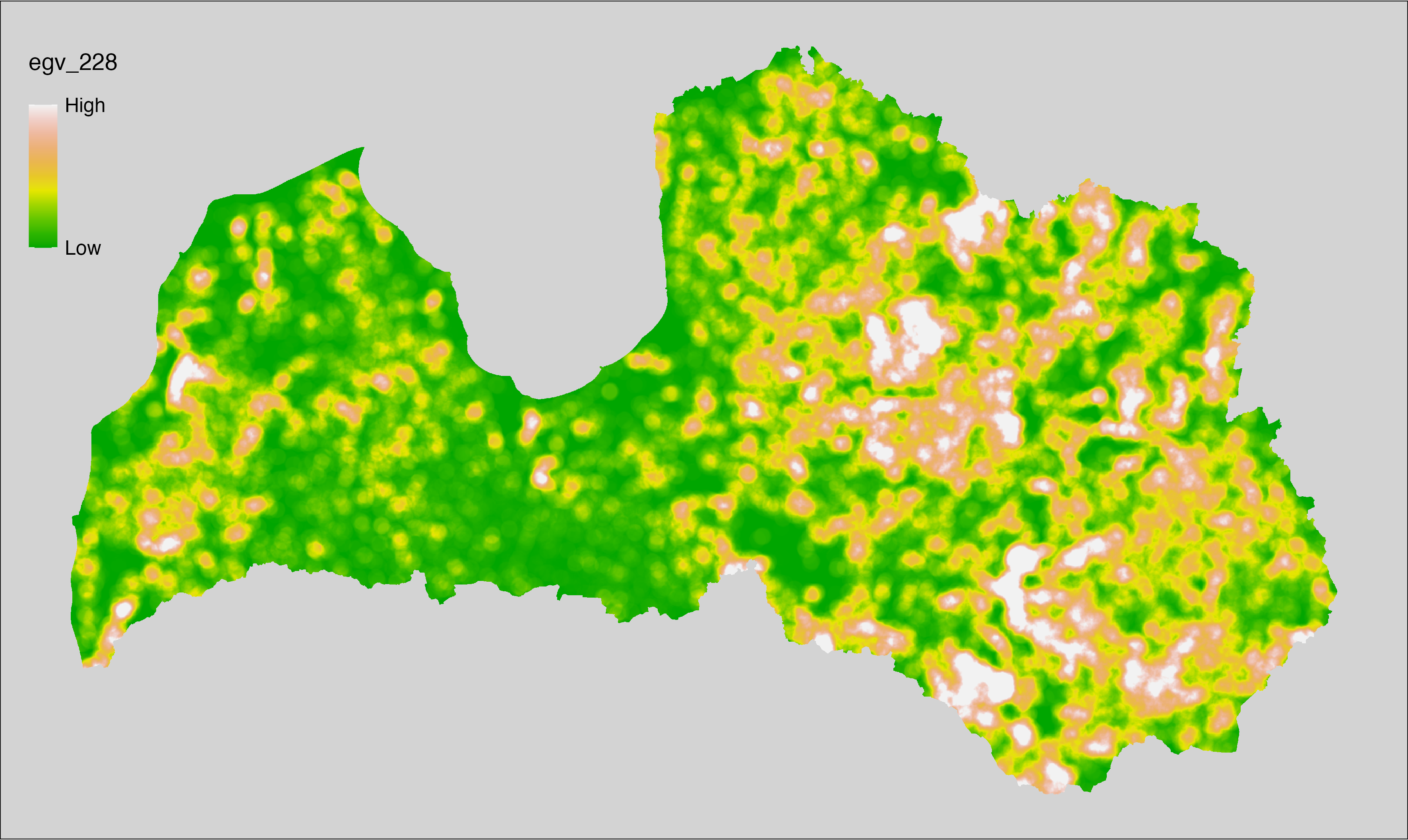
6.229 FarmlandGrassland_GrasslandsPermanent_r10000
filename: FarmlandGrassland_GrasslandsPermanent_r10000.tif
layername: egv_229
English name: Fractional cover of Permanent Grassland within the 10 km landscape
Latvian name: Ilggadīgu zālāju platības īpatsvars 10 km ainavā
Procedure: The cover fraction within a radius of 10000 m around the analysis grid cell
is calculated as the area-weighted sum of the analysis cells inside
the buffer, using the workflow egvtools::radius_function(). During the calculation of the landscape
metric, inverse distance weighted (power = 2) gap filling on the output is
applied to ensure no missing values at the edges. Then the layer is
rewritten to set its name. Finally, the layer is standardised by
subtracting the arithmetic mean and dividing by the root mean squared error.
Code
# libs ----
if(!require(terra)) {install.packages("terra"); require(terra)}
if(!require(egvtools)) {remotes::install_github("aavotins/egvtools"); require(egvtools)}
# Templates -----
template100=rast("./Templates/TemplateRasters/LV100m_10km.tif")
# radii ----
radius_function(
kvadrati_path = "./Templates/TemplateGrids/tiles/",
radii_path = "./Templates/TemplateGridPoints/tiles/",
tikls100_path = "./Templates/TemplateGrids/tikls100_sauzeme.parquet",
template_path = "./Templates/TemplateRasters/LV100m_10km.tif",
input_layers = c("./RasterGrids_100m/2024/RAW/FarmlandGrassland_GrasslandsPermanent_cell.tif"),
layer_prefixes = c("FarmlandGrassland_GrasslandsPermanent"),
output_dir = "./RasterGrids_100m/2024/RAW/",
n_workers = 6,
radii = c("r10000"),
radius_mode = "sparse",
extract_fun = "mean",
fill_missing = TRUE,
IDW_weight = 2,
future_max_size = 40 * 1024^3)
# FarmlandGrassland_GrasslandsPermanent_r10000.tif egv_229
slanis=rast("./RasterGrids_100m/2024/RAW/FarmlandGrassland_GrasslandsPermanent_r10000.tif")
names(slanis)="egv_229"
slanis2=project(slanis,template100)
writeRaster(slanis2,
"./RasterGrids_100m/2024/RAW/FarmlandGrassland_GrasslandsPermanent_r10000.tif",
overwrite=TRUE)
# standardisation ----
if(!require(terra)) {install.packages("terra"); require(terra)}
if(!require(tidyverse)) {install.packages("tidyverse"); require(tidyverse)}
nosaukums="FarmlandGrassland_GrasslandsPermanent_r10000.tif"
ielasisanas_cels=paste0("./RasterGrids_100m/2024/RAW/",nosaukums)
saglabasanas_cels=paste0("./RasterGrids_100m/2024/Scaled/",nosaukums)
slanis=rast(ielasisanas_cels)
videjais=global(slanis,fun="mean",na.rm=TRUE)
centrets=slanis-videjais[,1]
standartnovirze=terra::global(centrets,fun="rms",na.rm=TRUE)
merogots=centrets/standartnovirze[,1]
writeRaster(merogots,
filename=saglabasanas_cels,
overwrite=TRUE)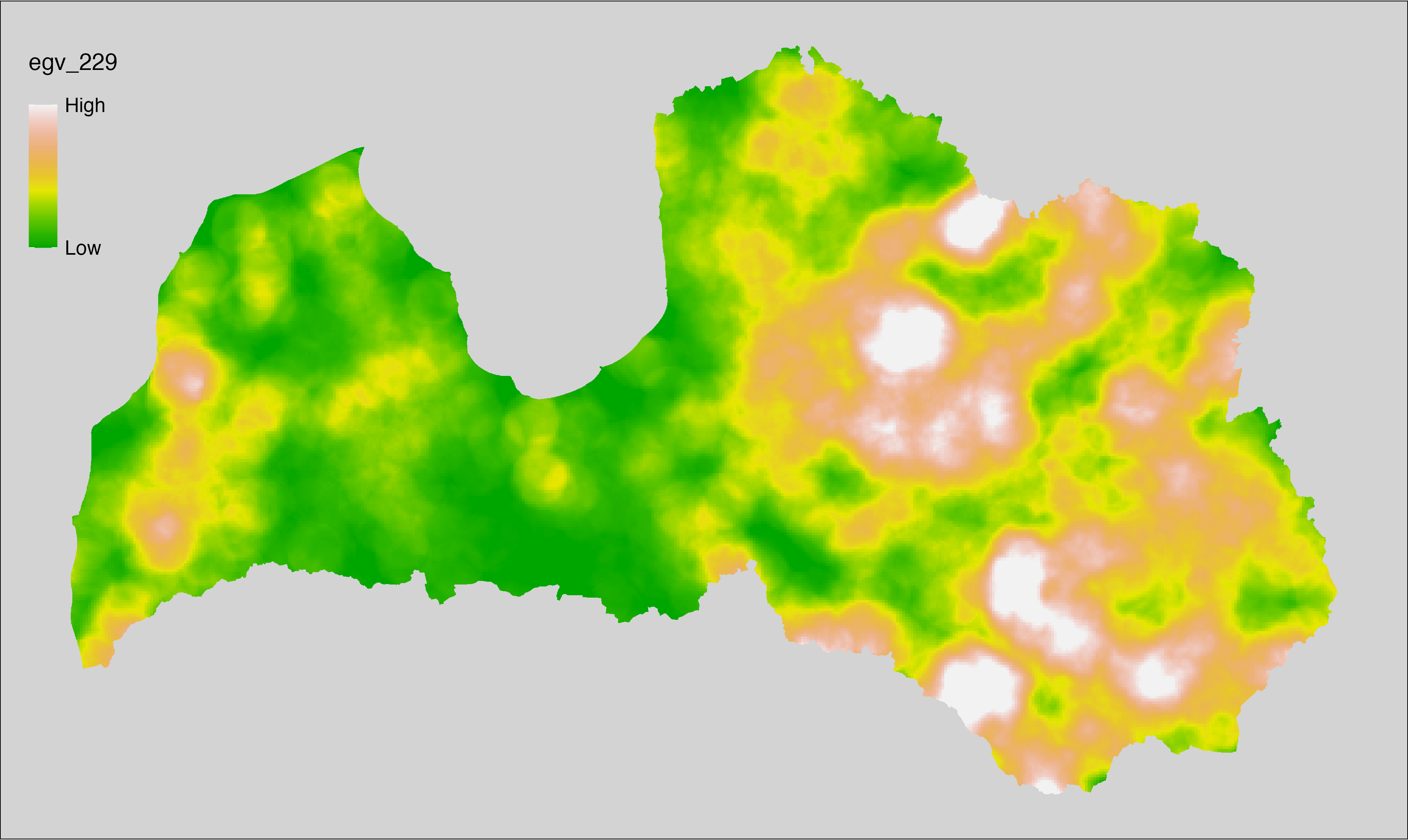
6.230 FarmlandGrassland_GrasslandsTemporary_cell
filename: FarmlandGrassland_GrasslandsTemporary_cell.tif
layername: egv_230
English name: Fractional cover of Temporary Grassland within the analysis cell (1 ha)
Latvian name: Zālāju-aramzemē platības īpatsvars analīzes šūnā (1 ha)
Procedure: First, agricultural parcels declared as grasslands in arable
lands are selected from the Rural Support Service’s information on declared
fields. These geometries are then rasterised to input resolution,
ensuring value 1 at the polygon locations and value 0 elsewhere. Rasterisation
is performed with the workflow egvtools::polygon2input(). Once rasterised, the layer is
aggregated to EGV resolution using the workflow egvtools::input2egv(), which
calculates the arithmetic mean and thus results in a cover fraction. During aggregation, inverse
distance weighted (power = 2) gap filling on the output is applied to
ensure no missing values at the edges. Finally, the layer is standardised
by subtracting the arithmetic mean and dividing by the root mean squared error.
Code
# libs ----
if(!require(egvtools)) {remotes::install_github("aavotins/egvtools"); require(egvtools)}
if(!require(terra)) {install.packages("terra"); require(terra)}
if(!require(sf)) {install.packages("sf"); require(sf)}
if(!require(tidyverse)) {install.packages("tidyverse"); require(tidyverse)}
if(!require(sfarrow)) {install.packages("sfarrow"); require(sfarrow)}
if(!require(readxl)) {install.packages("readxl"); require(readxl)}
if(!require(raster)) {install.packages("raster"); require(raster)}
if(!require(fasterize)) {install.packages("fasterize"); require(fasterize)}
# templates ----
template100=rast("./Templates/TemplateRasters/LV100m_10km.tif")
template10=rast("./Templates/TemplateRasters/LV10m_10km.tif")
rastrs10=raster(template10)
nulls10=rast("./Templates/TemplateRasters/nulls_LV10m_10km.tif")
nulls100=rast("./Templates/TemplateRasters/nulls_LV100m_10km.tif")
# codes ----
kodi=read_excel("./Geodata/2024/LAD/KulturuKodi_2024.xlsx")
kodi$kods=as.character(kodi$kods)
# LAD ----
lad=sfarrow::st_read_parquet("./Geodata/2024/LAD/Lauki_2024.parquet")
lad$yes=1
lad=lad %>%
left_join(kodi,by=c("PRODUCT_CODE"="kods"))
# simple landscape ----
simple_landscape=rast("RasterGrids_10m/2024/Ainava_vienk_mask.tif")
# FarmlandGrassland_GrasslandsTemporary_cell.tif egv_230 ----
dati=lad %>%
filter(str_detect(SDM_grupa_sakums,"kultivēt"))
table(dati$SDM_grupa_sakums,useNA="always")
p2i_rez=egvtools::polygon2input(vector_data = dati,
template_path = "./Templates/TemplateRasters/LV10m_10km.tif",
out_path = "./RasterGrids_10m/2024/",
file_name = "FarmlandGrassland_GrasslandsTemporary_input.tif",
value_field = "yes",
prepare=FALSE,
background_raster = "./Templates/TemplateRasters/nulls_LV10m_10km.tif",
plot_result = TRUE)
p2i_rez
i2e_rez=egvtools::input2egv(input=paste0("./RasterGrids_10m/2024/",
"FarmlandGrassland_GrasslandsTemporary_input.tif"),
egv_template= "./Templates/TemplateRasters/LV100m_10km.tif",
summary_function = "average",
missing_job = "FillOutput",
outlocation = "./RasterGrids_100m/2024/RAW/",
outfilename = "FarmlandGrassland_GrasslandsTemporary_cell.tif",
layername = "egv_230",
idw_weight = 2,
plot_gaps = FALSE,plot_final = TRUE)
i2e_rez
rm(p2i_rez)
rm(i2e_rez)
rm(dati)
unlink("./RasterGrids_10m/2024/FarmlandGrassland_GrasslandsTemporary_input.tif")
# standardisation ----
if(!require(terra)) {install.packages("terra"); require(terra)}
if(!require(tidyverse)) {install.packages("tidyverse"); require(tidyverse)}
nosaukums="FarmlandGrassland_GrasslandsTemporary_cell.tif"
ielasisanas_cels=paste0("./RasterGrids_100m/2024/RAW/",nosaukums)
saglabasanas_cels=paste0("./RasterGrids_100m/2024/Scaled/",nosaukums)
slanis=rast(ielasisanas_cels)
videjais=global(slanis,fun="mean",na.rm=TRUE)
centrets=slanis-videjais[,1]
standartnovirze=terra::global(centrets,fun="rms",na.rm=TRUE)
merogots=centrets/standartnovirze[,1]
writeRaster(merogots,
filename=saglabasanas_cels,
overwrite=TRUE)
6.231 FarmlandGrassland_GrasslandsTemporary_r500
filename: FarmlandGrassland_GrasslandsTemporary_r500.tif
layername: egv_231
English name: Fractional cover of Temporary Grassland within the 0.5 km landscape
Latvian name: Zālāju-aramzemē platības īpatsvars 0,5 km ainavā
Procedure: The cover fraction within a radius of 500 m around the analysis grid cell is
calculated as the area-weighted sum of the analysis cells inside the
buffer, using the workflow egvtools::radius_function(). During the calculation of the landscape metric,
inverse distance weighted (power = 2) gap filling on the output is applied
to ensure no missing values at the edges. Then the layer is rewritten to set
its name. Finally, the layer is standardised by subtracting the arithmetic
mean and dividing by the root mean squared error.
Code
# libs ----
if(!require(terra)) {install.packages("terra"); require(terra)}
if(!require(egvtools)) {remotes::install_github("aavotins/egvtools"); require(egvtools)}
# Templates -----
template100=rast("./Templates/TemplateRasters/LV100m_10km.tif")
# radii ----
radius_function(
kvadrati_path = "./Templates/TemplateGrids/tiles/",
radii_path = "./Templates/TemplateGridPoints/tiles/",
tikls100_path = "./Templates/TemplateGrids/tikls100_sauzeme.parquet",
template_path = "./Templates/TemplateRasters/LV100m_10km.tif",
input_layers = c("./RasterGrids_100m/2024/RAW/FarmlandGrassland_GrasslandsTemporary_cell.tif"),
layer_prefixes = c("FarmlandGrassland_GrasslandsTemporary"),
output_dir = "./RasterGrids_100m/2024/RAW/",
n_workers = 6,
radii = c("r500"),
radius_mode = "sparse",
extract_fun = "mean",
fill_missing = TRUE,
IDW_weight = 2,
future_max_size = 40 * 1024^3)
# FarmlandGrassland_GrasslandsTemporary_r500.tif egv_231
slanis=rast("./RasterGrids_100m/2024/RAW/FarmlandGrassland_GrasslandsTemporary_r500.tif")
names(slanis)="egv_231"
slanis2=project(slanis,template100)
writeRaster(slanis2,
"./RasterGrids_100m/2024/RAW/FarmlandGrassland_GrasslandsTemporary_r500.tif",
overwrite=TRUE)
# standardisation ----
if(!require(terra)) {install.packages("terra"); require(terra)}
if(!require(tidyverse)) {install.packages("tidyverse"); require(tidyverse)}
nosaukums="FarmlandGrassland_GrasslandsTemporary_r500.tif"
ielasisanas_cels=paste0("./RasterGrids_100m/2024/RAW/",nosaukums)
saglabasanas_cels=paste0("./RasterGrids_100m/2024/Scaled/",nosaukums)
slanis=rast(ielasisanas_cels)
videjais=global(slanis,fun="mean",na.rm=TRUE)
centrets=slanis-videjais[,1]
standartnovirze=terra::global(centrets,fun="rms",na.rm=TRUE)
merogots=centrets/standartnovirze[,1]
writeRaster(merogots,
filename=saglabasanas_cels,
overwrite=TRUE)
6.232 FarmlandGrassland_GrasslandsTemporary_r1250
filename: FarmlandGrassland_GrasslandsTemporary_r1250.tif
layername: egv_232
English name: Fractional cover of Temporary Grassland within the 1.25 km landscape
Latvian name: Zālāju-aramzemē platības īpatsvars 1,25 km ainavā
Procedure: The cover fraction within a radius of 1250 m around the analysis grid cell
is calculated as the area-weighted sum of the analysis cells inside
the buffer, using the workflow egvtools::radius_function(). During the calculation of the landscape
metric, inverse distance weighted (power = 2) gap filling on the output is
applied to ensure no missing values at the edges. Then the layer is
rewritten to set its name. Finally, the layer is standardised by
subtracting the arithmetic mean and dividing by the root mean squared error.
Code
# libs ----
if(!require(terra)) {install.packages("terra"); require(terra)}
if(!require(egvtools)) {remotes::install_github("aavotins/egvtools"); require(egvtools)}
# Templates -----
template100=rast("./Templates/TemplateRasters/LV100m_10km.tif")
# radii ----
radius_function(
kvadrati_path = "./Templates/TemplateGrids/tiles/",
radii_path = "./Templates/TemplateGridPoints/tiles/",
tikls100_path = "./Templates/TemplateGrids/tikls100_sauzeme.parquet",
template_path = "./Templates/TemplateRasters/LV100m_10km.tif",
input_layers = c("./RasterGrids_100m/2024/RAW/FarmlandGrassland_GrasslandsTemporary_cell.tif"),
layer_prefixes = c("FarmlandGrassland_GrasslandsTemporary"),
output_dir = "./RasterGrids_100m/2024/RAW/",
n_workers = 6,
radii = c("r1250"),
radius_mode = "sparse",
extract_fun = "mean",
fill_missing = TRUE,
IDW_weight = 2,
future_max_size = 40 * 1024^3)
# FarmlandGrassland_GrasslandsTemporary_r1250.tif egv_232
slanis=rast("./RasterGrids_100m/2024/RAW/FarmlandGrassland_GrasslandsTemporary_r1250.tif")
names(slanis)="egv_232"
slanis2=project(slanis,template100)
writeRaster(slanis2,
"./RasterGrids_100m/2024/RAW/FarmlandGrassland_GrasslandsTemporary_r1250.tif",
overwrite=TRUE)
# standardisation ----
if(!require(terra)) {install.packages("terra"); require(terra)}
if(!require(tidyverse)) {install.packages("tidyverse"); require(tidyverse)}
nosaukums="FarmlandGrassland_GrasslandsTemporary_r1250.tif"
ielasisanas_cels=paste0("./RasterGrids_100m/2024/RAW/",nosaukums)
saglabasanas_cels=paste0("./RasterGrids_100m/2024/Scaled/",nosaukums)
slanis=rast(ielasisanas_cels)
videjais=global(slanis,fun="mean",na.rm=TRUE)
centrets=slanis-videjais[,1]
standartnovirze=terra::global(centrets,fun="rms",na.rm=TRUE)
merogots=centrets/standartnovirze[,1]
writeRaster(merogots,
filename=saglabasanas_cels,
overwrite=TRUE)
6.233 FarmlandGrassland_GrasslandsTemporary_r3000
filename: FarmlandGrassland_GrasslandsTemporary_r3000.tif
layername: egv_233
English name: Fractional cover of Temporary Grassland within the 3 km landscape
Latvian name: Zālāju-aramzemē platības īpatsvars 3 km ainavā
Procedure: The cover fraction within a radius of 3000 m around the analysis grid cell
is calculated as the area-weighted sum of the analysis cells inside
the buffer, using the workflow egvtools::radius_function(). During the calculation of the landscape
metric, inverse distance weighted (power = 2) gap filling on the output is
applied to ensure no missing values at the edges. Then the layer is
rewritten to set its name. Finally, the layer is standardised by
subtracting the arithmetic mean and dividing by the root mean squared error.
Code
# libs ----
if(!require(terra)) {install.packages("terra"); require(terra)}
if(!require(egvtools)) {remotes::install_github("aavotins/egvtools"); require(egvtools)}
# Templates -----
template100=rast("./Templates/TemplateRasters/LV100m_10km.tif")
# radii ----
radius_function(
kvadrati_path = "./Templates/TemplateGrids/tiles/",
radii_path = "./Templates/TemplateGridPoints/tiles/",
tikls100_path = "./Templates/TemplateGrids/tikls100_sauzeme.parquet",
template_path = "./Templates/TemplateRasters/LV100m_10km.tif",
input_layers = c("./RasterGrids_100m/2024/RAW/FarmlandGrassland_GrasslandsTemporary_cell.tif"),
layer_prefixes = c("FarmlandGrassland_GrasslandsTemporary"),
output_dir = "./RasterGrids_100m/2024/RAW/",
n_workers = 6,
radii = c("r3000"),
radius_mode = "sparse",
extract_fun = "mean",
fill_missing = TRUE,
IDW_weight = 2,
future_max_size = 40 * 1024^3)
# FarmlandGrassland_GrasslandsTemporary_r3000.tif egv_233
slanis=rast("./RasterGrids_100m/2024/RAW/FarmlandGrassland_GrasslandsTemporary_r3000.tif")
names(slanis)="egv_233"
slanis2=project(slanis,template100)
writeRaster(slanis2,
"./RasterGrids_100m/2024/RAW/FarmlandGrassland_GrasslandsTemporary_r3000.tif",
overwrite=TRUE)
# standardisation ----
if(!require(terra)) {install.packages("terra"); require(terra)}
if(!require(tidyverse)) {install.packages("tidyverse"); require(tidyverse)}
nosaukums="FarmlandGrassland_GrasslandsTemporary_r3000.tif"
ielasisanas_cels=paste0("./RasterGrids_100m/2024/RAW/",nosaukums)
saglabasanas_cels=paste0("./RasterGrids_100m/2024/Scaled/",nosaukums)
slanis=rast(ielasisanas_cels)
videjais=global(slanis,fun="mean",na.rm=TRUE)
centrets=slanis-videjais[,1]
standartnovirze=terra::global(centrets,fun="rms",na.rm=TRUE)
merogots=centrets/standartnovirze[,1]
writeRaster(merogots,
filename=saglabasanas_cels,
overwrite=TRUE)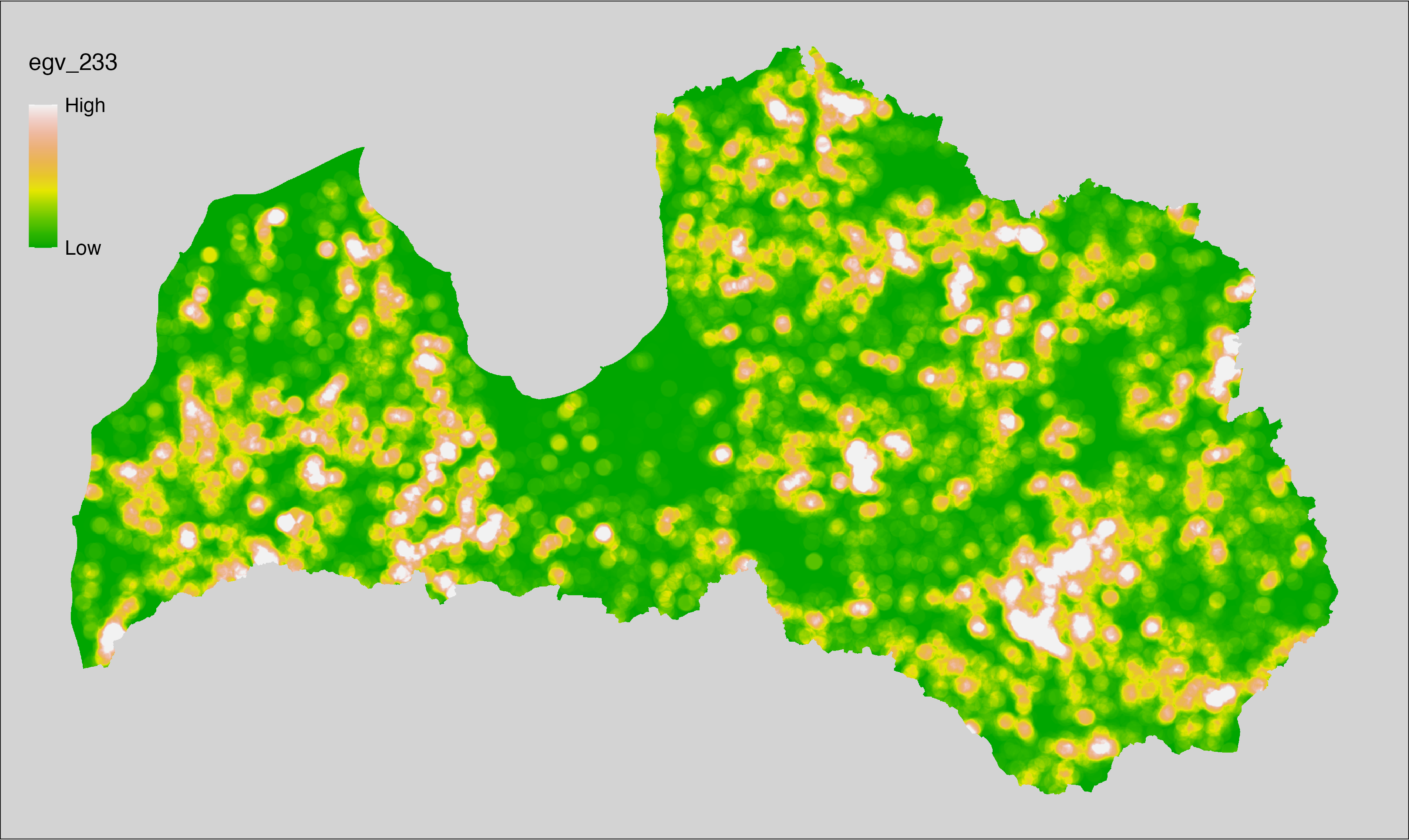
6.234 FarmlandGrassland_GrasslandsTemporary_r10000
filename: FarmlandGrassland_GrasslandsTemporary_r10000.tif
layername: egv_234
English name: Fractional cover of Temporary Grassland within the 10 km landscape
Latvian name: Zālāju-aramzemē platības īpatsvars 10 km ainavā
Procedure: The cover fraction within a radius of 10000 m around the analysis grid cell
is calculated as the area-weighted sum of the analysis cells inside
the buffer, using the workflow egvtools::radius_function(). During the calculation of the landscape
metric, inverse distance weighted (power = 2) gap filling on the output is
applied to ensure no missing values at the edges. Then the layer is
rewritten to set its name. Finally, the layer is standardised by
subtracting the arithmetic mean and dividing by the root mean squared error.
Code
# libs ----
if(!require(terra)) {install.packages("terra"); require(terra)}
if(!require(egvtools)) {remotes::install_github("aavotins/egvtools"); require(egvtools)}
# Templates -----
template100=rast("./Templates/TemplateRasters/LV100m_10km.tif")
# radii ----
radius_function(
kvadrati_path = "./Templates/TemplateGrids/tiles/",
radii_path = "./Templates/TemplateGridPoints/tiles/",
tikls100_path = "./Templates/TemplateGrids/tikls100_sauzeme.parquet",
template_path = "./Templates/TemplateRasters/LV100m_10km.tif",
input_layers = c("./RasterGrids_100m/2024/RAW/FarmlandGrassland_GrasslandsTemporary_cell.tif"),
layer_prefixes = c("FarmlandGrassland_GrasslandsTemporary"),
output_dir = "./RasterGrids_100m/2024/RAW/",
n_workers = 6,
radii = c("r10000"),
radius_mode = "sparse",
extract_fun = "mean",
fill_missing = TRUE,
IDW_weight = 2,
future_max_size = 40 * 1024^3)
# FarmlandGrassland_GrasslandsTemporary_r10000.tif egv_234
slanis=rast("./RasterGrids_100m/2024/RAW/FarmlandGrassland_GrasslandsTemporary_r10000.tif")
names(slanis)="egv_234"
slanis2=project(slanis,template100)
writeRaster(slanis2,
"./RasterGrids_100m/2024/RAW/FarmlandGrassland_GrasslandsTemporary_r10000.tif",
overwrite=TRUE)
# standardisation ----
if(!require(terra)) {install.packages("terra"); require(terra)}
if(!require(tidyverse)) {install.packages("tidyverse"); require(tidyverse)}
nosaukums="FarmlandGrassland_GrasslandsTemporary_r10000.tif"
ielasisanas_cels=paste0("./RasterGrids_100m/2024/RAW/",nosaukums)
saglabasanas_cels=paste0("./RasterGrids_100m/2024/Scaled/",nosaukums)
slanis=rast(ielasisanas_cels)
videjais=global(slanis,fun="mean",na.rm=TRUE)
centrets=slanis-videjais[,1]
standartnovirze=terra::global(centrets,fun="rms",na.rm=TRUE)
merogots=centrets/standartnovirze[,1]
writeRaster(merogots,
filename=saglabasanas_cels,
overwrite=TRUE)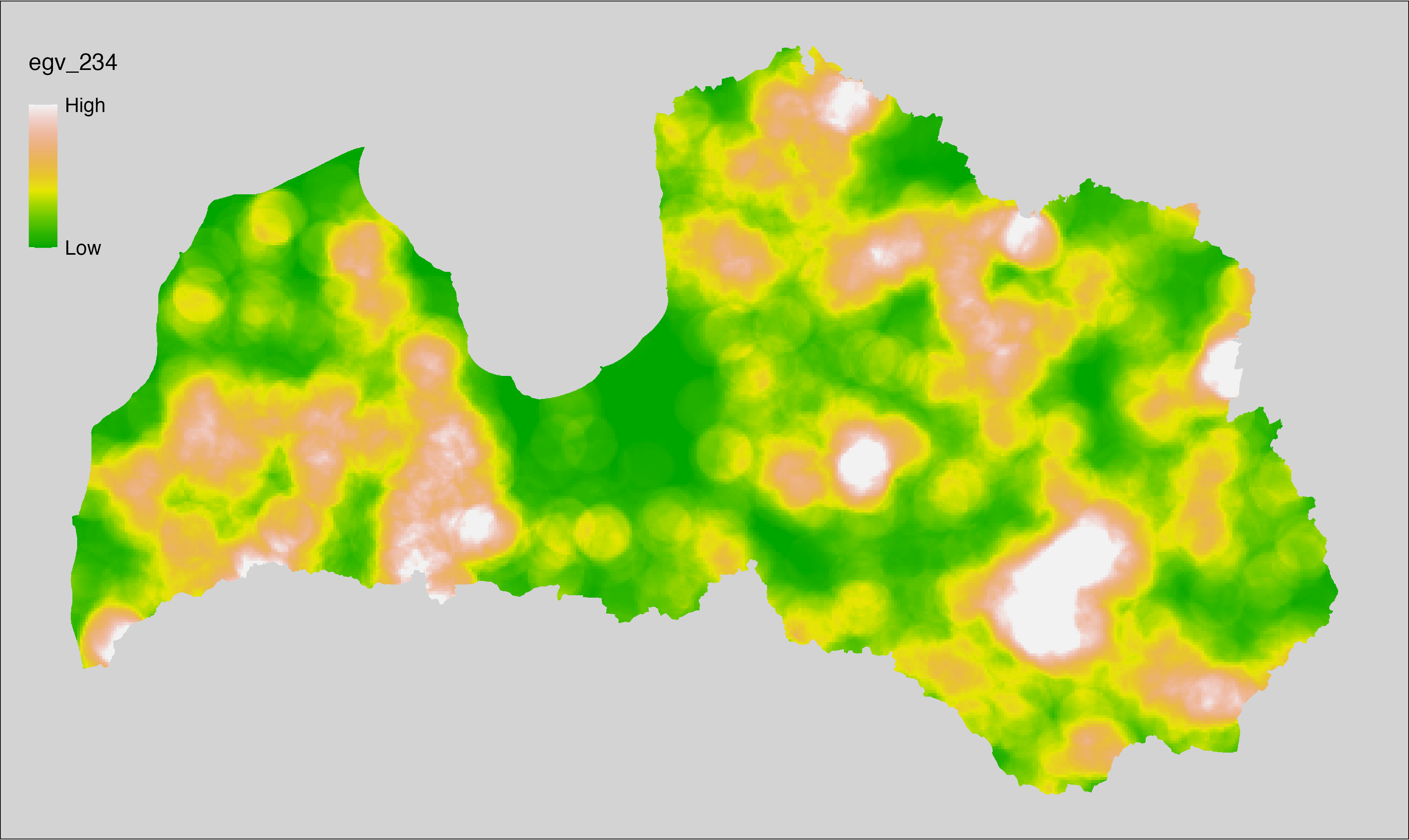
6.235 FarmlandParcels_FieldsActive_cell
filename: FarmlandParcels_FieldsActive_cell.tif
layername: egv_235
English name: Fractional cover of Agricultural Land Parcels within the analysis cell (1 ha)
Latvian name: Lauku bloku platības īpatsvars analīzes šūnā (1 ha)
Procedure: First, agricultural parcels from the Rural Support Service’s
information on declared fields are rasterised to input resolution,
ensuring value 1 at the polygon locations and value 0 elsewhere. Rasterisation
is performed with the workflow egvtools::polygon2input(). Once rasterised, the layer is
aggregated to EGV resolution using the workflow egvtools::input2egv(), which
calculates the arithmetic mean and thus results in a cover fraction. During aggregation, inverse
distance weighted (power = 2) gap filling on the output is applied to
ensure no missing values at the edges. Finally, the layer is standardised
by subtracting the arithmetic mean and dividing by the root mean squared error.
Code
# libs ----
if(!require(egvtools)) {remotes::install_github("aavotins/egvtools"); require(egvtools)}
if(!require(terra)) {install.packages("terra"); require(terra)}
if(!require(sf)) {install.packages("sf"); require(sf)}
if(!require(tidyverse)) {install.packages("tidyverse"); require(tidyverse)}
if(!require(sfarrow)) {install.packages("sfarrow"); require(sfarrow)}
if(!require(readxl)) {install.packages("readxl"); require(readxl)}
if(!require(raster)) {install.packages("raster"); require(raster)}
if(!require(fasterize)) {install.packages("fasterize"); require(fasterize)}
# templates ----
template100=rast("./Templates/TemplateRasters/LV100m_10km.tif")
template10=rast("./Templates/TemplateRasters/LV10m_10km.tif")
rastrs10=raster(template10)
nulls10=rast("./Templates/TemplateRasters/nulls_LV10m_10km.tif")
nulls100=rast("./Templates/TemplateRasters/nulls_LV100m_10km.tif")
# codes ----
kodi=read_excel("./Geodata/2024/LAD/KulturuKodi_2024.xlsx")
kodi$kods=as.character(kodi$kods)
# LAD ----
lad=sfarrow::st_read_parquet("./Geodata/2024/LAD/Lauki_2024.parquet")
lad$yes=1
lad=lad %>%
left_join(kodi,by=c("PRODUCT_CODE"="kods"))
# simple landscape ----
simple_landscape=rast("RasterGrids_10m/2024/Ainava_vienk_mask.tif")
# FarmlandParcels_FieldsActive_cell.tif egv_235 ----
p2i_rez=egvtools::polygon2input(vector_data = lad,
template_path = "./Templates/TemplateRasters/LV10m_10km.tif",
out_path = "./RasterGrids_10m/2024/",
file_name = "FarmlandParcels_FieldsActive_input.tif",
value_field = "yes",
prepare=FALSE,
background_raster = "./Templates/TemplateRasters/nulls_LV10m_10km.tif",
plot_result = TRUE)
p2i_rez
i2e_rez=egvtools::input2egv(input=paste0("./RasterGrids_10m/2024/",
"FarmlandParcels_FieldsActive_input.tif"),
egv_template= "./Templates/TemplateRasters/LV100m_10km.tif",
summary_function = "average",
missing_job = "FillOutput",
outlocation = "./RasterGrids_100m/2024/RAW/",
outfilename = "FarmlandParcels_FieldsActive_cell.tif",
layername = "egv_235",
idw_weight = 2,
plot_gaps = FALSE,plot_final = TRUE)
i2e_rez
rm(p2i_rez)
rm(i2e_rez)
rm(dati)
unlink("./RasterGrids_10m/2024/FarmlandParcels_FieldsActive_input.tif")
# standardisation ----
if(!require(terra)) {install.packages("terra"); require(terra)}
if(!require(tidyverse)) {install.packages("tidyverse"); require(tidyverse)}
nosaukums="FarmlandParcels_FieldsActive_cell.tif"
ielasisanas_cels=paste0("./RasterGrids_100m/2024/RAW/",nosaukums)
saglabasanas_cels=paste0("./RasterGrids_100m/2024/Scaled/",nosaukums)
slanis=rast(ielasisanas_cels)
videjais=global(slanis,fun="mean",na.rm=TRUE)
centrets=slanis-videjais[,1]
standartnovirze=terra::global(centrets,fun="rms",na.rm=TRUE)
merogots=centrets/standartnovirze[,1]
writeRaster(merogots,
filename=saglabasanas_cels,
overwrite=TRUE)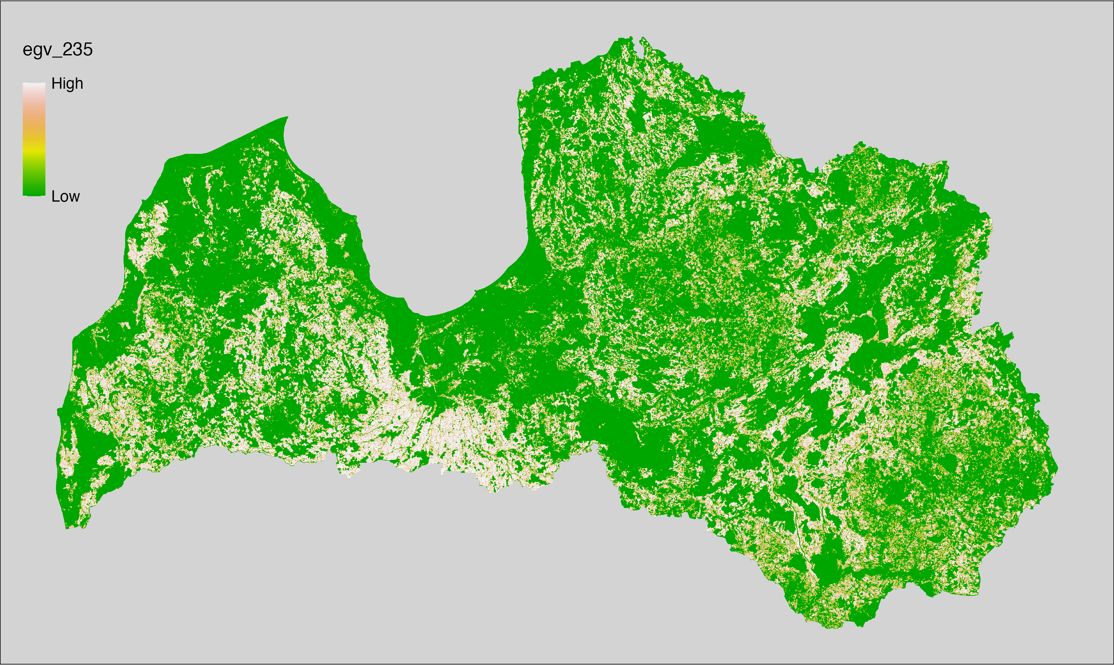
6.236 FarmlandParcels_FieldsActive_r500
filename: FarmlandParcels_FieldsActive_r500.tif
layername: egv_236
English name: Fractional cover of Agricultural Land Parcels within the 0.5 km landscape
Latvian name: Lauku bloku platības īpatsvars 0,5 km ainavā
Procedure: The cover fraction within a radius of 500 m around the analysis grid cell is
calculated as the area-weighted sum of the analysis cells inside the
buffer, using the workflow egvtools::radius_function(). During the calculation of the landscape metric,
inverse distance weighted (power = 2) gap filling on the output is applied
to ensure no missing values at the edges. Then the layer is rewritten to set
its name. Finally, the layer is standardised by subtracting the arithmetic
mean and dividing by the root mean squared error.
Code
# libs ----
if(!require(terra)) {install.packages("terra"); require(terra)}
if(!require(egvtools)) {remotes::install_github("aavotins/egvtools"); require(egvtools)}
# Templates -----
template100=rast("./Templates/TemplateRasters/LV100m_10km.tif")
# radii ----
radius_function(
kvadrati_path = "./Templates/TemplateGrids/tiles/",
radii_path = "./Templates/TemplateGridPoints/tiles/",
tikls100_path = "./Templates/TemplateGrids/tikls100_sauzeme.parquet",
template_path = "./Templates/TemplateRasters/LV100m_10km.tif",
input_layers = c("./RasterGrids_100m/2024/RAW/FarmlandParcels_FieldsActive_cell.tif"),
layer_prefixes = c("FarmlandParcels_FieldsActive"),
output_dir = "./RasterGrids_100m/2024/RAW/",
n_workers = 6,
radii = c("r500"),
radius_mode = "sparse",
extract_fun = "mean",
fill_missing = TRUE,
IDW_weight = 2,
future_max_size = 40 * 1024^3)
# FarmlandParcels_FieldsActive_r500.tif egv_236
slanis=rast("./RasterGrids_100m/2024/RAW/FarmlandParcels_FieldsActive_r500.tif")
names(slanis)="egv_236"
slanis2=project(slanis,template100)
writeRaster(slanis2,
"./RasterGrids_100m/2024/RAW/FarmlandParcels_FieldsActive_r500.tif",
overwrite=TRUE)
# standardisation ----
if(!require(terra)) {install.packages("terra"); require(terra)}
if(!require(tidyverse)) {install.packages("tidyverse"); require(tidyverse)}
nosaukums="FarmlandParcels_FieldsActive_r500.tif"
ielasisanas_cels=paste0("./RasterGrids_100m/2024/RAW/",nosaukums)
saglabasanas_cels=paste0("./RasterGrids_100m/2024/Scaled/",nosaukums)
slanis=rast(ielasisanas_cels)
videjais=global(slanis,fun="mean",na.rm=TRUE)
centrets=slanis-videjais[,1]
standartnovirze=terra::global(centrets,fun="rms",na.rm=TRUE)
merogots=centrets/standartnovirze[,1]
writeRaster(merogots,
filename=saglabasanas_cels,
overwrite=TRUE)
6.237 FarmlandParcels_FieldsActive_r1250
filename: FarmlandParcels_FieldsActive_r1250.tif
layername: egv_237
English name: Fractional cover of Agricultural Land Parcels within the 1.25 km landscape
Latvian name: Lauku bloku platības īpatsvars 1,25 km ainavā
Procedure: The cover fraction within a radius of 1250 m around the analysis grid cell
is calculated as the area-weighted sum of the analysis cells inside
the buffer, using the workflow egvtools::radius_function(). During the calculation of the landscape
metric, inverse distance weighted (power = 2) gap filling on the output is
applied to ensure no missing values at the edges. Then the layer is
rewritten to set its name. Finally, the layer is standardised by
subtracting the arithmetic mean and dividing by the root mean squared error.
Code
# libs ----
if(!require(terra)) {install.packages("terra"); require(terra)}
if(!require(egvtools)) {remotes::install_github("aavotins/egvtools"); require(egvtools)}
# Templates -----
template100=rast("./Templates/TemplateRasters/LV100m_10km.tif")
# radii ----
radius_function(
kvadrati_path = "./Templates/TemplateGrids/tiles/",
radii_path = "./Templates/TemplateGridPoints/tiles/",
tikls100_path = "./Templates/TemplateGrids/tikls100_sauzeme.parquet",
template_path = "./Templates/TemplateRasters/LV100m_10km.tif",
input_layers = c("./RasterGrids_100m/2024/RAW/FarmlandParcels_FieldsActive_cell.tif"),
layer_prefixes = c("FarmlandParcels_FieldsActive"),
output_dir = "./RasterGrids_100m/2024/RAW/",
n_workers = 6,
radii = c("r1250"),
radius_mode = "sparse",
extract_fun = "mean",
fill_missing = TRUE,
IDW_weight = 2,
future_max_size = 40 * 1024^3)
# FarmlandParcels_FieldsActive_r1250.tif egv_237
slanis=rast("./RasterGrids_100m/2024/RAW/FarmlandParcels_FieldsActive_r1250.tif")
names(slanis)="egv_237"
slanis2=project(slanis,template100)
writeRaster(slanis2,
"./RasterGrids_100m/2024/RAW/FarmlandParcels_FieldsActive_r1250.tif",
overwrite=TRUE)
# standardisation ----
if(!require(terra)) {install.packages("terra"); require(terra)}
if(!require(tidyverse)) {install.packages("tidyverse"); require(tidyverse)}
nosaukums="FarmlandParcels_FieldsActive_r1250.tif"
ielasisanas_cels=paste0("./RasterGrids_100m/2024/RAW/",nosaukums)
saglabasanas_cels=paste0("./RasterGrids_100m/2024/Scaled/",nosaukums)
slanis=rast(ielasisanas_cels)
videjais=global(slanis,fun="mean",na.rm=TRUE)
centrets=slanis-videjais[,1]
standartnovirze=terra::global(centrets,fun="rms",na.rm=TRUE)
merogots=centrets/standartnovirze[,1]
writeRaster(merogots,
filename=saglabasanas_cels,
overwrite=TRUE)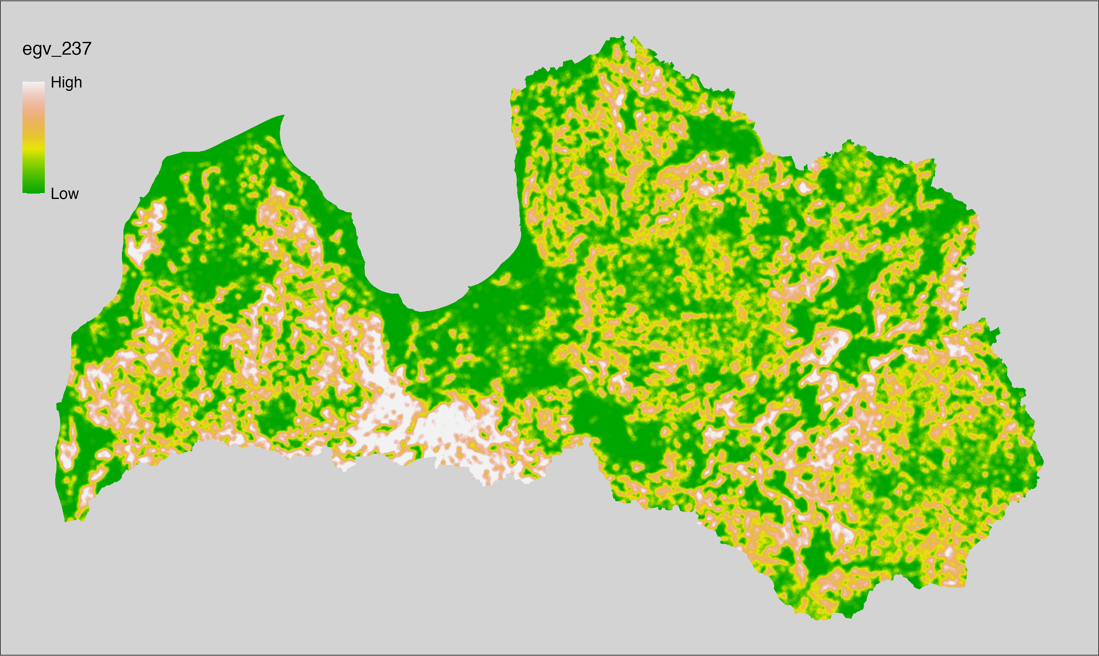
6.238 FarmlandParcels_FieldsActive_r3000
filename: FarmlandParcels_FieldsActive_r3000.tif
layername: egv_238
English name: Fractional cover of Agricultural Land Parcels within the 3 km landscape
Latvian name: Lauku bloku platības īpatsvars 3 km ainavā
Procedure: The cover fraction within a radius of 3000 m around the analysis grid cell
is calculated as the area-weighted sum of the analysis cells inside
the buffer, using the workflow egvtools::radius_function(). During the calculation of the landscape
metric, inverse distance weighted (power = 2) gap filling on the output is
applied to ensure no missing values at the edges. Then the layer is
rewritten to set its name. Finally, the layer is standardised by
subtracting the arithmetic mean and dividing by the root mean squared error.
Code
# libs ----
if(!require(terra)) {install.packages("terra"); require(terra)}
if(!require(egvtools)) {remotes::install_github("aavotins/egvtools"); require(egvtools)}
# Templates -----
template100=rast("./Templates/TemplateRasters/LV100m_10km.tif")
# radii ----
radius_function(
kvadrati_path = "./Templates/TemplateGrids/tiles/",
radii_path = "./Templates/TemplateGridPoints/tiles/",
tikls100_path = "./Templates/TemplateGrids/tikls100_sauzeme.parquet",
template_path = "./Templates/TemplateRasters/LV100m_10km.tif",
input_layers = c("./RasterGrids_100m/2024/RAW/FarmlandParcels_FieldsActive_cell.tif"),
layer_prefixes = c("FarmlandParcels_FieldsActive"),
output_dir = "./RasterGrids_100m/2024/RAW/",
n_workers = 6,
radii = c("r3000"),
radius_mode = "sparse",
extract_fun = "mean",
fill_missing = TRUE,
IDW_weight = 2,
future_max_size = 40 * 1024^3)
# FarmlandParcels_FieldsActive_r3000.tif egv_238
slanis=rast("./RasterGrids_100m/2024/RAW/FarmlandParcels_FieldsActive_r3000.tif")
names(slanis)="egv_238"
slanis2=project(slanis,template100)
writeRaster(slanis2,
"./RasterGrids_100m/2024/RAW/FarmlandParcels_FieldsActive_r3000.tif",
overwrite=TRUE)
# standardisation ----
if(!require(terra)) {install.packages("terra"); require(terra)}
if(!require(tidyverse)) {install.packages("tidyverse"); require(tidyverse)}
nosaukums="FarmlandParcels_FieldsActive_r3000.tif"
ielasisanas_cels=paste0("./RasterGrids_100m/2024/RAW/",nosaukums)
saglabasanas_cels=paste0("./RasterGrids_100m/2024/Scaled/",nosaukums)
slanis=rast(ielasisanas_cels)
videjais=global(slanis,fun="mean",na.rm=TRUE)
centrets=slanis-videjais[,1]
standartnovirze=terra::global(centrets,fun="rms",na.rm=TRUE)
merogots=centrets/standartnovirze[,1]
writeRaster(merogots,
filename=saglabasanas_cels,
overwrite=TRUE)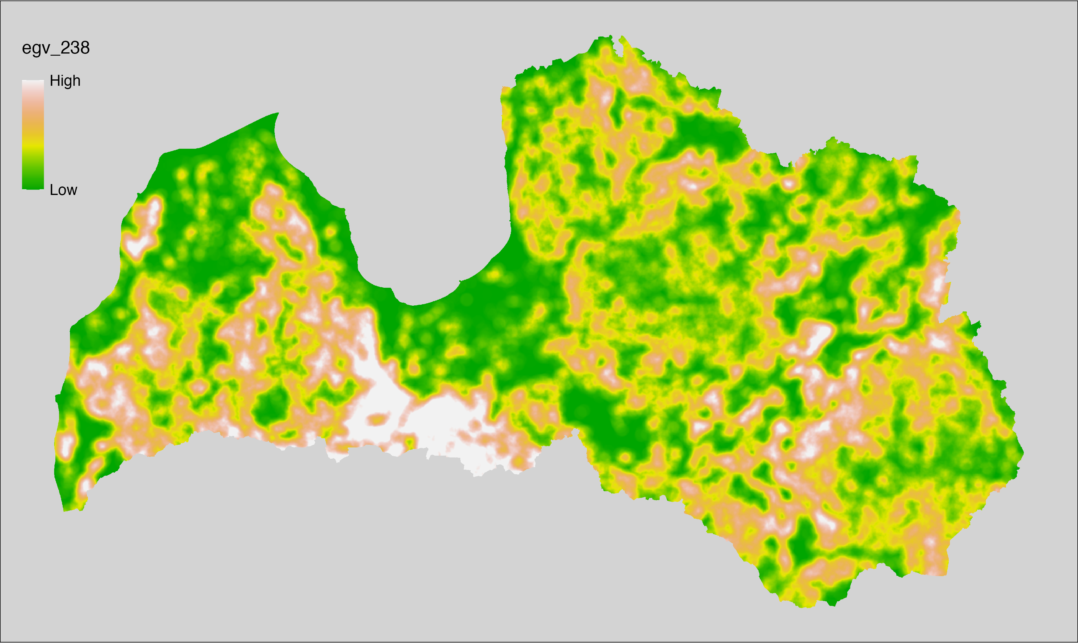
6.239 FarmlandParcels_FieldsActive_r10000
filename: FarmlandParcels_FieldsActive_r10000.tif
layername: egv_239
English name: Fractional cover of Agricultural Land Parcels within the 10 km landscape
Latvian name: Lauku bloku platības īpatsvars 10 km ainavā
Procedure: The cover fraction within a radius of 10000 m around the analysis grid cell
is calculated as the area-weighted sum of the analysis cells inside
the buffer, using the workflow egvtools::radius_function(). During the calculation of the landscape
metric, inverse distance weighted (power = 2) gap filling on the output is
applied to ensure no missing values at the edges. Then the layer is
rewritten to set its name. Finally, the layer is standardised by
subtracting the arithmetic mean and dividing by the root mean squared error.
Code
# libs ----
if(!require(terra)) {install.packages("terra"); require(terra)}
if(!require(egvtools)) {remotes::install_github("aavotins/egvtools"); require(egvtools)}
# Templates -----
template100=rast("./Templates/TemplateRasters/LV100m_10km.tif")
# radii ----
radius_function(
kvadrati_path = "./Templates/TemplateGrids/tiles/",
radii_path = "./Templates/TemplateGridPoints/tiles/",
tikls100_path = "./Templates/TemplateGrids/tikls100_sauzeme.parquet",
template_path = "./Templates/TemplateRasters/LV100m_10km.tif",
input_layers = c("./RasterGrids_100m/2024/RAW/FarmlandParcels_FieldsActive_cell.tif"),
layer_prefixes = c("FarmlandParcels_FieldsActive"),
output_dir = "./RasterGrids_100m/2024/RAW/",
n_workers = 6,
radii = c("r10000"),
radius_mode = "sparse",
extract_fun = "mean",
fill_missing = TRUE,
IDW_weight = 2,
future_max_size = 40 * 1024^3)
# FarmlandParcels_FieldsActive_r10000.tif egv_239
slanis=rast("./RasterGrids_100m/2024/RAW/FarmlandParcels_FieldsActive_r10000.tif")
names(slanis)="egv_239"
slanis2=project(slanis,template100)
writeRaster(slanis2,
"./RasterGrids_100m/2024/RAW/FarmlandParcels_FieldsActive_r10000.tif",
overwrite=TRUE)
# standardisation ----
if(!require(terra)) {install.packages("terra"); require(terra)}
if(!require(tidyverse)) {install.packages("tidyverse"); require(tidyverse)}
nosaukums="FarmlandParcels_FieldsActive_r10000.tif"
ielasisanas_cels=paste0("./RasterGrids_100m/2024/RAW/",nosaukums)
saglabasanas_cels=paste0("./RasterGrids_100m/2024/Scaled/",nosaukums)
slanis=rast(ielasisanas_cels)
videjais=global(slanis,fun="mean",na.rm=TRUE)
centrets=slanis-videjais[,1]
standartnovirze=terra::global(centrets,fun="rms",na.rm=TRUE)
merogots=centrets/standartnovirze[,1]
writeRaster(merogots,
filename=saglabasanas_cels,
overwrite=TRUE)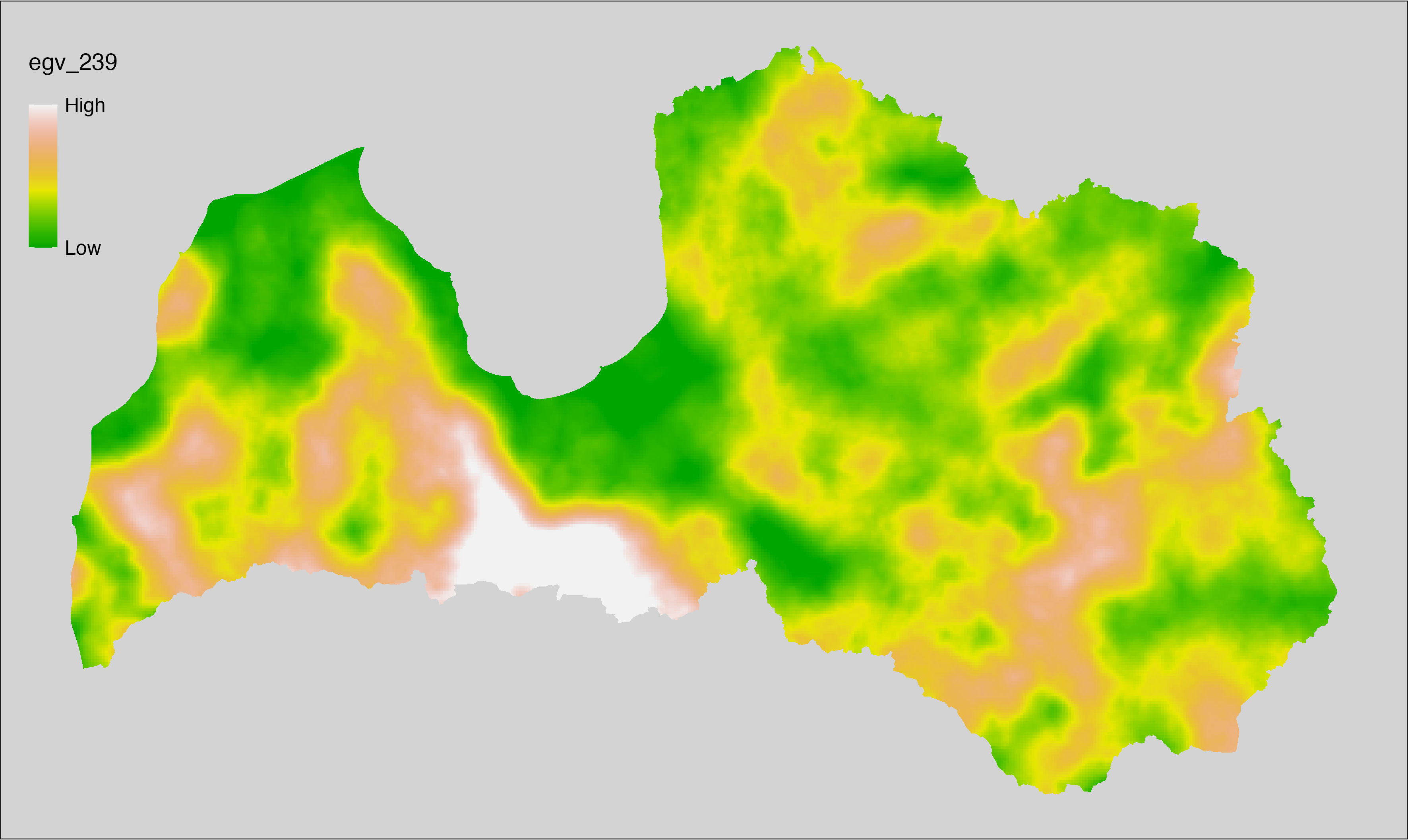
6.240 FarmlandPloughed_CropsFallow_cell
filename: FarmlandPloughed_CropsFallow_cell.tif
layername: egv_240
English name: Fractional cover of Crop-, Fallow- Land within the analysis cell (1 ha)
Latvian name: Aramzemju, papuvju platības īpatsvars analīzes šūnā (1 ha)
Procedure: First, agricultural parcels declared as crops or fallow land are
selected from the Rural Support Service’s information on declared
fields. Geometries are then rasterised to input resolution, ensuring
value 1 at the polygon locations and value 0 elsewhere. Rasterisation is
performed using the workflow egvtools::polygon2input(). Once rasterised, the
layer is aggregated to EGV resolution using the workflow egvtools::input2egv(),
which calculates the arithmetic mean and thus
results in a cover fraction. During aggregation, inverse
distance weighted (power = 2) gap filling on the output is applied to
ensure no missing values at the edges. Finally, the layer is standardised
by subtracting the arithmetic mean and dividing by the root mean squared error.
Code
# libs ----
if(!require(egvtools)) {remotes::install_github("aavotins/egvtools"); require(egvtools)}
if(!require(terra)) {install.packages("terra"); require(terra)}
if(!require(sf)) {install.packages("sf"); require(sf)}
if(!require(tidyverse)) {install.packages("tidyverse"); require(tidyverse)}
if(!require(sfarrow)) {install.packages("sfarrow"); require(sfarrow)}
if(!require(readxl)) {install.packages("readxl"); require(readxl)}
if(!require(raster)) {install.packages("raster"); require(raster)}
if(!require(fasterize)) {install.packages("fasterize"); require(fasterize)}
# templates ----
template100=rast("./Templates/TemplateRasters/LV100m_10km.tif")
template10=rast("./Templates/TemplateRasters/LV10m_10km.tif")
rastrs10=raster(template10)
nulls10=rast("./Templates/TemplateRasters/nulls_LV10m_10km.tif")
nulls100=rast("./Templates/TemplateRasters/nulls_LV100m_10km.tif")
# codes ----
kodi=read_excel("./Geodata/2024/LAD/KulturuKodi_2024.xlsx")
kodi$kods=as.character(kodi$kods)
# LAD ----
lad=sfarrow::st_read_parquet("./Geodata/2024/LAD/Lauki_2024.parquet")
lad$yes=1
lad=lad %>%
left_join(kodi,by=c("PRODUCT_CODE"="kods"))
# simple landscape ----
simple_landscape=rast("RasterGrids_10m/2024/Ainava_vienk_mask.tif")
# FarmlandPloughed_CropsFallow_cell.tif egv_240 ----
dati=lad %>%
filter(SDM_grupa_sakums %in% c("aramzemes (citur neiekļautās)",
"aramzemes (labība-vasarāji)",
"aramzemes (labība-ziemāji)",
"aramzemes (vagu un rušināmkultūru)",
"aramzemes (vasaras rapsis un rispsis, kukurūzas, zirņi un pupas, soja, kaņepes)",
"aramzemes (ziemas rapsis un ripsis)",
"papuves"))
table(dati$SDM_grupa_sakums,useNA="always")
p2i_rez=egvtools::polygon2input(vector_data = dati,
template_path = "./Templates/TemplateRasters/LV10m_10km.tif",
out_path = "./RasterGrids_10m/2024/",
file_name = "FarmlandPloughed_CropsFallow_input.tif",
value_field = "yes",
prepare=FALSE,
background_raster = "./Templates/TemplateRasters/nulls_LV10m_10km.tif",
plot_result = TRUE)
p2i_rez
i2e_rez=egvtools::input2egv(input=paste0("./RasterGrids_10m/2024/",
"FarmlandPloughed_CropsFallow_input.tif"),
egv_template= "./Templates/TemplateRasters/LV100m_10km.tif",
summary_function = "average",
missing_job = "FillOutput",
outlocation = "./RasterGrids_100m/2024/RAW/",
outfilename = "FarmlandPloughed_CropsFallow_cell.tif",
layername = "egv_240",
idw_weight = 2,
plot_gaps = FALSE,plot_final = TRUE)
i2e_rez
rm(p2i_rez)
rm(i2e_rez)
rm(dati)
unlink("./RasterGrids_10m/2024/FarmlandPloughed_CropsFallow_input.tif")
# standardisation ----
if(!require(terra)) {install.packages("terra"); require(terra)}
if(!require(tidyverse)) {install.packages("tidyverse"); require(tidyverse)}
nosaukums="FarmlandPloughed_CropsFallow_cell.tif"
ielasisanas_cels=paste0("./RasterGrids_100m/2024/RAW/",nosaukums)
saglabasanas_cels=paste0("./RasterGrids_100m/2024/Scaled/",nosaukums)
slanis=rast(ielasisanas_cels)
videjais=global(slanis,fun="mean",na.rm=TRUE)
centrets=slanis-videjais[,1]
standartnovirze=terra::global(centrets,fun="rms",na.rm=TRUE)
merogots=centrets/standartnovirze[,1]
writeRaster(merogots,
filename=saglabasanas_cels,
overwrite=TRUE)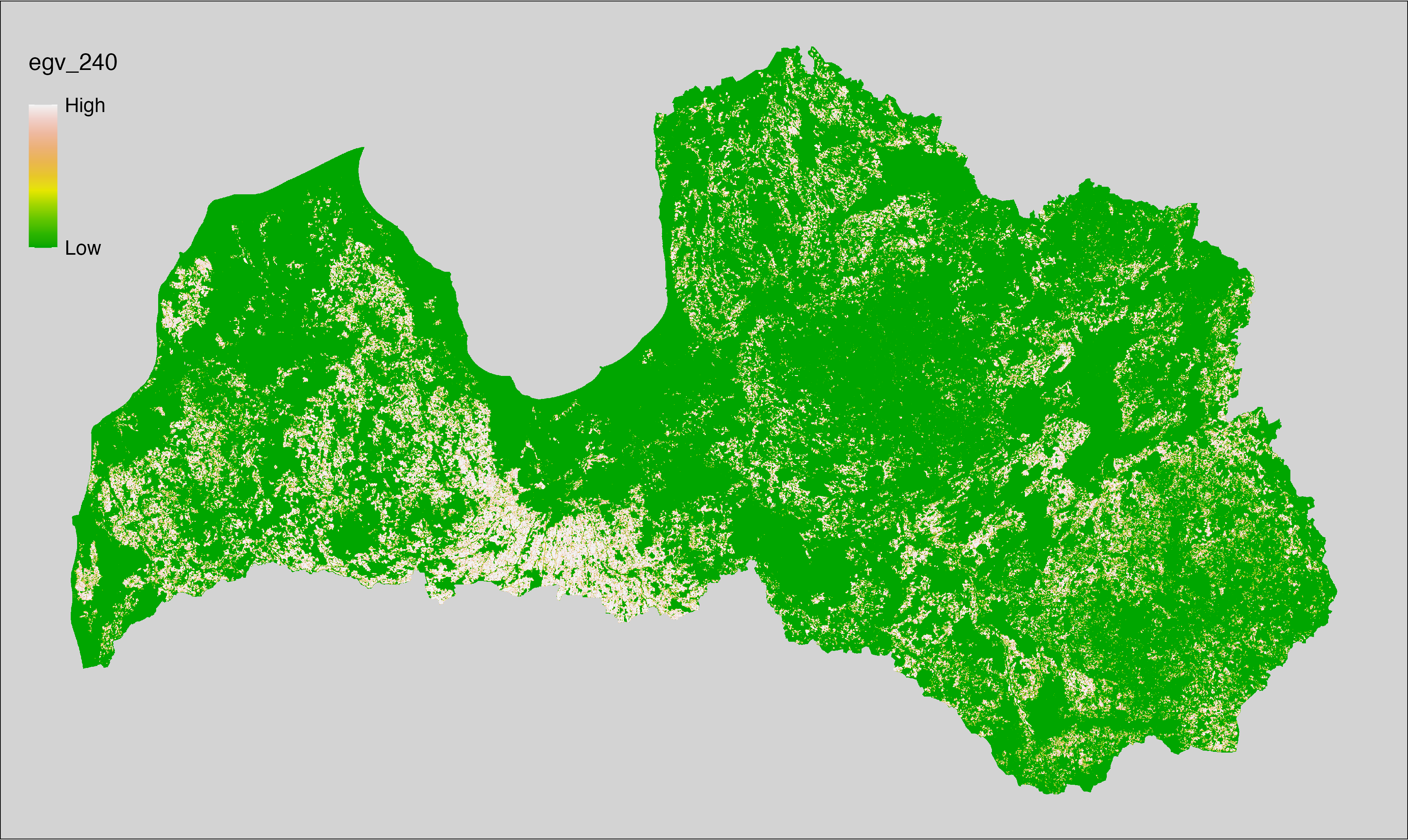
6.241 FarmlandPloughed_CropsFallow_r500
filename: FarmlandPloughed_CropsFallow_r500.tif
layername: egv_241
English name: Fractional cover of Crop-, Fallow- Land within the 0.5 km landscape
Latvian name: Aramzemju, papuvju platības īpatsvars 0,5 km ainavā
Procedure: The cover fraction within a radius of 500 m around the analysis grid cell is
calculated as the area-weighted sum of the analysis cells inside the
buffer, using the workflow egvtools::radius_function(). During the calculation of the landscape metric,
inverse distance weighted (power = 2) gap filling on the output is applied
to ensure no missing values at the edges. Then the layer is rewritten to set
its name. Finally, the layer is standardised by subtracting the arithmetic
mean and dividing by the root mean squared error.
Code
# libs ----
if(!require(terra)) {install.packages("terra"); require(terra)}
if(!require(egvtools)) {remotes::install_github("aavotins/egvtools"); require(egvtools)}
# Templates -----
template100=rast("./Templates/TemplateRasters/LV100m_10km.tif")
# radii ----
radius_function(
kvadrati_path = "./Templates/TemplateGrids/tiles/",
radii_path = "./Templates/TemplateGridPoints/tiles/",
tikls100_path = "./Templates/TemplateGrids/tikls100_sauzeme.parquet",
template_path = "./Templates/TemplateRasters/LV100m_10km.tif",
input_layers = c("./RasterGrids_100m/2024/RAW/FarmlandPloughed_CropsFallow_cell.tif"),
layer_prefixes = c("FarmlandPloughed_CropsFallow"),
output_dir = "./RasterGrids_100m/2024/RAW/",
n_workers = 6,
radii = c("r500"),
radius_mode = "sparse",
extract_fun = "mean",
fill_missing = TRUE,
IDW_weight = 2,
future_max_size = 40 * 1024^3)
# FarmlandPloughed_CropsFallow_r500.tif egv_241
slanis=rast("./RasterGrids_100m/2024/RAW/FarmlandPloughed_CropsFallow_r500.tif")
names(slanis)="egv_241"
slanis2=project(slanis,template100)
writeRaster(slanis2,
"./RasterGrids_100m/2024/RAW/FarmlandPloughed_CropsFallow_r500.tif",
overwrite=TRUE)
# standardisation ----
if(!require(terra)) {install.packages("terra"); require(terra)}
if(!require(tidyverse)) {install.packages("tidyverse"); require(tidyverse)}
nosaukums="FarmlandPloughed_CropsFallow_r500.tif"
ielasisanas_cels=paste0("./RasterGrids_100m/2024/RAW/",nosaukums)
saglabasanas_cels=paste0("./RasterGrids_100m/2024/Scaled/",nosaukums)
slanis=rast(ielasisanas_cels)
videjais=global(slanis,fun="mean",na.rm=TRUE)
centrets=slanis-videjais[,1]
standartnovirze=terra::global(centrets,fun="rms",na.rm=TRUE)
merogots=centrets/standartnovirze[,1]
writeRaster(merogots,
filename=saglabasanas_cels,
overwrite=TRUE)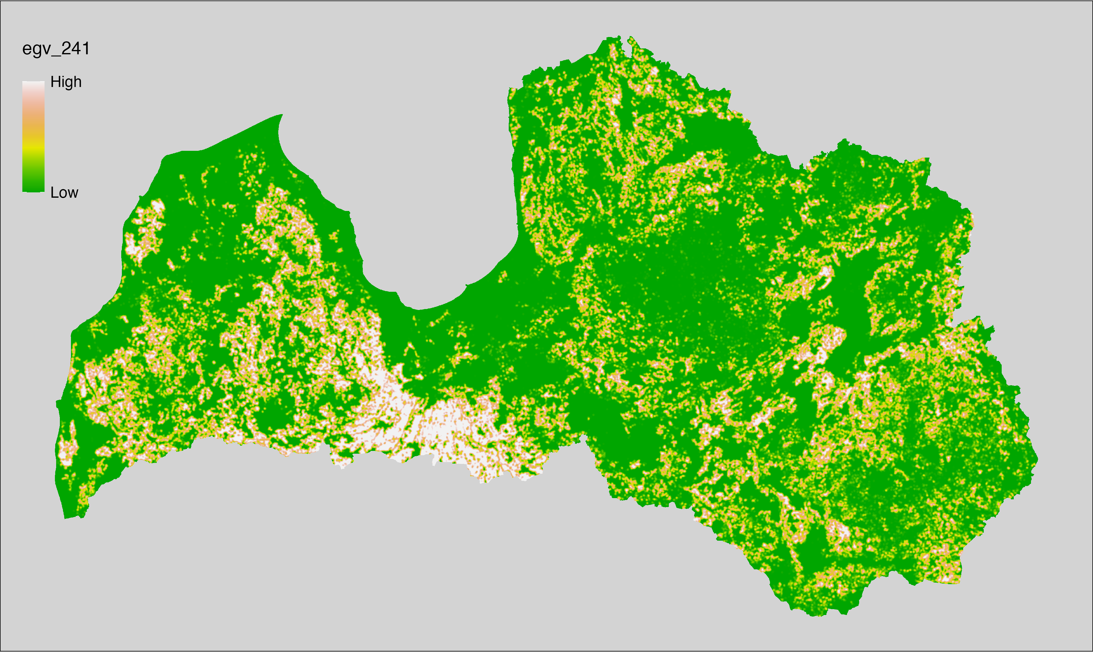
6.242 FarmlandPloughed_CropsFallow_r1250
filename: FarmlandPloughed_CropsFallow_r1250.tif
layername: egv_242
English name: Fractional cover of Crop-, Fallow- Land within the 1.25 km landscape
Latvian name: Aramzemju, papuvju platības īpatsvars 1,25 km ainavā
Procedure: The cover fraction within a radius of 1250 m around the analysis grid cell
is calculated as the area-weighted sum of the analysis cells inside
the buffer, using the workflow egvtools::radius_function(). During the calculation of the landscape
metric, inverse distance weighted (power = 2) gap filling on the output is
applied to ensure no missing values at the edges. Then the layer is
rewritten to set its name. Finally, the layer is standardised by
subtracting the arithmetic mean and dividing by the root mean squared error.
Code
# libs ----
if(!require(terra)) {install.packages("terra"); require(terra)}
if(!require(egvtools)) {remotes::install_github("aavotins/egvtools"); require(egvtools)}
# Templates -----
template100=rast("./Templates/TemplateRasters/LV100m_10km.tif")
# radii ----
radius_function(
kvadrati_path = "./Templates/TemplateGrids/tiles/",
radii_path = "./Templates/TemplateGridPoints/tiles/",
tikls100_path = "./Templates/TemplateGrids/tikls100_sauzeme.parquet",
template_path = "./Templates/TemplateRasters/LV100m_10km.tif",
input_layers = c("./RasterGrids_100m/2024/RAW/FarmlandPloughed_CropsFallow_cell.tif"),
layer_prefixes = c("FarmlandPloughed_CropsFallow"),
output_dir = "./RasterGrids_100m/2024/RAW/",
n_workers = 6,
radii = c("r1250"),
radius_mode = "sparse",
extract_fun = "mean",
fill_missing = TRUE,
IDW_weight = 2,
future_max_size = 40 * 1024^3)
# FarmlandPloughed_CropsFallow_r1250.tif egv_242
slanis=rast("./RasterGrids_100m/2024/RAW/FarmlandPloughed_CropsFallow_r1250.tif")
names(slanis)="egv_242"
slanis2=project(slanis,template100)
writeRaster(slanis2,
"./RasterGrids_100m/2024/RAW/FarmlandPloughed_CropsFallow_r1250.tif",
overwrite=TRUE)
# standardisation ----
if(!require(terra)) {install.packages("terra"); require(terra)}
if(!require(tidyverse)) {install.packages("tidyverse"); require(tidyverse)}
nosaukums="FarmlandPloughed_CropsFallow_r1250.tif"
ielasisanas_cels=paste0("./RasterGrids_100m/2024/RAW/",nosaukums)
saglabasanas_cels=paste0("./RasterGrids_100m/2024/Scaled/",nosaukums)
slanis=rast(ielasisanas_cels)
videjais=global(slanis,fun="mean",na.rm=TRUE)
centrets=slanis-videjais[,1]
standartnovirze=terra::global(centrets,fun="rms",na.rm=TRUE)
merogots=centrets/standartnovirze[,1]
writeRaster(merogots,
filename=saglabasanas_cels,
overwrite=TRUE)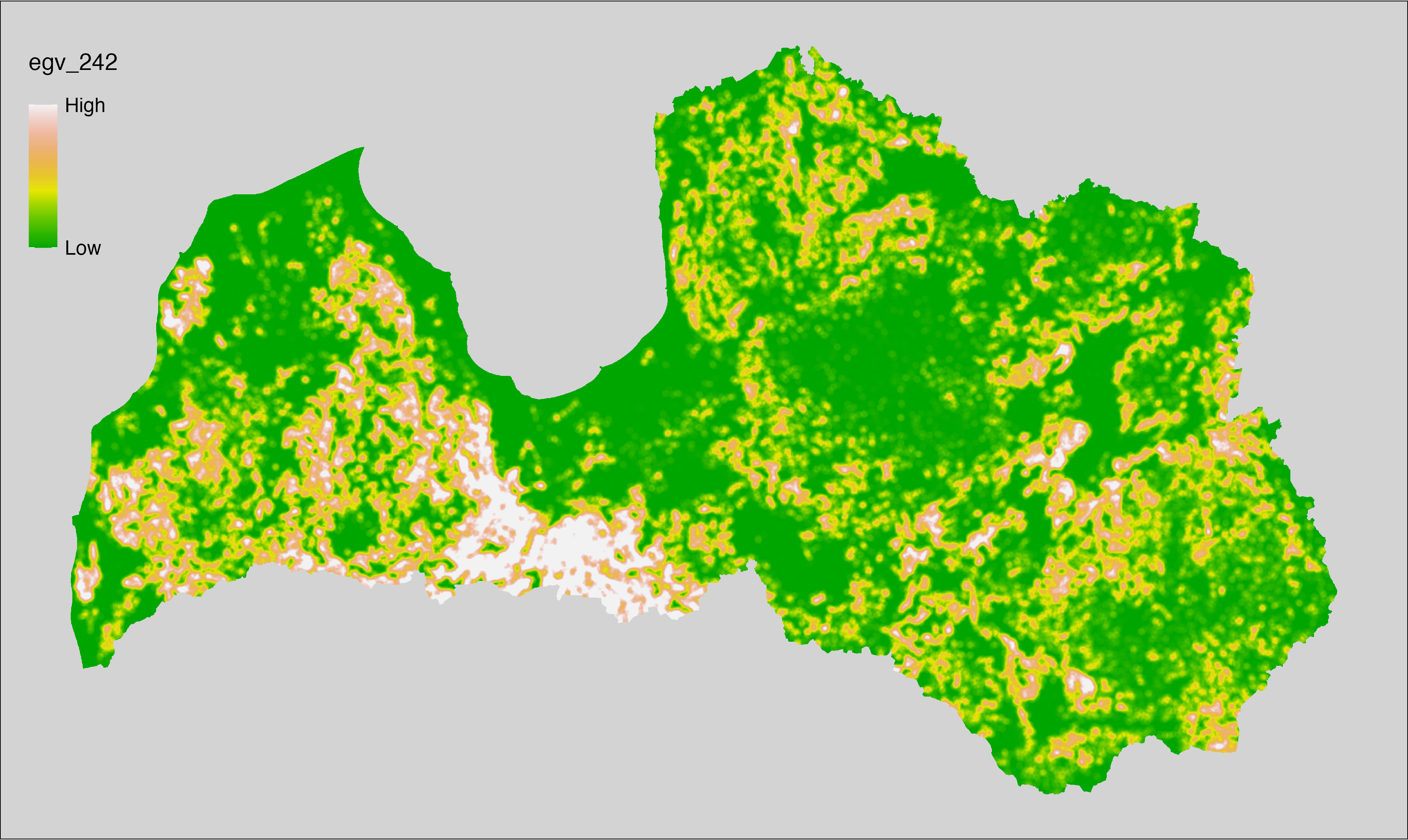
6.243 FarmlandPloughed_CropsFallow_r3000
filename: FarmlandPloughed_CropsFallow_r3000.tif
layername: egv_243
English name: Fractional cover of Crop-, Fallow- Land within the 3 km landscape
Latvian name: Aramzemju, papuvju platības īpatsvars 3 km ainavā
Procedure: The cover fraction within a radius of 3000 m around the analysis grid cell
is calculated as the area-weighted sum of the analysis cells inside
the buffer, using the workflow egvtools::radius_function(). During the calculation of the landscape
metric, inverse distance weighted (power = 2) gap filling on the output is
applied to ensure no missing values at the edges. Then the layer is
rewritten to set its name. Finally, the layer is standardised by
subtracting the arithmetic mean and dividing by the root mean squared error.
Code
# libs ----
if(!require(terra)) {install.packages("terra"); require(terra)}
if(!require(egvtools)) {remotes::install_github("aavotins/egvtools"); require(egvtools)}
# Templates -----
template100=rast("./Templates/TemplateRasters/LV100m_10km.tif")
# radii ----
radius_function(
kvadrati_path = "./Templates/TemplateGrids/tiles/",
radii_path = "./Templates/TemplateGridPoints/tiles/",
tikls100_path = "./Templates/TemplateGrids/tikls100_sauzeme.parquet",
template_path = "./Templates/TemplateRasters/LV100m_10km.tif",
input_layers = c("./RasterGrids_100m/2024/RAW/FarmlandPloughed_CropsFallow_cell.tif"),
layer_prefixes = c("FarmlandPloughed_CropsFallow"),
output_dir = "./RasterGrids_100m/2024/RAW/",
n_workers = 6,
radii = c("r3000"),
radius_mode = "sparse",
extract_fun = "mean",
fill_missing = TRUE,
IDW_weight = 2,
future_max_size = 40 * 1024^3)
# FarmlandPloughed_CropsFallow_r3000.tif egv_243
slanis=rast("./RasterGrids_100m/2024/RAW/FarmlandPloughed_CropsFallow_r3000.tif")
names(slanis)="egv_243"
slanis2=project(slanis,template100)
writeRaster(slanis2,
"./RasterGrids_100m/2024/RAW/FarmlandPloughed_CropsFallow_r3000.tif",
overwrite=TRUE)
# standardisation ----
if(!require(terra)) {install.packages("terra"); require(terra)}
if(!require(tidyverse)) {install.packages("tidyverse"); require(tidyverse)}
nosaukums="FarmlandPloughed_CropsFallow_r3000.tif"
ielasisanas_cels=paste0("./RasterGrids_100m/2024/RAW/",nosaukums)
saglabasanas_cels=paste0("./RasterGrids_100m/2024/Scaled/",nosaukums)
slanis=rast(ielasisanas_cels)
videjais=global(slanis,fun="mean",na.rm=TRUE)
centrets=slanis-videjais[,1]
standartnovirze=terra::global(centrets,fun="rms",na.rm=TRUE)
merogots=centrets/standartnovirze[,1]
writeRaster(merogots,
filename=saglabasanas_cels,
overwrite=TRUE)
6.244 FarmlandPloughed_CropsFallow_r10000
filename: FarmlandPloughed_CropsFallow_r10000.tif
layername: egv_244
English name: Fractional cover of Crop-, Fallow- Land within the 10 km landscape
Latvian name: Aramzemju, papuvju platības īpatsvars 10 km ainavā
Procedure: The cover fraction within a radius of 10000 m around the analysis grid cell
is calculated as the area-weighted sum of the analysis cells inside
the buffer, using the workflow egvtools::radius_function(). During the calculation of the landscape
metric, inverse distance weighted (power = 2) gap filling on the output is
applied to ensure no missing values at the edges. Then the layer is
rewritten to set its name. Finally, the layer is standardised by
subtracting the arithmetic mean and dividing by the root mean squared error.
Code
# libs ----
if(!require(terra)) {install.packages("terra"); require(terra)}
if(!require(egvtools)) {remotes::install_github("aavotins/egvtools"); require(egvtools)}
# Templates -----
template100=rast("./Templates/TemplateRasters/LV100m_10km.tif")
# radii ----
radius_function(
kvadrati_path = "./Templates/TemplateGrids/tiles/",
radii_path = "./Templates/TemplateGridPoints/tiles/",
tikls100_path = "./Templates/TemplateGrids/tikls100_sauzeme.parquet",
template_path = "./Templates/TemplateRasters/LV100m_10km.tif",
input_layers = c("./RasterGrids_100m/2024/RAW/FarmlandPloughed_CropsFallow_cell.tif"),
layer_prefixes = c("FarmlandPloughed_CropsFallow"),
output_dir = "./RasterGrids_100m/2024/RAW/",
n_workers = 6,
radii = c("r10000"),
radius_mode = "sparse",
extract_fun = "mean",
fill_missing = TRUE,
IDW_weight = 2,
future_max_size = 40 * 1024^3)
# FarmlandPloughed_CropsFallow_r10000.tif egv_244
slanis=rast("./RasterGrids_100m/2024/RAW/FarmlandPloughed_CropsFallow_r10000.tif")
names(slanis)="egv_244"
slanis2=project(slanis,template100)
writeRaster(slanis2,
"./RasterGrids_100m/2024/RAW/FarmlandPloughed_CropsFallow_r10000.tif",
overwrite=TRUE)
# standardisation ----
if(!require(terra)) {install.packages("terra"); require(terra)}
if(!require(tidyverse)) {install.packages("tidyverse"); require(tidyverse)}
nosaukums="FarmlandPloughed_CropsFallow_r10000.tif"
ielasisanas_cels=paste0("./RasterGrids_100m/2024/RAW/",nosaukums)
saglabasanas_cels=paste0("./RasterGrids_100m/2024/Scaled/",nosaukums)
slanis=rast(ielasisanas_cels)
videjais=global(slanis,fun="mean",na.rm=TRUE)
centrets=slanis-videjais[,1]
standartnovirze=terra::global(centrets,fun="rms",na.rm=TRUE)
merogots=centrets/standartnovirze[,1]
writeRaster(merogots,
filename=saglabasanas_cels,
overwrite=TRUE)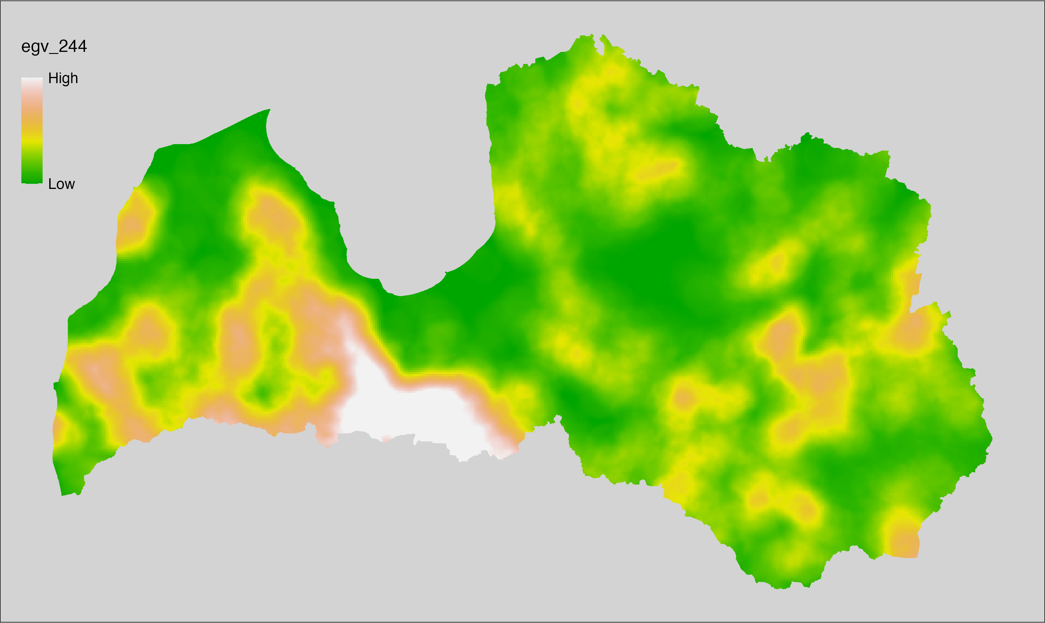
6.245 FarmlandPloughed_CropsFallowTempGrass_cell
filename: FarmlandPloughed_CropsFallowTempGrass_cell.tif
layername: egv_245
English name: Fractional cover of Crop-, Fallow-, Temporary Grass- Lands within the analysis cell (1 ha)
Latvian name: Aramzemju, papuvju, zālāju-aramzemē platības īpatsvars analīzes šūnā (1 ha)
Procedure: First, agricultural parcels declared as crops, fallow land or
grasslands in arable land are selected from the Rural Support Service’s
information on declared fields. Geometries are then rasterised to
input resolution, ensuring value 1 at the polygon locations and value 0
elsewhere. Rasterisation is
performed using the workflow egvtools::polygon2input(). Once rasterised, the
layer is aggregated to EGV resolution using the workflow egvtools::input2egv(),
which calculates the arithmetic mean and thus
results in a cover fraction. During
aggregation, inverse distance weighted (power = 2) gap filling on the output is
applied to ensure no missing values at the edges. Finally, the layer is
standardised by subtracting the arithmetic mean and dividing by the root mean squared
error.
Code
# libs ----
if(!require(egvtools)) {remotes::install_github("aavotins/egvtools"); require(egvtools)}
if(!require(terra)) {install.packages("terra"); require(terra)}
if(!require(sf)) {install.packages("sf"); require(sf)}
if(!require(tidyverse)) {install.packages("tidyverse"); require(tidyverse)}
if(!require(sfarrow)) {install.packages("sfarrow"); require(sfarrow)}
if(!require(readxl)) {install.packages("readxl"); require(readxl)}
if(!require(raster)) {install.packages("raster"); require(raster)}
if(!require(fasterize)) {install.packages("fasterize"); require(fasterize)}
# templates ----
template100=rast("./Templates/TemplateRasters/LV100m_10km.tif")
template10=rast("./Templates/TemplateRasters/LV10m_10km.tif")
rastrs10=raster(template10)
nulls10=rast("./Templates/TemplateRasters/nulls_LV10m_10km.tif")
nulls100=rast("./Templates/TemplateRasters/nulls_LV100m_10km.tif")
# codes ----
kodi=read_excel("./Geodata/2024/LAD/KulturuKodi_2024.xlsx")
kodi$kods=as.character(kodi$kods)
# LAD ----
lad=sfarrow::st_read_parquet("./Geodata/2024/LAD/Lauki_2024.parquet")
lad$yes=1
lad=lad %>%
left_join(kodi,by=c("PRODUCT_CODE"="kods"))
# simple landscape ----
simple_landscape=rast("RasterGrids_10m/2024/Ainava_vienk_mask.tif")
# FarmlandPloughed_CropsFallowTempGrass_cell.tif egv_245 ----
dati=lad %>%
filter(SDM_grupa_sakums %in% c("aramzemes (citur neiekļautās)",
"aramzemes (labība-vasarāji)",
"aramzemes (labība-ziemāji)",
"aramzemes (vagu un rušināmkultūru)",
"aramzemes (vasaras rapsis un rispsis, kukurūzas, zirņi un pupas, soja, kaņepes)",
"aramzemes (ziemas rapsis un ripsis)",
"papuves",
"zālāji (kultivētie)"))
table(dati$SDM_grupa_sakums,useNA="always")
p2i_rez=egvtools::polygon2input(vector_data = dati,
template_path = "./Templates/TemplateRasters/LV10m_10km.tif",
out_path = "./RasterGrids_10m/2024/",
file_name = "FarmlandPloughed_CropsFallowTempGrass_input.tif",
value_field = "yes",
prepare=FALSE,
background_raster = "./Templates/TemplateRasters/nulls_LV10m_10km.tif",
plot_result = TRUE)
p2i_rez
i2e_rez=egvtools::input2egv(input=paste0("./RasterGrids_10m/2024/",
"FarmlandPloughed_CropsFallowTempGrass_input.tif"),
egv_template= "./Templates/TemplateRasters/LV100m_10km.tif",
summary_function = "average",
missing_job = "FillOutput",
outlocation = "./RasterGrids_100m/2024/RAW/",
outfilename = "FarmlandPloughed_CropsFallowTempGrass_cell.tif",
layername = "egv_245",
idw_weight = 2,
plot_gaps = FALSE,plot_final = TRUE)
i2e_rez
rm(p2i_rez)
rm(i2e_rez)
rm(dati)
unlink("./RasterGrids_10m/2024/FarmlandPloughed_CropsFallowTempGrass_input.tif")
# standardisation ----
if(!require(terra)) {install.packages("terra"); require(terra)}
if(!require(tidyverse)) {install.packages("tidyverse"); require(tidyverse)}
nosaukums="FarmlandPloughed_CropsFallowTempGrass_cell.tif"
ielasisanas_cels=paste0("./RasterGrids_100m/2024/RAW/",nosaukums)
saglabasanas_cels=paste0("./RasterGrids_100m/2024/Scaled/",nosaukums)
slanis=rast(ielasisanas_cels)
videjais=global(slanis,fun="mean",na.rm=TRUE)
centrets=slanis-videjais[,1]
standartnovirze=terra::global(centrets,fun="rms",na.rm=TRUE)
merogots=centrets/standartnovirze[,1]
writeRaster(merogots,
filename=saglabasanas_cels,
overwrite=TRUE)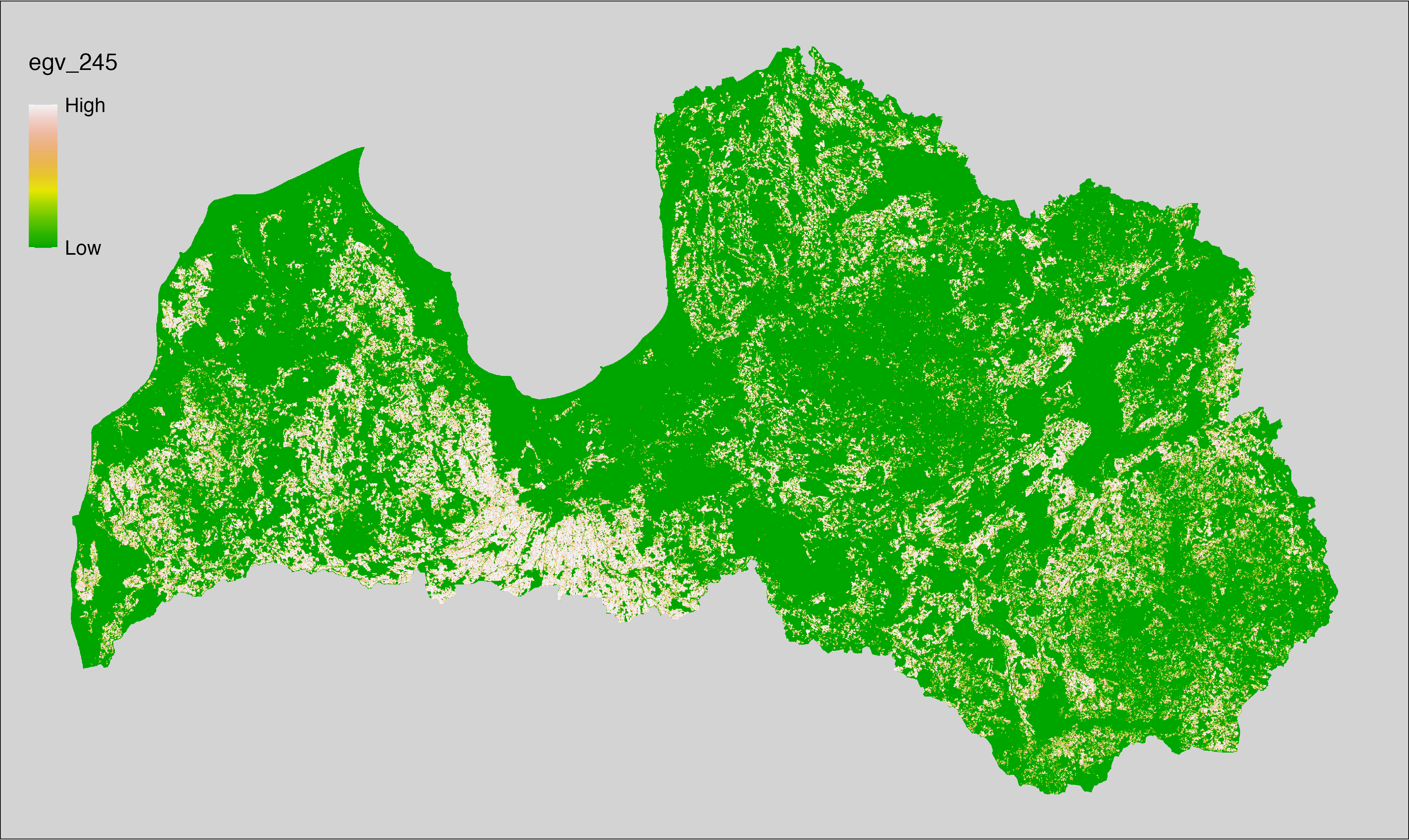
6.246 FarmlandPloughed_CropsFallowTempGrass_r500
filename: FarmlandPloughed_CropsFallowTempGrass_r500.tif
layername: egv_246
English name: Fractional cover of Crop-, Fallow-, Temporary Grass- Lands within the 0.5 km landscape
Latvian name: Aramzemju, papuvju, zālāju-aramzemē platības īpatsvars 0,5 km ainavā
Procedure: The cover fraction within a radius of 500 m around the analysis grid cell is
calculated as the area-weighted sum of the analysis cells inside the
buffer, using the workflow egvtools::radius_function(). During the calculation of the landscape metric,
inverse distance weighted (power = 2) gap filling on the output is applied
to ensure no missing values at the edges. Then the layer is rewritten to set
its name. Finally, the layer is standardised by subtracting the arithmetic
mean and dividing by the root mean squared error.
Code
# libs ----
if(!require(terra)) {install.packages("terra"); require(terra)}
if(!require(egvtools)) {remotes::install_github("aavotins/egvtools"); require(egvtools)}
# Templates -----
template100=rast("./Templates/TemplateRasters/LV100m_10km.tif")
# radii ----
radius_function(
kvadrati_path = "./Templates/TemplateGrids/tiles/",
radii_path = "./Templates/TemplateGridPoints/tiles/",
tikls100_path = "./Templates/TemplateGrids/tikls100_sauzeme.parquet",
template_path = "./Templates/TemplateRasters/LV100m_10km.tif",
input_layers = c("./RasterGrids_100m/2024/RAW/FarmlandPloughed_CropsFallowTempGrass_cell.tif"),
layer_prefixes = c("FarmlandPloughed_CropsFallowTempGrass"),
output_dir = "./RasterGrids_100m/2024/RAW/",
n_workers = 6,
radii = c("r500"),
radius_mode = "sparse",
extract_fun = "mean",
fill_missing = TRUE,
IDW_weight = 2,
future_max_size = 40 * 1024^3)
# FarmlandPloughed_CropsFallowTempGrass_r500.tif egv_246
slanis=rast("./RasterGrids_100m/2024/RAW/FarmlandPloughed_CropsFallowTempGrass_r500.tif")
names(slanis)="egv_246"
slanis2=project(slanis,template100)
writeRaster(slanis2,
"./RasterGrids_100m/2024/RAW/FarmlandPloughed_CropsFallowTempGrass_r500.tif",
overwrite=TRUE)
# standardisation ----
if(!require(terra)) {install.packages("terra"); require(terra)}
if(!require(tidyverse)) {install.packages("tidyverse"); require(tidyverse)}
nosaukums="FarmlandPloughed_CropsFallowTempGrass_r500.tif"
ielasisanas_cels=paste0("./RasterGrids_100m/2024/RAW/",nosaukums)
saglabasanas_cels=paste0("./RasterGrids_100m/2024/Scaled/",nosaukums)
slanis=rast(ielasisanas_cels)
videjais=global(slanis,fun="mean",na.rm=TRUE)
centrets=slanis-videjais[,1]
standartnovirze=terra::global(centrets,fun="rms",na.rm=TRUE)
merogots=centrets/standartnovirze[,1]
writeRaster(merogots,
filename=saglabasanas_cels,
overwrite=TRUE)
6.247 FarmlandPloughed_CropsFallowTempGrass_r1250
filename: FarmlandPloughed_CropsFallowTempGrass_r1250.tif
layername: egv_247
English name: Fractional cover of Crop-, Fallow-, Temporary Grass- Lands within the 1.25 km landscape
Latvian name: Aramzemju, papuvju, zālāju-aramzemē platības īpatsvars 1,25 km ainavā
Procedure: The cover fraction within a radius of 1250 m around the analysis grid cell
is calculated as the area-weighted sum of the analysis cells inside
the buffer, using the workflow egvtools::radius_function(). During the calculation of the landscape
metric, inverse distance weighted (power = 2) gap filling on the output is
applied to ensure no missing values at the edges. Then the layer is
rewritten to set its name. Finally, the layer is standardised by
subtracting the arithmetic mean and dividing by the root mean squared error.
Code
# libs ----
if(!require(terra)) {install.packages("terra"); require(terra)}
if(!require(egvtools)) {remotes::install_github("aavotins/egvtools"); require(egvtools)}
# Templates -----
template100=rast("./Templates/TemplateRasters/LV100m_10km.tif")
# radii ----
radius_function(
kvadrati_path = "./Templates/TemplateGrids/tiles/",
radii_path = "./Templates/TemplateGridPoints/tiles/",
tikls100_path = "./Templates/TemplateGrids/tikls100_sauzeme.parquet",
template_path = "./Templates/TemplateRasters/LV100m_10km.tif",
input_layers = c("./RasterGrids_100m/2024/RAW/FarmlandPloughed_CropsFallowTempGrass_cell.tif"),
layer_prefixes = c("FarmlandPloughed_CropsFallowTempGrass"),
output_dir = "./RasterGrids_100m/2024/RAW/",
n_workers = 6,
radii = c("r1250"),
radius_mode = "sparse",
extract_fun = "mean",
fill_missing = TRUE,
IDW_weight = 2,
future_max_size = 40 * 1024^3)
# FarmlandPloughed_CropsFallowTempGrass_r1250.tif egv_247
slanis=rast("./RasterGrids_100m/2024/RAW/FarmlandPloughed_CropsFallowTempGrass_r1250.tif")
names(slanis)="egv_247"
slanis2=project(slanis,template100)
writeRaster(slanis2,
"./RasterGrids_100m/2024/RAW/FarmlandPloughed_CropsFallowTempGrass_r1250.tif",
overwrite=TRUE)
# standardisation ----
if(!require(terra)) {install.packages("terra"); require(terra)}
if(!require(tidyverse)) {install.packages("tidyverse"); require(tidyverse)}
nosaukums="FarmlandPloughed_CropsFallowTempGrass_r1250.tif"
ielasisanas_cels=paste0("./RasterGrids_100m/2024/RAW/",nosaukums)
saglabasanas_cels=paste0("./RasterGrids_100m/2024/Scaled/",nosaukums)
slanis=rast(ielasisanas_cels)
videjais=global(slanis,fun="mean",na.rm=TRUE)
centrets=slanis-videjais[,1]
standartnovirze=terra::global(centrets,fun="rms",na.rm=TRUE)
merogots=centrets/standartnovirze[,1]
writeRaster(merogots,
filename=saglabasanas_cels,
overwrite=TRUE)
6.248 FarmlandPloughed_CropsFallowTempGrass_r3000
filename: FarmlandPloughed_CropsFallowTempGrass_r3000.tif
layername: egv_248
English name: Fractional cover of Crop-, Fallow-, Temporary Grass- Lands within the 3 km landscape
Latvian name: Aramzemju, papuvju, zālāju-aramzemē platības īpatsvars 3 km ainavā
Procedure: The cover fraction within a radius of 3000 m around the analysis grid cell
is calculated as the area-weighted sum of the analysis cells inside
the buffer, using the workflow egvtools::radius_function(). During the calculation of the landscape
metric, inverse distance weighted (power = 2) gap filling on the output is
applied to ensure no missing values at the edges. Then the layer is
rewritten to set its name. Finally, the layer is standardised by
subtracting the arithmetic mean and dividing by the root mean squared error.
Code
# libs ----
if(!require(terra)) {install.packages("terra"); require(terra)}
if(!require(egvtools)) {remotes::install_github("aavotins/egvtools"); require(egvtools)}
# Templates -----
template100=rast("./Templates/TemplateRasters/LV100m_10km.tif")
# radii ----
radius_function(
kvadrati_path = "./Templates/TemplateGrids/tiles/",
radii_path = "./Templates/TemplateGridPoints/tiles/",
tikls100_path = "./Templates/TemplateGrids/tikls100_sauzeme.parquet",
template_path = "./Templates/TemplateRasters/LV100m_10km.tif",
input_layers = c("./RasterGrids_100m/2024/RAW/FarmlandPloughed_CropsFallowTempGrass_cell.tif"),
layer_prefixes = c("FarmlandPloughed_CropsFallowTempGrass"),
output_dir = "./RasterGrids_100m/2024/RAW/",
n_workers = 6,
radii = c("r3000"),
radius_mode = "sparse",
extract_fun = "mean",
fill_missing = TRUE,
IDW_weight = 2,
future_max_size = 40 * 1024^3)
# FarmlandPloughed_CropsFallowTempGrass_r3000.tif egv_248
slanis=rast("./RasterGrids_100m/2024/RAW/FarmlandPloughed_CropsFallowTempGrass_r3000.tif")
names(slanis)="egv_248"
slanis2=project(slanis,template100)
writeRaster(slanis2,
"./RasterGrids_100m/2024/RAW/FarmlandPloughed_CropsFallowTempGrass_r3000.tif",
overwrite=TRUE)
# standardisation ----
if(!require(terra)) {install.packages("terra"); require(terra)}
if(!require(tidyverse)) {install.packages("tidyverse"); require(tidyverse)}
nosaukums="FarmlandPloughed_CropsFallowTempGrass_r3000.tif"
ielasisanas_cels=paste0("./RasterGrids_100m/2024/RAW/",nosaukums)
saglabasanas_cels=paste0("./RasterGrids_100m/2024/Scaled/",nosaukums)
slanis=rast(ielasisanas_cels)
videjais=global(slanis,fun="mean",na.rm=TRUE)
centrets=slanis-videjais[,1]
standartnovirze=terra::global(centrets,fun="rms",na.rm=TRUE)
merogots=centrets/standartnovirze[,1]
writeRaster(merogots,
filename=saglabasanas_cels,
overwrite=TRUE)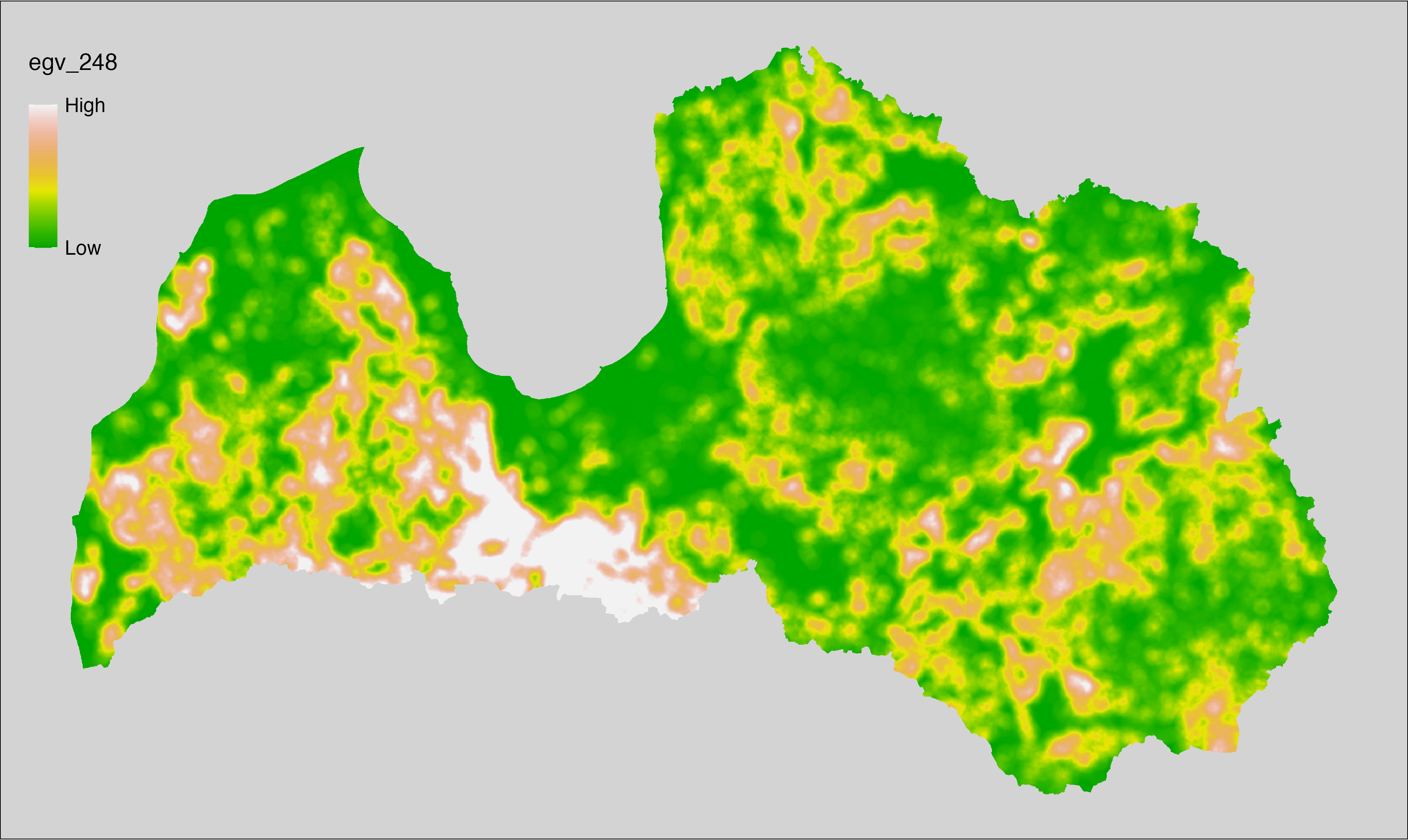
6.249 FarmlandPloughed_CropsFallowTempGrass_r10000
filename: FarmlandPloughed_CropsFallowTempGrass_r10000.tif
layername: egv_249
English name: Fractional cover of Crop-, Fallow-, Temporary Grass- Lands within the 10 km landscape
Latvian name: Aramzemju, papuvju, zālāju-aramzemē platības īpatsvars 10 km ainavā
Procedure: The cover fraction within a radius of 10000 m around the analysis grid cell
is calculated as the area-weighted sum of the analysis cells inside
the buffer, using the workflow egvtools::radius_function(). During the calculation of the landscape
metric, inverse distance weighted (power = 2) gap filling on the output is
applied to ensure no missing values at the edges. Then the layer is
rewritten to set its name. Finally, the layer is standardised by
subtracting the arithmetic mean and dividing by the root mean squared error.
Code
# libs ----
if(!require(terra)) {install.packages("terra"); require(terra)}
if(!require(egvtools)) {remotes::install_github("aavotins/egvtools"); require(egvtools)}
# Templates -----
template100=rast("./Templates/TemplateRasters/LV100m_10km.tif")
# radii ----
radius_function(
kvadrati_path = "./Templates/TemplateGrids/tiles/",
radii_path = "./Templates/TemplateGridPoints/tiles/",
tikls100_path = "./Templates/TemplateGrids/tikls100_sauzeme.parquet",
template_path = "./Templates/TemplateRasters/LV100m_10km.tif",
input_layers = c("./RasterGrids_100m/2024/RAW/FarmlandPloughed_CropsFallowTempGrass_cell.tif"),
layer_prefixes = c("FarmlandPloughed_CropsFallowTempGrass"),
output_dir = "./RasterGrids_100m/2024/RAW/",
n_workers = 6,
radii = c("r10000"),
radius_mode = "sparse",
extract_fun = "mean",
fill_missing = TRUE,
IDW_weight = 2,
future_max_size = 40 * 1024^3)
# FarmlandPloughed_CropsFallowTempGrass_r10000.tif egv_249
slanis=rast("./RasterGrids_100m/2024/RAW/FarmlandPloughed_CropsFallowTempGrass_r10000.tif")
names(slanis)="egv_249"
slanis2=project(slanis,template100)
writeRaster(slanis2,
"./RasterGrids_100m/2024/RAW/FarmlandPloughed_CropsFallowTempGrass_r10000.tif",
overwrite=TRUE)
# standardisation ----
if(!require(terra)) {install.packages("terra"); require(terra)}
if(!require(tidyverse)) {install.packages("tidyverse"); require(tidyverse)}
nosaukums="FarmlandPloughed_CropsFallowTempGrass_r10000.tif"
ielasisanas_cels=paste0("./RasterGrids_100m/2024/RAW/",nosaukums)
saglabasanas_cels=paste0("./RasterGrids_100m/2024/Scaled/",nosaukums)
slanis=rast(ielasisanas_cels)
videjais=global(slanis,fun="mean",na.rm=TRUE)
centrets=slanis-videjais[,1]
standartnovirze=terra::global(centrets,fun="rms",na.rm=TRUE)
merogots=centrets/standartnovirze[,1]
writeRaster(merogots,
filename=saglabasanas_cels,
overwrite=TRUE)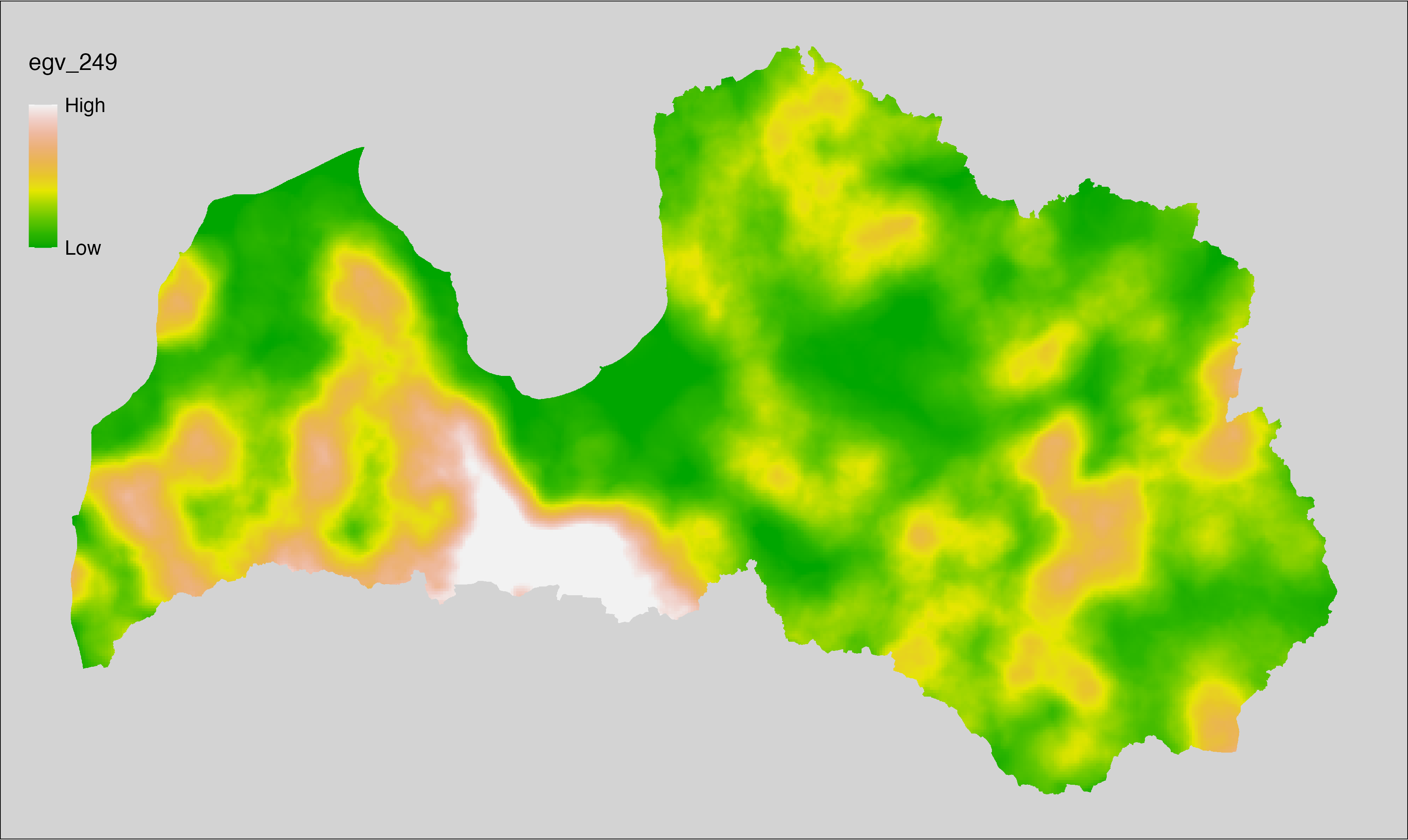
6.250 FarmlandPloughed_Fallow_cell
filename: FarmlandPloughed_Fallow_cell.tif
layername: egv_250
English name: Fractional cover of Fallow Land within the analysis cell (1 ha)
Latvian name: Papuvju platības īpatsvars analīzes šūnā (1 ha)
Procedure: First, agricultural parcels declared as fallow land are selected
from the Rural Support Service’s information on declared fields.
Geometries are then rasterised to input resolution, ensuring value 1 at the
polygon locations and value 0 elsewhere. Rasterisation is
performed using the workflow egvtools::polygon2input(). Once rasterised, the
layer is aggregated to EGV resolution using the workflow egvtools::input2egv(),
which calculates the arithmetic mean and thus
results in a cover fraction. During aggregation, inverse distance weighted
(power = 2) gap filling on the output is applied to ensure no missing
values at the edges. Finally, the layer is standardised by subtracting
the arithmetic mean and dividing by the root mean squared error.
Code
# libs ----
if(!require(egvtools)) {remotes::install_github("aavotins/egvtools"); require(egvtools)}
if(!require(terra)) {install.packages("terra"); require(terra)}
if(!require(sf)) {install.packages("sf"); require(sf)}
if(!require(tidyverse)) {install.packages("tidyverse"); require(tidyverse)}
if(!require(sfarrow)) {install.packages("sfarrow"); require(sfarrow)}
if(!require(readxl)) {install.packages("readxl"); require(readxl)}
if(!require(raster)) {install.packages("raster"); require(raster)}
if(!require(fasterize)) {install.packages("fasterize"); require(fasterize)}
# templates ----
template100=rast("./Templates/TemplateRasters/LV100m_10km.tif")
template10=rast("./Templates/TemplateRasters/LV10m_10km.tif")
rastrs10=raster(template10)
nulls10=rast("./Templates/TemplateRasters/nulls_LV10m_10km.tif")
nulls100=rast("./Templates/TemplateRasters/nulls_LV100m_10km.tif")
# codes ----
kodi=read_excel("./Geodata/2024/LAD/KulturuKodi_2024.xlsx")
kodi$kods=as.character(kodi$kods)
# LAD ----
lad=sfarrow::st_read_parquet("./Geodata/2024/LAD/Lauki_2024.parquet")
lad$yes=1
lad=lad %>%
left_join(kodi,by=c("PRODUCT_CODE"="kods"))
# simple landscape ----
simple_landscape=rast("RasterGrids_10m/2024/Ainava_vienk_mask.tif")
# FarmlandPloughed_Fallow_cell.tif egv_250 ----
dati=lad %>%
filter(SDM_grupa_sakums == "papuves")
table(dati$SDM_grupa_sakums,useNA="always")
p2i_rez=egvtools::polygon2input(vector_data = dati,
template_path = "./Templates/TemplateRasters/LV10m_10km.tif",
out_path = "./RasterGrids_10m/2024/",
file_name = "FarmlandPloughed_Fallow_input.tif",
value_field = "yes",
prepare=FALSE,
background_raster = "./Templates/TemplateRasters/nulls_LV10m_10km.tif",
plot_result = TRUE)
p2i_rez
i2e_rez=egvtools::input2egv(input=paste0("./RasterGrids_10m/2024/",
"FarmlandPloughed_Fallow_input.tif"),
egv_template= "./Templates/TemplateRasters/LV100m_10km.tif",
summary_function = "average",
missing_job = "FillOutput",
outlocation = "./RasterGrids_100m/2024/RAW/",
outfilename = "FarmlandPloughed_Fallow_cell.tif",
layername = "egv_250",
idw_weight = 2,
plot_gaps = FALSE,plot_final = TRUE)
i2e_rez
rm(p2i_rez)
rm(i2e_rez)
rm(dati)
unlink("./RasterGrids_10m/2024/FarmlandPloughed_Fallow_input.tif")
# standardisation ----
if(!require(terra)) {install.packages("terra"); require(terra)}
if(!require(tidyverse)) {install.packages("tidyverse"); require(tidyverse)}
nosaukums="FarmlandPloughed_Fallow_cell.tif"
ielasisanas_cels=paste0("./RasterGrids_100m/2024/RAW/",nosaukums)
saglabasanas_cels=paste0("./RasterGrids_100m/2024/Scaled/",nosaukums)
slanis=rast(ielasisanas_cels)
videjais=global(slanis,fun="mean",na.rm=TRUE)
centrets=slanis-videjais[,1]
standartnovirze=terra::global(centrets,fun="rms",na.rm=TRUE)
merogots=centrets/standartnovirze[,1]
writeRaster(merogots,
filename=saglabasanas_cels,
overwrite=TRUE)
6.251 FarmlandPloughed_Fallow_r500
filename: FarmlandPloughed_Fallow_r500.tif
layername: egv_251
English name: Fractional cover of Fallow Land within the 0.5 km landscape
Latvian name: Papuvju platības īpatsvars 0,5 km ainavā
Procedure: The cover fraction within a radius of 500 m around the analysis grid cell is
calculated as the area-weighted sum of the analysis cells inside the
buffer, using the workflow egvtools::radius_function(). During the calculation of the landscape metric,
inverse distance weighted (power = 2) gap filling on the output is applied
to ensure no missing values at the edges. Then the layer is rewritten to set
its name. Finally, the layer is standardised by subtracting the arithmetic
mean and dividing by the root mean squared error.
Code
# libs ----
if(!require(terra)) {install.packages("terra"); require(terra)}
if(!require(egvtools)) {remotes::install_github("aavotins/egvtools"); require(egvtools)}
# Templates -----
template100=rast("./Templates/TemplateRasters/LV100m_10km.tif")
# radii ----
radius_function(
kvadrati_path = "./Templates/TemplateGrids/tiles/",
radii_path = "./Templates/TemplateGridPoints/tiles/",
tikls100_path = "./Templates/TemplateGrids/tikls100_sauzeme.parquet",
template_path = "./Templates/TemplateRasters/LV100m_10km.tif",
input_layers = c("./RasterGrids_100m/2024/RAW/FarmlandPloughed_Fallow_cell.tif"),
layer_prefixes = c("FarmlandPloughed_Fallow"),
output_dir = "./RasterGrids_100m/2024/RAW/",
n_workers = 6,
radii = c("r500"),
radius_mode = "sparse",
extract_fun = "mean",
fill_missing = TRUE,
IDW_weight = 2,
future_max_size = 40 * 1024^3)
# FarmlandPloughed_Fallow_r500.tif egv_251
slanis=rast("./RasterGrids_100m/2024/RAW/FarmlandPloughed_Fallow_r500.tif")
names(slanis)="egv_251"
slanis2=project(slanis,template100)
writeRaster(slanis2,
"./RasterGrids_100m/2024/RAW/FarmlandPloughed_Fallow_r500.tif",
overwrite=TRUE)
# standardisation ----
if(!require(terra)) {install.packages("terra"); require(terra)}
if(!require(tidyverse)) {install.packages("tidyverse"); require(tidyverse)}
nosaukums="FarmlandPloughed_Fallow_r500.tif"
ielasisanas_cels=paste0("./RasterGrids_100m/2024/RAW/",nosaukums)
saglabasanas_cels=paste0("./RasterGrids_100m/2024/Scaled/",nosaukums)
slanis=rast(ielasisanas_cels)
videjais=global(slanis,fun="mean",na.rm=TRUE)
centrets=slanis-videjais[,1]
standartnovirze=terra::global(centrets,fun="rms",na.rm=TRUE)
merogots=centrets/standartnovirze[,1]
writeRaster(merogots,
filename=saglabasanas_cels,
overwrite=TRUE)
6.252 FarmlandPloughed_Fallow_r1250
filename: FarmlandPloughed_Fallow_r1250.tif
layername: egv_252
English name: Fractional cover of Fallow Land within the 1.25 km landscape
Latvian name: Papuvju platības īpatsvars 1,25 km ainavā
Procedure: The cover fraction within a radius of 1250 m around the analysis grid cell
is calculated as the area-weighted sum of the analysis cells inside
the buffer, using the workflow egvtools::radius_function(). During the calculation of the landscape
metric, inverse distance weighted (power = 2) gap filling on the output is
applied to ensure no missing values at the edges. Then the layer is
rewritten to set its name. Finally, the layer is standardised by
subtracting the arithmetic mean and dividing by the root mean squared error.
Code
# libs ----
if(!require(terra)) {install.packages("terra"); require(terra)}
if(!require(egvtools)) {remotes::install_github("aavotins/egvtools"); require(egvtools)}
# Templates -----
template100=rast("./Templates/TemplateRasters/LV100m_10km.tif")
# radii ----
radius_function(
kvadrati_path = "./Templates/TemplateGrids/tiles/",
radii_path = "./Templates/TemplateGridPoints/tiles/",
tikls100_path = "./Templates/TemplateGrids/tikls100_sauzeme.parquet",
template_path = "./Templates/TemplateRasters/LV100m_10km.tif",
input_layers = c("./RasterGrids_100m/2024/RAW/FarmlandPloughed_Fallow_cell.tif"),
layer_prefixes = c("FarmlandPloughed_Fallow"),
output_dir = "./RasterGrids_100m/2024/RAW/",
n_workers = 6,
radii = c("r1250"),
radius_mode = "sparse",
extract_fun = "mean",
fill_missing = TRUE,
IDW_weight = 2,
future_max_size = 40 * 1024^3)
# FarmlandPloughed_Fallow_r1250.tif egv_252
slanis=rast("./RasterGrids_100m/2024/RAW/FarmlandPloughed_Fallow_r1250.tif")
names(slanis)="egv_252"
slanis2=project(slanis,template100)
writeRaster(slanis2,
"./RasterGrids_100m/2024/RAW/FarmlandPloughed_Fallow_r1250.tif",
overwrite=TRUE)
# standardisation ----
if(!require(terra)) {install.packages("terra"); require(terra)}
if(!require(tidyverse)) {install.packages("tidyverse"); require(tidyverse)}
nosaukums="FarmlandPloughed_Fallow_r1250.tif"
ielasisanas_cels=paste0("./RasterGrids_100m/2024/RAW/",nosaukums)
saglabasanas_cels=paste0("./RasterGrids_100m/2024/Scaled/",nosaukums)
slanis=rast(ielasisanas_cels)
videjais=global(slanis,fun="mean",na.rm=TRUE)
centrets=slanis-videjais[,1]
standartnovirze=terra::global(centrets,fun="rms",na.rm=TRUE)
merogots=centrets/standartnovirze[,1]
writeRaster(merogots,
filename=saglabasanas_cels,
overwrite=TRUE)
6.253 FarmlandPloughed_Fallow_r3000
filename: FarmlandPloughed_Fallow_r3000.tif
layername: egv_253
English name: Fractional cover of Fallow Land within the 3 km landscape
Latvian name: Papuvju platības īpatsvars 3 km ainavā
Procedure: The cover fraction within a radius of 3000 m around the analysis grid cell
is calculated as the area-weighted sum of the analysis cells inside
the buffer, using the workflow egvtools::radius_function(). During the calculation of the landscape
metric, inverse distance weighted (power = 2) gap filling on the output is
applied to ensure no missing values at the edges. Then the layer is
rewritten to set its name. Finally, the layer is standardised by
subtracting the arithmetic mean and dividing by the root mean squared error.
Code
# libs ----
if(!require(terra)) {install.packages("terra"); require(terra)}
if(!require(egvtools)) {remotes::install_github("aavotins/egvtools"); require(egvtools)}
# Templates -----
template100=rast("./Templates/TemplateRasters/LV100m_10km.tif")
# radii ----
radius_function(
kvadrati_path = "./Templates/TemplateGrids/tiles/",
radii_path = "./Templates/TemplateGridPoints/tiles/",
tikls100_path = "./Templates/TemplateGrids/tikls100_sauzeme.parquet",
template_path = "./Templates/TemplateRasters/LV100m_10km.tif",
input_layers = c("./RasterGrids_100m/2024/RAW/FarmlandPloughed_Fallow_cell.tif"),
layer_prefixes = c("FarmlandPloughed_Fallow"),
output_dir = "./RasterGrids_100m/2024/RAW/",
n_workers = 6,
radii = c("r3000"),
radius_mode = "sparse",
extract_fun = "mean",
fill_missing = TRUE,
IDW_weight = 2,
future_max_size = 40 * 1024^3)
# FarmlandPloughed_Fallow_r3000.tif egv_253
slanis=rast("./RasterGrids_100m/2024/RAW/FarmlandPloughed_Fallow_r3000.tif")
names(slanis)="egv_253"
slanis2=project(slanis,template100)
writeRaster(slanis2,
"./RasterGrids_100m/2024/RAW/FarmlandPloughed_Fallow_r3000.tif",
overwrite=TRUE)
# standardisation ----
if(!require(terra)) {install.packages("terra"); require(terra)}
if(!require(tidyverse)) {install.packages("tidyverse"); require(tidyverse)}
nosaukums="FarmlandPloughed_Fallow_r3000.tif"
ielasisanas_cels=paste0("./RasterGrids_100m/2024/RAW/",nosaukums)
saglabasanas_cels=paste0("./RasterGrids_100m/2024/Scaled/",nosaukums)
slanis=rast(ielasisanas_cels)
videjais=global(slanis,fun="mean",na.rm=TRUE)
centrets=slanis-videjais[,1]
standartnovirze=terra::global(centrets,fun="rms",na.rm=TRUE)
merogots=centrets/standartnovirze[,1]
writeRaster(merogots,
filename=saglabasanas_cels,
overwrite=TRUE)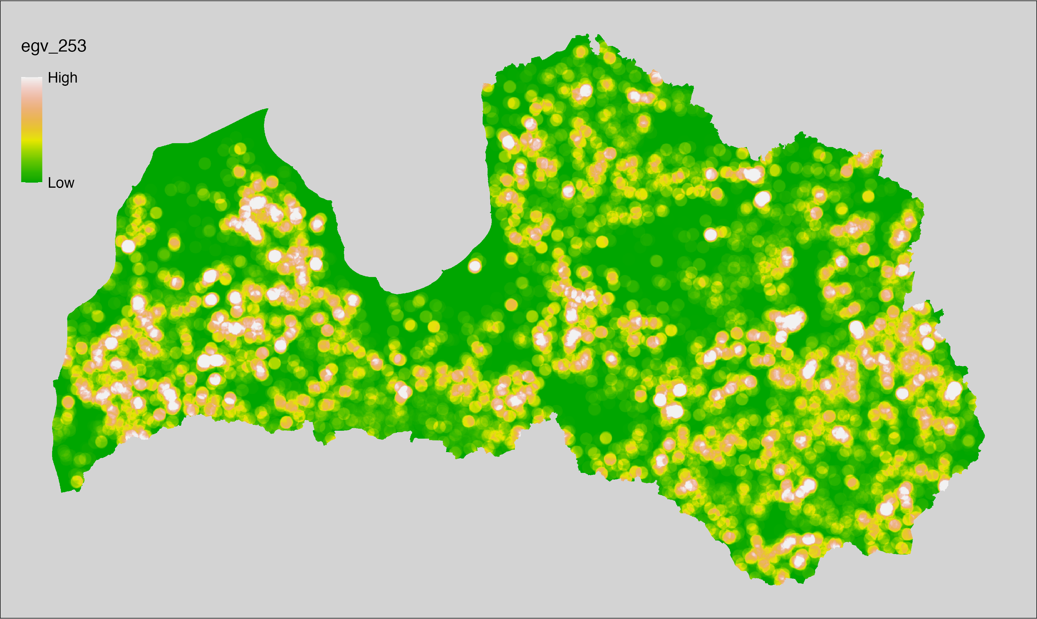
6.254 FarmlandPloughed_Fallow_r10000
filename: FarmlandPloughed_Fallow_r10000.tif
layername: egv_254
English name: Fractional cover of Fallow Land within the 10 km landscape
Latvian name: Papuvju platības īpatsvars 10 km ainavā
Procedure: The cover fraction within a radius of 10000 m around the analysis grid cell
is calculated as the area-weighted sum of the analysis cells inside
the buffer, using the workflow egvtools::radius_function(). During the calculation of the landscape
metric, inverse distance weighted (power = 2) gap filling on the output is
applied to ensure no missing values at the edges. Then the layer is
rewritten to set its name. Finally, the layer is standardised by
subtracting the arithmetic mean and dividing by the root mean squared error.
Code
# libs ----
if(!require(terra)) {install.packages("terra"); require(terra)}
if(!require(egvtools)) {remotes::install_github("aavotins/egvtools"); require(egvtools)}
# Templates -----
template100=rast("./Templates/TemplateRasters/LV100m_10km.tif")
# radii ----
radius_function(
kvadrati_path = "./Templates/TemplateGrids/tiles/",
radii_path = "./Templates/TemplateGridPoints/tiles/",
tikls100_path = "./Templates/TemplateGrids/tikls100_sauzeme.parquet",
template_path = "./Templates/TemplateRasters/LV100m_10km.tif",
input_layers = c("./RasterGrids_100m/2024/RAW/FarmlandPloughed_Fallow_cell.tif"),
layer_prefixes = c("FarmlandPloughed_Fallow"),
output_dir = "./RasterGrids_100m/2024/RAW/",
n_workers = 6,
radii = c("r10000"),
radius_mode = "sparse",
extract_fun = "mean",
fill_missing = TRUE,
IDW_weight = 2,
future_max_size = 40 * 1024^3)
# FarmlandPloughed_Fallow_r10000.tif egv_254
slanis=rast("./RasterGrids_100m/2024/RAW/FarmlandPloughed_Fallow_r10000.tif")
names(slanis)="egv_254"
slanis2=project(slanis,template100)
writeRaster(slanis2,
"./RasterGrids_100m/2024/RAW/FarmlandPloughed_Fallow_r10000.tif",
overwrite=TRUE)
# standardisation ----
if(!require(terra)) {install.packages("terra"); require(terra)}
if(!require(tidyverse)) {install.packages("tidyverse"); require(tidyverse)}
nosaukums="FarmlandPloughed_Fallow_r10000.tif"
ielasisanas_cels=paste0("./RasterGrids_100m/2024/RAW/",nosaukums)
saglabasanas_cels=paste0("./RasterGrids_100m/2024/Scaled/",nosaukums)
slanis=rast(ielasisanas_cels)
videjais=global(slanis,fun="mean",na.rm=TRUE)
centrets=slanis-videjais[,1]
standartnovirze=terra::global(centrets,fun="rms",na.rm=TRUE)
merogots=centrets/standartnovirze[,1]
writeRaster(merogots,
filename=saglabasanas_cels,
overwrite=TRUE)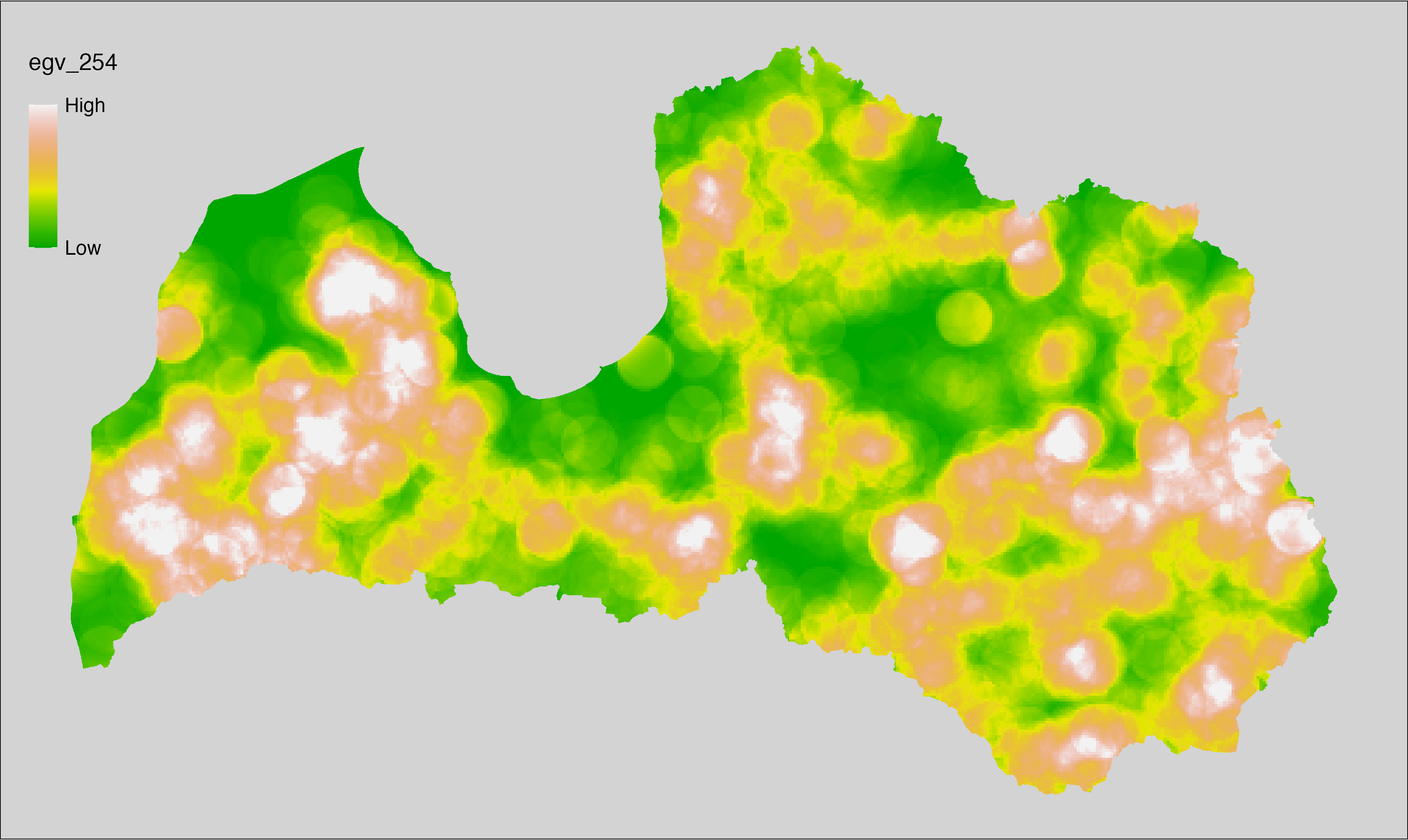
6.255 FarmlandSubsidies_BiologicalSubsidies_cell
filename: FarmlandSubsidies_BiologicalSubsidies_cell.tif
layername: egv_255
English name: Fractional cover of Farmland receiving Subsidies for Biological Agriculture within the analysis cell (1 ha)
Latvian name: Bioloģiskās lauksaimniecības atbalstam pieteikto lauksaimniecības platību īpatsvars analīzes šūnā (1 ha)
Procedure: First, agricultural parcels declared as receiving subsidies for
biological agriculture are selected from the Rural Support Service’s information
on declared fields. Geometries are then rasterised to input
resolution, ensuring value 1 at the polygon locations and value 0 elsewhere.
Rasterisation is
performed using the workflow egvtools::polygon2input(). Once rasterised, the
layer is aggregated to EGV resolution using the workflow egvtools::input2egv(),
which calculates the arithmetic mean and thus
results in a cover fraction. During
aggregation, inverse distance weighted (power = 2) gap filling on the output is
applied to ensure no missing values at the edges. Finally, the layer is
standardised by subtracting the arithmetic mean and dividing by the root mean squared
error.
Code
# libs ----
if(!require(egvtools)) {remotes::install_github("aavotins/egvtools"); require(egvtools)}
if(!require(terra)) {install.packages("terra"); require(terra)}
if(!require(sf)) {install.packages("sf"); require(sf)}
if(!require(tidyverse)) {install.packages("tidyverse"); require(tidyverse)}
if(!require(sfarrow)) {install.packages("sfarrow"); require(sfarrow)}
if(!require(readxl)) {install.packages("readxl"); require(readxl)}
if(!require(raster)) {install.packages("raster"); require(raster)}
if(!require(fasterize)) {install.packages("fasterize"); require(fasterize)}
# templates ----
template100=rast("./Templates/TemplateRasters/LV100m_10km.tif")
template10=rast("./Templates/TemplateRasters/LV10m_10km.tif")
rastrs10=raster(template10)
nulls10=rast("./Templates/TemplateRasters/nulls_LV10m_10km.tif")
nulls100=rast("./Templates/TemplateRasters/nulls_LV100m_10km.tif")
# codes ----
kodi=read_excel("./Geodata/2024/LAD/KulturuKodi_2024.xlsx")
kodi$kods=as.character(kodi$kods)
# LAD ----
lad=sfarrow::st_read_parquet("./Geodata/2024/LAD/Lauki_2024.parquet")
lad$yes=1
lad=lad %>%
left_join(kodi,by=c("PRODUCT_CODE"="kods"))
# simple landscape ----
simple_landscape=rast("RasterGrids_10m/2024/Ainava_vienk_mask.tif")
# FarmlandSubsidies_BiologicalSubsidies_cell.tif egv_255 ----
dati=lad %>%
filter(str_detect(AID_FORMS,"BLA"))
table(dati$AID_FORMS,useNA="always")
p2i_rez=egvtools::polygon2input(vector_data = dati,
template_path = "./Templates/TemplateRasters/LV10m_10km.tif",
out_path = "./RasterGrids_10m/2024/",
file_name = "FarmlandSubsidies_BiologicalSubsidies_input.tif",
value_field = "yes",
prepare=FALSE,
background_raster = "./Templates/TemplateRasters/nulls_LV10m_10km.tif",
plot_result = TRUE)
p2i_rez
i2e_rez=egvtools::input2egv(input=paste0("./RasterGrids_10m/2024/",
"FarmlandSubsidies_BiologicalSubsidies_input.tif"),
egv_template= "./Templates/TemplateRasters/LV100m_10km.tif",
summary_function = "average",
missing_job = "FillOutput",
outlocation = "./RasterGrids_100m/2024/RAW/",
outfilename = "FarmlandSubsidies_BiologicalSubsidies_cell.tif",
layername = "egv_255",
idw_weight = 2,
plot_gaps = FALSE,plot_final = TRUE)
i2e_rez
rm(p2i_rez)
rm(i2e_rez)
rm(dati)
unlink("./RasterGrids_10m/2024/FarmlandSubsidies_BiologicalSubsidies_input.tif")
# standardisation ----
if(!require(terra)) {install.packages("terra"); require(terra)}
if(!require(tidyverse)) {install.packages("tidyverse"); require(tidyverse)}
nosaukums="FarmlandSubsidies_BiologicalSubsidies_cell.tif"
ielasisanas_cels=paste0("./RasterGrids_100m/2024/RAW/",nosaukums)
saglabasanas_cels=paste0("./RasterGrids_100m/2024/Scaled/",nosaukums)
slanis=rast(ielasisanas_cels)
videjais=global(slanis,fun="mean",na.rm=TRUE)
centrets=slanis-videjais[,1]
standartnovirze=terra::global(centrets,fun="rms",na.rm=TRUE)
merogots=centrets/standartnovirze[,1]
writeRaster(merogots,
filename=saglabasanas_cels,
overwrite=TRUE)
6.256 FarmlandSubsidies_BiologicalSubsidies_r500
filename: FarmlandSubsidies_BiologicalSubsidies_r500.tif
layername: egv_256
English name: Fractional cover of Farmland receiving Subsidies for Biological Agriculture within the 0.5 km landscape
Latvian name: Bioloģiskās lauksaimniecības atbalstam pieteikto lauksaimniecības platību īpatsvars 0,5 km ainavā
Procedure: The cover fraction within a radius of 500 m around the analysis grid cell is
calculated as the area-weighted sum of the analysis cells inside the
buffer, using the workflow egvtools::radius_function(). During the calculation of the landscape metric,
inverse distance weighted (power = 2) gap filling on the output is applied
to ensure no missing values at the edges. Then the layer is rewritten to set
its name. Finally, the layer is standardised by subtracting the arithmetic
mean and dividing by the root mean squared error.
Code
# libs ----
if(!require(terra)) {install.packages("terra"); require(terra)}
if(!require(egvtools)) {remotes::install_github("aavotins/egvtools"); require(egvtools)}
# Templates -----
template100=rast("./Templates/TemplateRasters/LV100m_10km.tif")
# radii ----
radius_function(
kvadrati_path = "./Templates/TemplateGrids/tiles/",
radii_path = "./Templates/TemplateGridPoints/tiles/",
tikls100_path = "./Templates/TemplateGrids/tikls100_sauzeme.parquet",
template_path = "./Templates/TemplateRasters/LV100m_10km.tif",
input_layers = c("./RasterGrids_100m/2024/RAW/FarmlandSubsidies_BiologicalSubsidies_cell.tif"),
layer_prefixes = c("FarmlandSubsidies_BiologicalSubsidies"),
output_dir = "./RasterGrids_100m/2024/RAW/",
n_workers = 6,
radii = c("r500"),
radius_mode = "sparse",
extract_fun = "mean",
fill_missing = TRUE,
IDW_weight = 2,
future_max_size = 40 * 1024^3)
# FarmlandSubsidies_BiologicalSubsidies_r500.tif egv_256
slanis=rast("./RasterGrids_100m/2024/RAW/FarmlandSubsidies_BiologicalSubsidies_r500.tif")
names(slanis)="egv_256"
slanis2=project(slanis,template100)
writeRaster(slanis2,
"./RasterGrids_100m/2024/RAW/FarmlandSubsidies_BiologicalSubsidies_r500.tif",
overwrite=TRUE)
# standardisation ----
if(!require(terra)) {install.packages("terra"); require(terra)}
if(!require(tidyverse)) {install.packages("tidyverse"); require(tidyverse)}
nosaukums="FarmlandSubsidies_BiologicalSubsidies_r500.tif"
ielasisanas_cels=paste0("./RasterGrids_100m/2024/RAW/",nosaukums)
saglabasanas_cels=paste0("./RasterGrids_100m/2024/Scaled/",nosaukums)
slanis=rast(ielasisanas_cels)
videjais=global(slanis,fun="mean",na.rm=TRUE)
centrets=slanis-videjais[,1]
standartnovirze=terra::global(centrets,fun="rms",na.rm=TRUE)
merogots=centrets/standartnovirze[,1]
writeRaster(merogots,
filename=saglabasanas_cels,
overwrite=TRUE)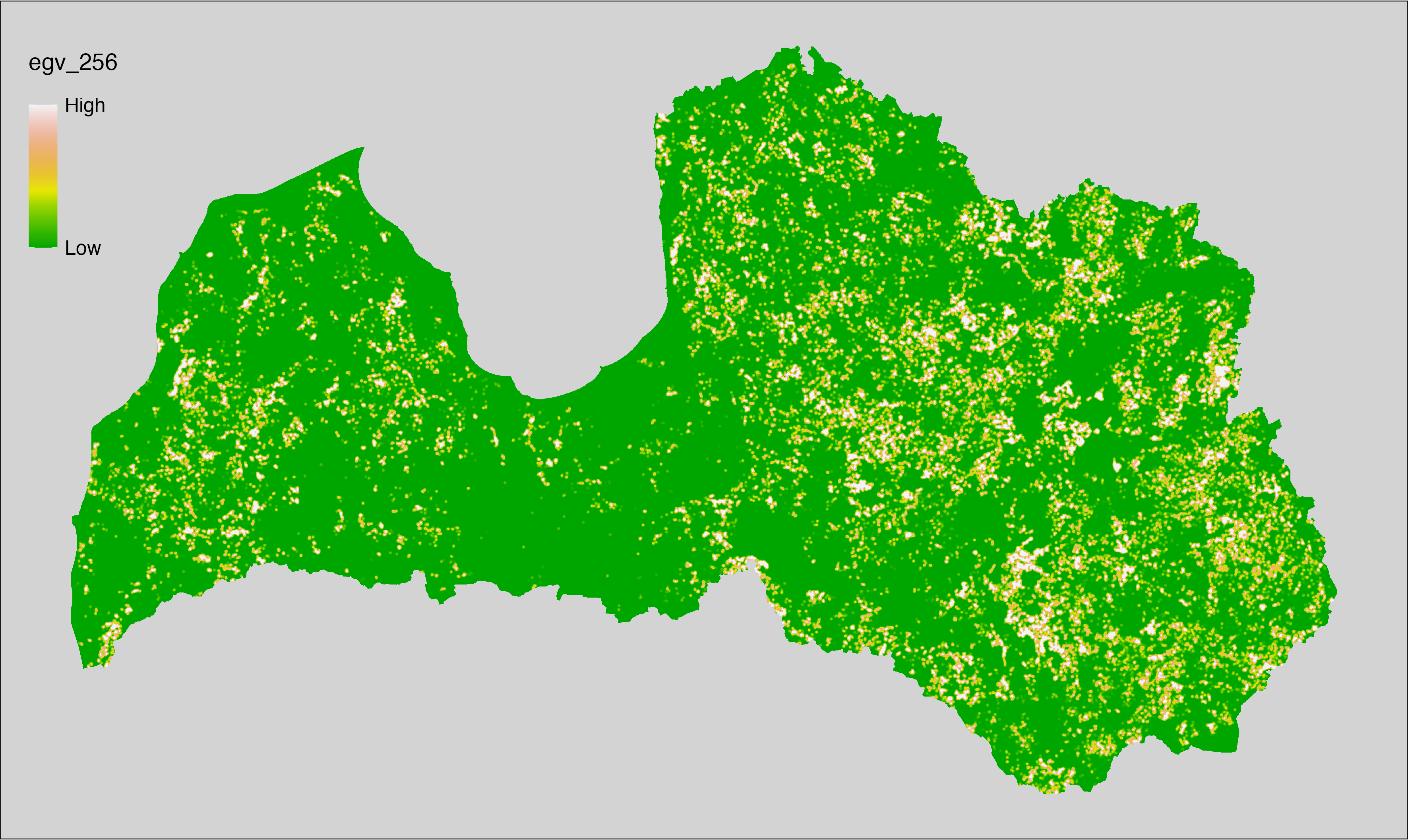
6.257 FarmlandSubsidies_BiologicalSubsidies_r1250
filename: FarmlandSubsidies_BiologicalSubsidies_r1250.tif
layername: egv_257
English name: Fractional cover of Farmland receiving Subsidies for Biological Agriculture within the 1.25 km landscape
Latvian name: Bioloģiskās lauksaimniecības atbalstam pieteikto lauksaimniecības platību īpatsvars 1,25 km ainavā
Procedure: The cover fraction within a radius of 1250 m around the analysis grid cell
is calculated as the area-weighted sum of the analysis cells inside
the buffer, using the workflow egvtools::radius_function(). During the calculation of the landscape
metric, inverse distance weighted (power = 2) gap filling on the output is
applied to ensure no missing values at the edges. Then the layer is
rewritten to set its name. Finally, the layer is standardised by
subtracting the arithmetic mean and dividing by the root mean squared error.
Code
# libs ----
if(!require(terra)) {install.packages("terra"); require(terra)}
if(!require(egvtools)) {remotes::install_github("aavotins/egvtools"); require(egvtools)}
# Templates -----
template100=rast("./Templates/TemplateRasters/LV100m_10km.tif")
# radii ----
radius_function(
kvadrati_path = "./Templates/TemplateGrids/tiles/",
radii_path = "./Templates/TemplateGridPoints/tiles/",
tikls100_path = "./Templates/TemplateGrids/tikls100_sauzeme.parquet",
template_path = "./Templates/TemplateRasters/LV100m_10km.tif",
input_layers = c("./RasterGrids_100m/2024/RAW/FarmlandSubsidies_BiologicalSubsidies_cell.tif"),
layer_prefixes = c("FarmlandSubsidies_BiologicalSubsidies"),
output_dir = "./RasterGrids_100m/2024/RAW/",
n_workers = 6,
radii = c("r1250"),
radius_mode = "sparse",
extract_fun = "mean",
fill_missing = TRUE,
IDW_weight = 2,
future_max_size = 40 * 1024^3)
# FarmlandSubsidies_BiologicalSubsidies_r1250.tif egv_257
slanis=rast("./RasterGrids_100m/2024/RAW/FarmlandSubsidies_BiologicalSubsidies_r1250.tif")
names(slanis)="egv_257"
slanis2=project(slanis,template100)
writeRaster(slanis2,
"./RasterGrids_100m/2024/RAW/FarmlandSubsidies_BiologicalSubsidies_r1250.tif",
overwrite=TRUE)
# standardisation ----
if(!require(terra)) {install.packages("terra"); require(terra)}
if(!require(tidyverse)) {install.packages("tidyverse"); require(tidyverse)}
nosaukums="FarmlandSubsidies_BiologicalSubsidies_r1250.tif"
ielasisanas_cels=paste0("./RasterGrids_100m/2024/RAW/",nosaukums)
saglabasanas_cels=paste0("./RasterGrids_100m/2024/Scaled/",nosaukums)
slanis=rast(ielasisanas_cels)
videjais=global(slanis,fun="mean",na.rm=TRUE)
centrets=slanis-videjais[,1]
standartnovirze=terra::global(centrets,fun="rms",na.rm=TRUE)
merogots=centrets/standartnovirze[,1]
writeRaster(merogots,
filename=saglabasanas_cels,
overwrite=TRUE)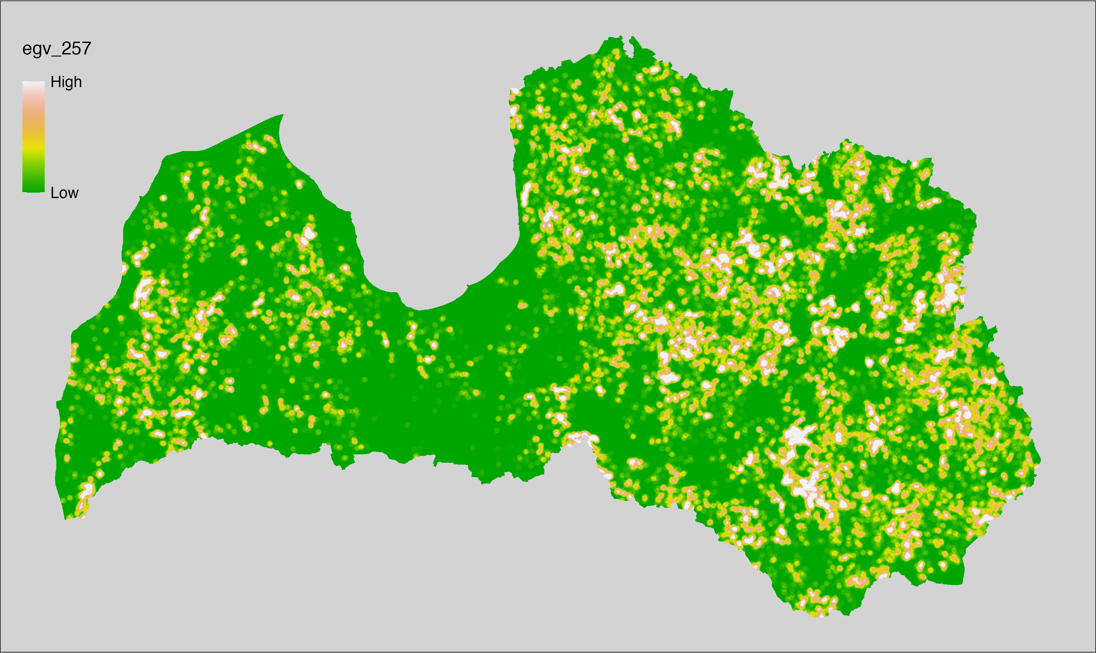
6.258 FarmlandSubsidies_BiologicalSubsidies_r3000
filename: FarmlandSubsidies_BiologicalSubsidies_r3000.tif
layername: egv_258
English name: Fractional cover of Farmland receiving Subsidies for Biological Agriculture within the 3 km landscape
Latvian name: Bioloģiskās lauksaimniecības atbalstam pieteikto lauksaimniecības platību īpatsvars 3 km ainavā
Procedure: The cover fraction within a radius of 3000 m around the analysis grid cell
is calculated as the area-weighted sum of the analysis cells inside
the buffer, using the workflow egvtools::radius_function(). During the calculation of the landscape
metric, inverse distance weighted (power = 2) gap filling on the output is
applied to ensure no missing values at the edges. Then the layer is
rewritten to set its name. Finally, the layer is standardised by
subtracting the arithmetic mean and dividing by the root mean squared error.
Code
# libs ----
if(!require(terra)) {install.packages("terra"); require(terra)}
if(!require(egvtools)) {remotes::install_github("aavotins/egvtools"); require(egvtools)}
# Templates -----
template100=rast("./Templates/TemplateRasters/LV100m_10km.tif")
# radii ----
radius_function(
kvadrati_path = "./Templates/TemplateGrids/tiles/",
radii_path = "./Templates/TemplateGridPoints/tiles/",
tikls100_path = "./Templates/TemplateGrids/tikls100_sauzeme.parquet",
template_path = "./Templates/TemplateRasters/LV100m_10km.tif",
input_layers = c("./RasterGrids_100m/2024/RAW/FarmlandSubsidies_BiologicalSubsidies_cell.tif"),
layer_prefixes = c("FarmlandSubsidies_BiologicalSubsidies"),
output_dir = "./RasterGrids_100m/2024/RAW/",
n_workers = 6,
radii = c("r3000"),
radius_mode = "sparse",
extract_fun = "mean",
fill_missing = TRUE,
IDW_weight = 2,
future_max_size = 40 * 1024^3)
# FarmlandSubsidies_BiologicalSubsidies_r3000.tif egv_258
slanis=rast("./RasterGrids_100m/2024/RAW/FarmlandSubsidies_BiologicalSubsidies_r3000.tif")
names(slanis)="egv_258"
slanis2=project(slanis,template100)
writeRaster(slanis2,
"./RasterGrids_100m/2024/RAW/FarmlandSubsidies_BiologicalSubsidies_r3000.tif",
overwrite=TRUE)
# standardisation ----
if(!require(terra)) {install.packages("terra"); require(terra)}
if(!require(tidyverse)) {install.packages("tidyverse"); require(tidyverse)}
nosaukums="FarmlandSubsidies_BiologicalSubsidies_r3000.tif"
ielasisanas_cels=paste0("./RasterGrids_100m/2024/RAW/",nosaukums)
saglabasanas_cels=paste0("./RasterGrids_100m/2024/Scaled/",nosaukums)
slanis=rast(ielasisanas_cels)
videjais=global(slanis,fun="mean",na.rm=TRUE)
centrets=slanis-videjais[,1]
standartnovirze=terra::global(centrets,fun="rms",na.rm=TRUE)
merogots=centrets/standartnovirze[,1]
writeRaster(merogots,
filename=saglabasanas_cels,
overwrite=TRUE)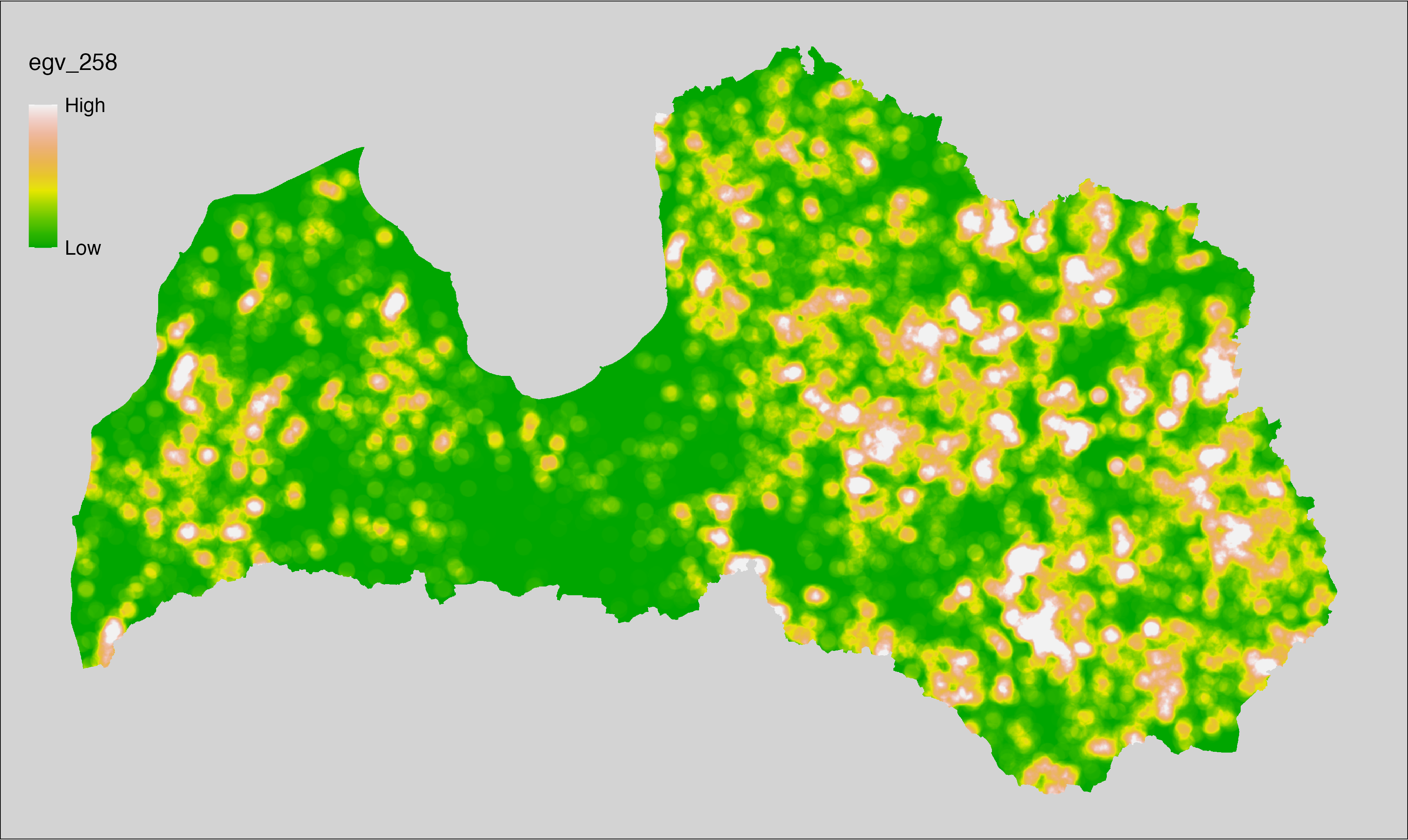
6.259 FarmlandSubsidies_BiologicalSubsidies_r10000
filename: FarmlandSubsidies_BiologicalSubsidies_r10000.tif
layername: egv_259
English name: Fractional cover of Farmland receiving Subsidies for Biological Agriculture within the 10 km landscape
Latvian name: Bioloģiskās lauksaimniecības atbalstam pieteikto lauksaimniecības platību īpatsvars 10 km ainavā
Procedure: The cover fraction within a radius of 10000 m around the analysis grid cell
is calculated as the area-weighted sum of the analysis cells inside
the buffer, using the workflow egvtools::radius_function(). During the calculation of the landscape
metric, inverse distance weighted (power = 2) gap filling on the output is
applied to ensure no missing values at the edges. Then the layer is
rewritten to set its name. Finally, the layer is standardised by
subtracting the arithmetic mean and dividing by the root mean squared error.
Code
# libs ----
if(!require(terra)) {install.packages("terra"); require(terra)}
if(!require(egvtools)) {remotes::install_github("aavotins/egvtools"); require(egvtools)}
# Templates -----
template100=rast("./Templates/TemplateRasters/LV100m_10km.tif")
# radii ----
radius_function(
kvadrati_path = "./Templates/TemplateGrids/tiles/",
radii_path = "./Templates/TemplateGridPoints/tiles/",
tikls100_path = "./Templates/TemplateGrids/tikls100_sauzeme.parquet",
template_path = "./Templates/TemplateRasters/LV100m_10km.tif",
input_layers = c("./RasterGrids_100m/2024/RAW/FarmlandSubsidies_BiologicalSubsidies_cell.tif"),
layer_prefixes = c("FarmlandSubsidies_BiologicalSubsidies"),
output_dir = "./RasterGrids_100m/2024/RAW/",
n_workers = 6,
radii = c("r10000"),
radius_mode = "sparse",
extract_fun = "mean",
fill_missing = TRUE,
IDW_weight = 2,
future_max_size = 40 * 1024^3)
# FarmlandSubsidies_BiologicalSubsidies_r10000.tif egv_259
slanis=rast("./RasterGrids_100m/2024/RAW/FarmlandSubsidies_BiologicalSubsidies_r10000.tif")
names(slanis)="egv_259"
slanis2=project(slanis,template100)
writeRaster(slanis2,
"./RasterGrids_100m/2024/RAW/FarmlandSubsidies_BiologicalSubsidies_r10000.tif",
overwrite=TRUE)
# standardisation ----
if(!require(terra)) {install.packages("terra"); require(terra)}
if(!require(tidyverse)) {install.packages("tidyverse"); require(tidyverse)}
nosaukums="FarmlandSubsidies_BiologicalSubsidies_r10000.tif"
ielasisanas_cels=paste0("./RasterGrids_100m/2024/RAW/",nosaukums)
saglabasanas_cels=paste0("./RasterGrids_100m/2024/Scaled/",nosaukums)
slanis=rast(ielasisanas_cels)
videjais=global(slanis,fun="mean",na.rm=TRUE)
centrets=slanis-videjais[,1]
standartnovirze=terra::global(centrets,fun="rms",na.rm=TRUE)
merogots=centrets/standartnovirze[,1]
writeRaster(merogots,
filename=saglabasanas_cels,
overwrite=TRUE)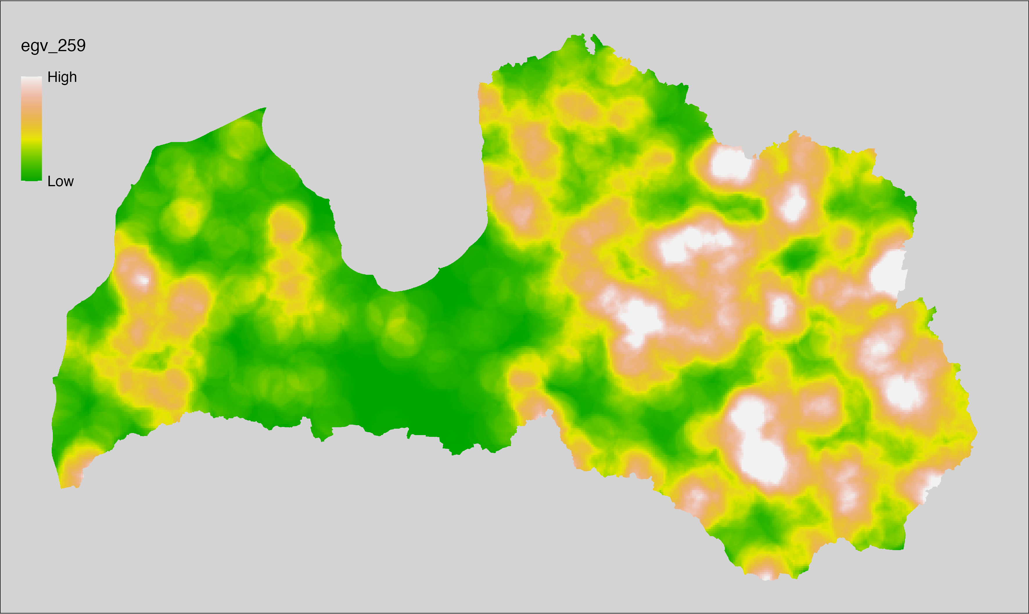
6.260 FarmlandTrees_PermanentCrops_cell
filename: FarmlandTrees_PermanentCrops_cell.tif
layername: egv_260
English name: Fractional cover of Permanent Crops within the analysis cell (1 ha)
Latvian name: Ilggadīgo kultūraugu platības īpatsvars analīzes šūnā (1 ha)
Procedure: First, agricultural parcels declared as permanent crops are
selected from the Rural Support Service’s information on declared
fields. Geometries are then rasterised to input resolution, ensuring
value 1 at the polygon locations and value 0 elsewhere. Rasterisation is
performed using the workflow egvtools::polygon2input(). Once rasterised, the
layer is aggregated to EGV resolution using the workflow egvtools::input2egv(),
which calculates the arithmetic mean and thus
results in a cover fraction. During aggregation, inverse
distance weighted (power = 2) gap filling on the output is applied to
ensure no missing values at the edges. Finally, the layer is standardised
by subtracting the arithmetic mean and dividing by the root mean squared error.
Code
# libs ----
if(!require(egvtools)) {remotes::install_github("aavotins/egvtools"); require(egvtools)}
if(!require(terra)) {install.packages("terra"); require(terra)}
if(!require(sf)) {install.packages("sf"); require(sf)}
if(!require(tidyverse)) {install.packages("tidyverse"); require(tidyverse)}
if(!require(sfarrow)) {install.packages("sfarrow"); require(sfarrow)}
if(!require(readxl)) {install.packages("readxl"); require(readxl)}
if(!require(raster)) {install.packages("raster"); require(raster)}
if(!require(fasterize)) {install.packages("fasterize"); require(fasterize)}
# templates ----
template100=rast("./Templates/TemplateRasters/LV100m_10km.tif")
template10=rast("./Templates/TemplateRasters/LV10m_10km.tif")
rastrs10=raster(template10)
nulls10=rast("./Templates/TemplateRasters/nulls_LV10m_10km.tif")
nulls100=rast("./Templates/TemplateRasters/nulls_LV100m_10km.tif")
# codes ----
kodi=read_excel("./Geodata/2024/LAD/KulturuKodi_2024.xlsx")
kodi$kods=as.character(kodi$kods)
# LAD ----
lad=sfarrow::st_read_parquet("./Geodata/2024/LAD/Lauki_2024.parquet")
lad$yes=1
lad=lad %>%
left_join(kodi,by=c("PRODUCT_CODE"="kods"))
# simple landscape ----
simple_landscape=rast("RasterGrids_10m/2024/Ainava_vienk_mask.tif")
# FarmlandTrees_PermanentCrops_cell.tif egv_260 ----
dati=lad %>%
filter(SDM_grupa_sakums == "augļudārzi")
table(dati$SDM_grupa_sakums,useNA="always")
dati=dati %>%
dplyr::select(yes)
topo=sfarrow::st_read_parquet("./Geodata/2024/TopographicMap/LandusA_COMB.parquet")
dati_topo= topo %>%
filter(FNAME %in% c("poligons_Augludarzs","poligons_Augļudārzs",
"poligons_Ogulājs","poligons_Ogulajs")) %>%
mutate(yes=1) %>%
dplyr::select(yes)
abidati=rbind(dati,dati_topo)
p2i_rez=egvtools::polygon2input(vector_data = abidati,
template_path = "./Templates/TemplateRasters/LV10m_10km.tif",
out_path = "./RasterGrids_10m/2024/",
file_name = "FarmlandTrees_PermanentCrops_input.tif",
value_field = "yes",
prepare=FALSE,
background_raster = "./Templates/TemplateRasters/nulls_LV10m_10km.tif",
plot_result = TRUE)
p2i_rez
i2e_rez=egvtools::input2egv(input=paste0("./RasterGrids_10m/2024/",
"FarmlandTrees_PermanentCrops_input.tif"),
egv_template= "./Templates/TemplateRasters/LV100m_10km.tif",
summary_function = "average",
missing_job = "FillOutput",
outlocation = "./RasterGrids_100m/2024/RAW/",
outfilename = "FarmlandTrees_PermanentCrops_cell.tif",
layername = "egv_260",
idw_weight = 2,
plot_gaps = FALSE,plot_final = TRUE)
i2e_rez
rm(p2i_rez)
rm(i2e_rez)
rm(dati)
rm(topo)
rm(dati_topo)
rm(abidati)
unlink("./RasterGrids_10m/2024/FarmlandTrees_PermanentCrops_input.tif")
# standardisation ----
if(!require(terra)) {install.packages("terra"); require(terra)}
if(!require(tidyverse)) {install.packages("tidyverse"); require(tidyverse)}
nosaukums="FarmlandTrees_PermanentCrops_cell.tif"
ielasisanas_cels=paste0("./RasterGrids_100m/2024/RAW/",nosaukums)
saglabasanas_cels=paste0("./RasterGrids_100m/2024/Scaled/",nosaukums)
slanis=rast(ielasisanas_cels)
videjais=global(slanis,fun="mean",na.rm=TRUE)
centrets=slanis-videjais[,1]
standartnovirze=terra::global(centrets,fun="rms",na.rm=TRUE)
merogots=centrets/standartnovirze[,1]
writeRaster(merogots,
filename=saglabasanas_cels,
overwrite=TRUE)
6.261 FarmlandTrees_PermanentCrops_r500
filename: FarmlandTrees_PermanentCrops_r500.tif
layername: egv_261
English name: Fractional cover of Permanent Crops within the 0.5 km landscape
Latvian name: Ilggadīgo kultūraugu platības īpatsvars 0,5 km ainavā
Procedure: The cover fraction within a radius of 500 m around the analysis grid cell is
calculated as the area-weighted sum of the analysis cells inside the
buffer, using the workflow egvtools::radius_function(). During the calculation of the landscape metric,
inverse distance weighted (power = 2) gap filling on the output is applied
to ensure no missing values at the edges. Then the layer is rewritten to set
its name. Finally, the layer is standardised by subtracting the arithmetic
mean and dividing by the root mean squared error.
Code
# libs ----
if(!require(terra)) {install.packages("terra"); require(terra)}
if(!require(egvtools)) {remotes::install_github("aavotins/egvtools"); require(egvtools)}
# Templates -----
template100=rast("./Templates/TemplateRasters/LV100m_10km.tif")
# radii ----
radius_function(
kvadrati_path = "./Templates/TemplateGrids/tiles/",
radii_path = "./Templates/TemplateGridPoints/tiles/",
tikls100_path = "./Templates/TemplateGrids/tikls100_sauzeme.parquet",
template_path = "./Templates/TemplateRasters/LV100m_10km.tif",
input_layers = c("./RasterGrids_100m/2024/RAW/FarmlandTrees_PermanentCrops_cell.tif"),
layer_prefixes = c("FarmlandTrees_PermanentCrops"),
output_dir = "./RasterGrids_100m/2024/RAW/",
n_workers = 6,
radii = c("r500"),
radius_mode = "sparse",
extract_fun = "mean",
fill_missing = TRUE,
IDW_weight = 2,
future_max_size = 40 * 1024^3)
# FarmlandTrees_PermanentCrops_r500.tif egv_261
slanis=rast("./RasterGrids_100m/2024/RAW/FarmlandTrees_PermanentCrops_r500.tif")
names(slanis)="egv_261"
slanis2=project(slanis,template100)
writeRaster(slanis2,
"./RasterGrids_100m/2024/RAW/FarmlandTrees_PermanentCrops_r500.tif",
overwrite=TRUE)
# standardisation ----
if(!require(terra)) {install.packages("terra"); require(terra)}
if(!require(tidyverse)) {install.packages("tidyverse"); require(tidyverse)}
nosaukums="FarmlandTrees_PermanentCrops_r500.tif"
ielasisanas_cels=paste0("./RasterGrids_100m/2024/RAW/",nosaukums)
saglabasanas_cels=paste0("./RasterGrids_100m/2024/Scaled/",nosaukums)
slanis=rast(ielasisanas_cels)
videjais=global(slanis,fun="mean",na.rm=TRUE)
centrets=slanis-videjais[,1]
standartnovirze=terra::global(centrets,fun="rms",na.rm=TRUE)
merogots=centrets/standartnovirze[,1]
writeRaster(merogots,
filename=saglabasanas_cels,
overwrite=TRUE)
6.262 FarmlandTrees_PermanentCrops_r1250
filename: FarmlandTrees_PermanentCrops_r1250.tif
layername: egv_262
English name: Fractional cover of Permanent Crops within the 1.25 km landscape
Latvian name: Ilggadīgo kultūraugu platības īpatsvars 1,25 km ainavā
Procedure: The cover fraction within a radius of 1250 m around the analysis grid cell
is calculated as the area-weighted sum of the analysis cells inside
the buffer, using the workflow egvtools::radius_function(). During the calculation of the landscape
metric, inverse distance weighted (power = 2) gap filling on the output is
applied to ensure no missing values at the edges. Then the layer is
rewritten to set its name. Finally, the layer is standardised by
subtracting the arithmetic mean and dividing by the root mean squared error.
Code
# libs ----
if(!require(terra)) {install.packages("terra"); require(terra)}
if(!require(egvtools)) {remotes::install_github("aavotins/egvtools"); require(egvtools)}
# Templates -----
template100=rast("./Templates/TemplateRasters/LV100m_10km.tif")
# radii ----
radius_function(
kvadrati_path = "./Templates/TemplateGrids/tiles/",
radii_path = "./Templates/TemplateGridPoints/tiles/",
tikls100_path = "./Templates/TemplateGrids/tikls100_sauzeme.parquet",
template_path = "./Templates/TemplateRasters/LV100m_10km.tif",
input_layers = c("./RasterGrids_100m/2024/RAW/FarmlandTrees_PermanentCrops_cell.tif"),
layer_prefixes = c("FarmlandTrees_PermanentCrops"),
output_dir = "./RasterGrids_100m/2024/RAW/",
n_workers = 6,
radii = c("r1250"),
radius_mode = "sparse",
extract_fun = "mean",
fill_missing = TRUE,
IDW_weight = 2,
future_max_size = 40 * 1024^3)
# FarmlandTrees_PermanentCrops_r1250.tif egv_262
slanis=rast("./RasterGrids_100m/2024/RAW/FarmlandTrees_PermanentCrops_r1250.tif")
names(slanis)="egv_262"
slanis2=project(slanis,template100)
writeRaster(slanis2,
"./RasterGrids_100m/2024/RAW/FarmlandTrees_PermanentCrops_r1250.tif",
overwrite=TRUE)
# standardisation ----
if(!require(terra)) {install.packages("terra"); require(terra)}
if(!require(tidyverse)) {install.packages("tidyverse"); require(tidyverse)}
nosaukums="FarmlandTrees_PermanentCrops_r1250.tif"
ielasisanas_cels=paste0("./RasterGrids_100m/2024/RAW/",nosaukums)
saglabasanas_cels=paste0("./RasterGrids_100m/2024/Scaled/",nosaukums)
slanis=rast(ielasisanas_cels)
videjais=global(slanis,fun="mean",na.rm=TRUE)
centrets=slanis-videjais[,1]
standartnovirze=terra::global(centrets,fun="rms",na.rm=TRUE)
merogots=centrets/standartnovirze[,1]
writeRaster(merogots,
filename=saglabasanas_cels,
overwrite=TRUE)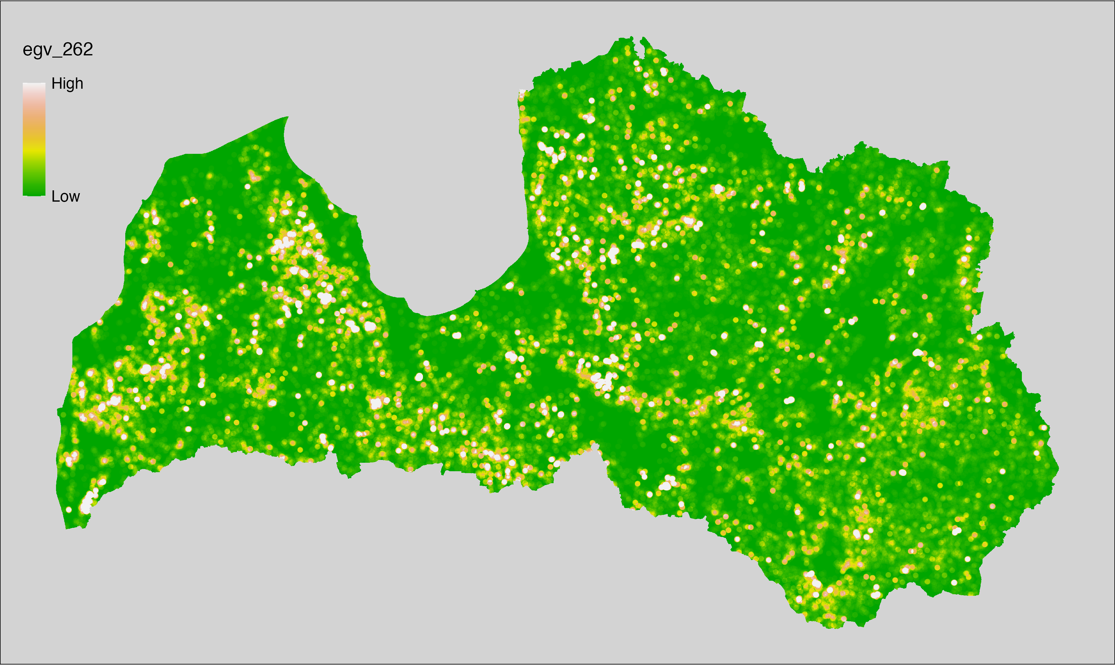
6.263 FarmlandTrees_PermanentCrops_r3000
filename: FarmlandTrees_PermanentCrops_r3000.tif
layername: egv_263
English name: Fractional cover of Permanent Crops within the 3 km landscape
Latvian name: Ilggadīgo kultūraugu platības īpatsvars 3 km ainavā
Procedure: The cover fraction within a radius of 3000 m around the analysis grid cell
is calculated as the area-weighted sum of the analysis cells inside
the buffer, using the workflow egvtools::radius_function(). During the calculation of the landscape
metric, inverse distance weighted (power = 2) gap filling on the output is
applied to ensure no missing values at the edges. Then the layer is
rewritten to set its name. Finally, the layer is standardised by
subtracting the arithmetic mean and dividing by the root mean squared error.
Code
# libs ----
if(!require(terra)) {install.packages("terra"); require(terra)}
if(!require(egvtools)) {remotes::install_github("aavotins/egvtools"); require(egvtools)}
# Templates -----
template100=rast("./Templates/TemplateRasters/LV100m_10km.tif")
# radii ----
radius_function(
kvadrati_path = "./Templates/TemplateGrids/tiles/",
radii_path = "./Templates/TemplateGridPoints/tiles/",
tikls100_path = "./Templates/TemplateGrids/tikls100_sauzeme.parquet",
template_path = "./Templates/TemplateRasters/LV100m_10km.tif",
input_layers = c("./RasterGrids_100m/2024/RAW/FarmlandTrees_PermanentCrops_cell.tif"),
layer_prefixes = c("FarmlandTrees_PermanentCrops"),
output_dir = "./RasterGrids_100m/2024/RAW/",
n_workers = 6,
radii = c("r3000"),
radius_mode = "sparse",
extract_fun = "mean",
fill_missing = TRUE,
IDW_weight = 2,
future_max_size = 40 * 1024^3)
# FarmlandTrees_PermanentCrops_r3000.tif egv_263
slanis=rast("./RasterGrids_100m/2024/RAW/FarmlandTrees_PermanentCrops_r3000.tif")
names(slanis)="egv_263"
slanis2=project(slanis,template100)
writeRaster(slanis2,
"./RasterGrids_100m/2024/RAW/FarmlandTrees_PermanentCrops_r3000.tif",
overwrite=TRUE)
# standardisation ----
if(!require(terra)) {install.packages("terra"); require(terra)}
if(!require(tidyverse)) {install.packages("tidyverse"); require(tidyverse)}
nosaukums="FarmlandTrees_PermanentCrops_r3000.tif"
ielasisanas_cels=paste0("./RasterGrids_100m/2024/RAW/",nosaukums)
saglabasanas_cels=paste0("./RasterGrids_100m/2024/Scaled/",nosaukums)
slanis=rast(ielasisanas_cels)
videjais=global(slanis,fun="mean",na.rm=TRUE)
centrets=slanis-videjais[,1]
standartnovirze=terra::global(centrets,fun="rms",na.rm=TRUE)
merogots=centrets/standartnovirze[,1]
writeRaster(merogots,
filename=saglabasanas_cels,
overwrite=TRUE)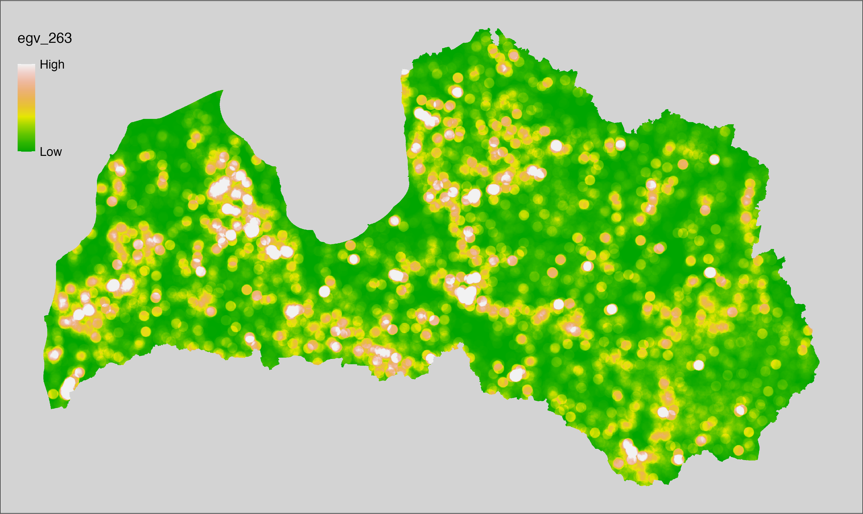
6.264 FarmlandTrees_PermanentCrops_r10000
filename: FarmlandTrees_PermanentCrops_r10000.tif
layername: egv_264
English name: Fractional cover of Permanent Crops within the 10 km landscape
Latvian name: Ilggadīgo kultūraugu platības īpatsvars 10 km ainavā
Procedure: The cover fraction within a radius of 10000 m around the analysis grid cell
is calculated as the area-weighted sum of the analysis cells inside
the buffer, using the workflow egvtools::radius_function(). During the calculation of the landscape
metric, inverse distance weighted (power = 2) gap filling on the output is
applied to ensure no missing values at the edges. Then the layer is
rewritten to set its name. Finally, the layer is standardised by
subtracting the arithmetic mean and dividing by the root mean squared error.
Code
# libs ----
if(!require(terra)) {install.packages("terra"); require(terra)}
if(!require(egvtools)) {remotes::install_github("aavotins/egvtools"); require(egvtools)}
# Templates -----
template100=rast("./Templates/TemplateRasters/LV100m_10km.tif")
# radii ----
radius_function(
kvadrati_path = "./Templates/TemplateGrids/tiles/",
radii_path = "./Templates/TemplateGridPoints/tiles/",
tikls100_path = "./Templates/TemplateGrids/tikls100_sauzeme.parquet",
template_path = "./Templates/TemplateRasters/LV100m_10km.tif",
input_layers = c("./RasterGrids_100m/2024/RAW/FarmlandTrees_PermanentCrops_cell.tif"),
layer_prefixes = c("FarmlandTrees_PermanentCrops"),
output_dir = "./RasterGrids_100m/2024/RAW/",
n_workers = 6,
radii = c("r10000"),
radius_mode = "sparse",
extract_fun = "mean",
fill_missing = TRUE,
IDW_weight = 2,
future_max_size = 40 * 1024^3)
# FarmlandTrees_PermanentCrops_r10000.tif egv_264
slanis=rast("./RasterGrids_100m/2024/RAW/FarmlandTrees_PermanentCrops_r10000.tif")
names(slanis)="egv_264"
slanis2=project(slanis,template100)
writeRaster(slanis2,
"./RasterGrids_100m/2024/RAW/FarmlandTrees_PermanentCrops_r10000.tif",
overwrite=TRUE)
# standardisation ----
if(!require(terra)) {install.packages("terra"); require(terra)}
if(!require(tidyverse)) {install.packages("tidyverse"); require(tidyverse)}
nosaukums="FarmlandTrees_PermanentCrops_r10000.tif"
ielasisanas_cels=paste0("./RasterGrids_100m/2024/RAW/",nosaukums)
saglabasanas_cels=paste0("./RasterGrids_100m/2024/Scaled/",nosaukums)
slanis=rast(ielasisanas_cels)
videjais=global(slanis,fun="mean",na.rm=TRUE)
centrets=slanis-videjais[,1]
standartnovirze=terra::global(centrets,fun="rms",na.rm=TRUE)
merogots=centrets/standartnovirze[,1]
writeRaster(merogots,
filename=saglabasanas_cels,
overwrite=TRUE)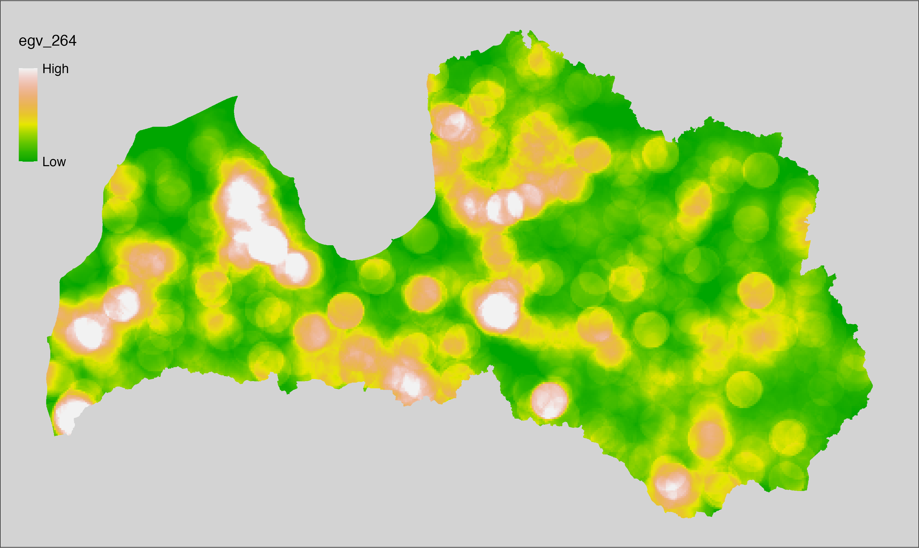
6.265 FarmlandTrees_ShortRotationCoppice_cell
filename: FarmlandTrees_ShortRotationCoppice_cell.tif
layername: egv_265
English name: Fractional cover of Short-rotation Coppice and Other Woody Energy Crops within the analysis cell (1 ha)
Latvian name: Īscirtmeta atvasāju un enerģijai audzētu kokaugu platības īpatsvars analīzes šūnā (1 ha)
Procedure: First, agricultural parcels declared as short rotation coppice
are selected from the Rural Support Service’s information on declared
fields. Geometries are then rasterised to input resolution, ensuring
value 1 at the polygon locations and value 0 elsewhere. Rasterisation is
performed using the workflow egvtools::polygon2input(). Once rasterised, the
layer is aggregated to EGV resolution using the workflow egvtools::input2egv(),
which calculates the arithmetic mean and thus
results in a cover fraction. During aggregation, inverse
distance weighted (power = 2) gap filling on the output is applied to
ensure no missing values at the edges. Finally, the layer is standardised
by subtracting the arithmetic mean and dividing by the root mean squared error.
Code
# libs ----
if(!require(egvtools)) {remotes::install_github("aavotins/egvtools"); require(egvtools)}
if(!require(terra)) {install.packages("terra"); require(terra)}
if(!require(sf)) {install.packages("sf"); require(sf)}
if(!require(tidyverse)) {install.packages("tidyverse"); require(tidyverse)}
if(!require(sfarrow)) {install.packages("sfarrow"); require(sfarrow)}
if(!require(readxl)) {install.packages("readxl"); require(readxl)}
if(!require(raster)) {install.packages("raster"); require(raster)}
if(!require(fasterize)) {install.packages("fasterize"); require(fasterize)}
# templates ----
template100=rast("./Templates/TemplateRasters/LV100m_10km.tif")
template10=rast("./Templates/TemplateRasters/LV10m_10km.tif")
rastrs10=raster(template10)
nulls10=rast("./Templates/TemplateRasters/nulls_LV10m_10km.tif")
nulls100=rast("./Templates/TemplateRasters/nulls_LV100m_10km.tif")
# codes ----
kodi=read_excel("./Geodata/2024/LAD/KulturuKodi_2024.xlsx")
kodi$kods=as.character(kodi$kods)
# LAD ----
lad=sfarrow::st_read_parquet("./Geodata/2024/LAD/Lauki_2024.parquet")
lad$yes=1
lad=lad %>%
left_join(kodi,by=c("PRODUCT_CODE"="kods"))
# simple landscape ----
simple_landscape=rast("RasterGrids_10m/2024/Ainava_vienk_mask.tif")
# FarmlandTrees_ShortRotationCoppice_cell.tif egv_265 ----
dati=lad %>%
filter(SDM_grupa_sakums == "krūmveida ilggadīgie stādījumi")
table(dati$SDM_grupa_sakums,useNA="always")
p2i_rez=egvtools::polygon2input(vector_data = dati,
template_path = "./Templates/TemplateRasters/LV10m_10km.tif",
out_path = "./RasterGrids_10m/2024/",
file_name = "FarmlandTrees_ShortRotationCoppice_input.tif",
value_field = "yes",
prepare=FALSE,
background_raster = "./Templates/TemplateRasters/nulls_LV10m_10km.tif",
plot_result = TRUE)
p2i_rez
i2e_rez=egvtools::input2egv(input=paste0("./RasterGrids_10m/2024/",
"FarmlandTrees_ShortRotationCoppice_input.tif"),
egv_template= "./Templates/TemplateRasters/LV100m_10km.tif",
summary_function = "average",
missing_job = "FillOutput",
outlocation = "./RasterGrids_100m/2024/RAW/",
outfilename = "FarmlandTrees_ShortRotationCoppice_cell.tif",
layername = "egv_265",
idw_weight = 2,
plot_gaps = FALSE,plot_final = TRUE)
i2e_rez
rm(p2i_rez)
rm(i2e_rez)
rm(dati)
unlink("./RasterGrids_10m/2024/FarmlandTrees_ShortRotationCoppice_input.tif")
# standardisation ----
if(!require(terra)) {install.packages("terra"); require(terra)}
if(!require(tidyverse)) {install.packages("tidyverse"); require(tidyverse)}
nosaukums="FarmlandTrees_ShortRotationCoppice_cell.tif"
ielasisanas_cels=paste0("./RasterGrids_100m/2024/RAW/",nosaukums)
saglabasanas_cels=paste0("./RasterGrids_100m/2024/Scaled/",nosaukums)
slanis=rast(ielasisanas_cels)
videjais=global(slanis,fun="mean",na.rm=TRUE)
centrets=slanis-videjais[,1]
standartnovirze=terra::global(centrets,fun="rms",na.rm=TRUE)
merogots=centrets/standartnovirze[,1]
writeRaster(merogots,
filename=saglabasanas_cels,
overwrite=TRUE)
6.266 FarmlandTrees_ShortRotationCoppice_r500
filename: FarmlandTrees_ShortRotationCoppice_r500.tif
layername: egv_266
English name: Fractional cover of Short-rotation Coppice and Other Woody Energy Crops within the 0.5 km landscape
Latvian name: Īscirtmeta atvasāju un enerģijai audzētu kokaugu platības īpatsvars 0,5 km ainavā
Procedure: The cover fraction within a radius of 500 m around the analysis grid cell is
calculated as the area-weighted sum of the analysis cells inside the
buffer, using the workflow egvtools::radius_function(). During the calculation of the landscape metric,
inverse distance weighted (power = 2) gap filling on the output is applied
to ensure no missing values at the edges. Then the layer is rewritten to set
its name. Finally, the layer is standardised by subtracting the arithmetic
mean and dividing by the root mean squared error.
Code
# libs ----
if(!require(terra)) {install.packages("terra"); require(terra)}
if(!require(egvtools)) {remotes::install_github("aavotins/egvtools"); require(egvtools)}
# Templates -----
template100=rast("./Templates/TemplateRasters/LV100m_10km.tif")
# radii ----
radius_function(
kvadrati_path = "./Templates/TemplateGrids/tiles/",
radii_path = "./Templates/TemplateGridPoints/tiles/",
tikls100_path = "./Templates/TemplateGrids/tikls100_sauzeme.parquet",
template_path = "./Templates/TemplateRasters/LV100m_10km.tif",
input_layers = c("./RasterGrids_100m/2024/RAW/FarmlandTrees_ShortRotationCoppice_cell.tif"),
layer_prefixes = c("FarmlandTrees_ShortRotationCoppice"),
output_dir = "./RasterGrids_100m/2024/RAW/",
n_workers = 6,
radii = c("r500"),
radius_mode = "sparse",
extract_fun = "mean",
fill_missing = TRUE,
IDW_weight = 2,
future_max_size = 40 * 1024^3)
# FarmlandTrees_ShortRotationCoppice_r500.tif egv_266
slanis=rast("./RasterGrids_100m/2024/RAW/FarmlandTrees_ShortRotationCoppice_r500.tif")
names(slanis)="egv_266"
slanis2=project(slanis,template100)
writeRaster(slanis2,
"./RasterGrids_100m/2024/RAW/FarmlandTrees_ShortRotationCoppice_r500.tif",
overwrite=TRUE)
# standardisation ----
if(!require(terra)) {install.packages("terra"); require(terra)}
if(!require(tidyverse)) {install.packages("tidyverse"); require(tidyverse)}
nosaukums="FarmlandTrees_ShortRotationCoppice_r500.tif"
ielasisanas_cels=paste0("./RasterGrids_100m/2024/RAW/",nosaukums)
saglabasanas_cels=paste0("./RasterGrids_100m/2024/Scaled/",nosaukums)
slanis=rast(ielasisanas_cels)
videjais=global(slanis,fun="mean",na.rm=TRUE)
centrets=slanis-videjais[,1]
standartnovirze=terra::global(centrets,fun="rms",na.rm=TRUE)
merogots=centrets/standartnovirze[,1]
writeRaster(merogots,
filename=saglabasanas_cels,
overwrite=TRUE)
6.267 FarmlandTrees_ShortRotationCoppice_r1250
filename: FarmlandTrees_ShortRotationCoppice_r1250.tif
layername: egv_267
English name: Fractional cover of Short-rotation Coppice and Other Woody Energy Crops within the 1.25 km landscape
Latvian name: Īscirtmeta atvasāju un enerģijai audzētu kokaugu platības īpatsvars 1,25 km ainavā
Procedure: The cover fraction within a radius of 1250 m around the analysis grid cell
is calculated as the area-weighted sum of the analysis cells inside
the buffer, using the workflow egvtools::radius_function(). During the calculation of the landscape
metric, inverse distance weighted (power = 2) gap filling on the output is
applied to ensure no missing values at the edges. Then the layer is
rewritten to set its name. Finally, the layer is standardised by
subtracting the arithmetic mean and dividing by the root mean squared error.
Code
# libs ----
if(!require(terra)) {install.packages("terra"); require(terra)}
if(!require(egvtools)) {remotes::install_github("aavotins/egvtools"); require(egvtools)}
# Templates -----
template100=rast("./Templates/TemplateRasters/LV100m_10km.tif")
# radii ----
radius_function(
kvadrati_path = "./Templates/TemplateGrids/tiles/",
radii_path = "./Templates/TemplateGridPoints/tiles/",
tikls100_path = "./Templates/TemplateGrids/tikls100_sauzeme.parquet",
template_path = "./Templates/TemplateRasters/LV100m_10km.tif",
input_layers = c("./RasterGrids_100m/2024/RAW/FarmlandTrees_ShortRotationCoppice_cell.tif"),
layer_prefixes = c("FarmlandTrees_ShortRotationCoppice"),
output_dir = "./RasterGrids_100m/2024/RAW/",
n_workers = 6,
radii = c("r1250"),
radius_mode = "sparse",
extract_fun = "mean",
fill_missing = TRUE,
IDW_weight = 2,
future_max_size = 40 * 1024^3)
# FarmlandTrees_ShortRotationCoppice_r1250.tif egv_267
slanis=rast("./RasterGrids_100m/2024/RAW/FarmlandTrees_ShortRotationCoppice_r1250.tif")
names(slanis)="egv_267"
slanis2=project(slanis,template100)
writeRaster(slanis2,
"./RasterGrids_100m/2024/RAW/FarmlandTrees_ShortRotationCoppice_r1250.tif",
overwrite=TRUE)
# standardisation ----
if(!require(terra)) {install.packages("terra"); require(terra)}
if(!require(tidyverse)) {install.packages("tidyverse"); require(tidyverse)}
nosaukums="FarmlandTrees_ShortRotationCoppice_r1250.tif"
ielasisanas_cels=paste0("./RasterGrids_100m/2024/RAW/",nosaukums)
saglabasanas_cels=paste0("./RasterGrids_100m/2024/Scaled/",nosaukums)
slanis=rast(ielasisanas_cels)
videjais=global(slanis,fun="mean",na.rm=TRUE)
centrets=slanis-videjais[,1]
standartnovirze=terra::global(centrets,fun="rms",na.rm=TRUE)
merogots=centrets/standartnovirze[,1]
writeRaster(merogots,
filename=saglabasanas_cels,
overwrite=TRUE)
6.268 FarmlandTrees_ShortRotationCoppice_r3000
filename: FarmlandTrees_ShortRotationCoppice_r3000.tif
layername: egv_268
English name: Fractional cover of Short-rotation Coppice and Other Woody Energy Crops within the 3 km landscape
Latvian name: Īscirtmeta atvasāju un enerģijai audzētu kokaugu platības īpatsvars 3 km ainavā
Procedure: The cover fraction within a radius of 3000 m around the analysis grid cell
is calculated as the area-weighted sum of the analysis cells inside
the buffer, using the workflow egvtools::radius_function(). During the calculation of the landscape
metric, inverse distance weighted (power = 2) gap filling on the output is
applied to ensure no missing values at the edges. Then the layer is
rewritten to set its name. Finally, the layer is standardised by
subtracting the arithmetic mean and dividing by the root mean squared error.
Code
# libs ----
if(!require(terra)) {install.packages("terra"); require(terra)}
if(!require(egvtools)) {remotes::install_github("aavotins/egvtools"); require(egvtools)}
# Templates -----
template100=rast("./Templates/TemplateRasters/LV100m_10km.tif")
# radii ----
radius_function(
kvadrati_path = "./Templates/TemplateGrids/tiles/",
radii_path = "./Templates/TemplateGridPoints/tiles/",
tikls100_path = "./Templates/TemplateGrids/tikls100_sauzeme.parquet",
template_path = "./Templates/TemplateRasters/LV100m_10km.tif",
input_layers = c("./RasterGrids_100m/2024/RAW/FarmlandTrees_ShortRotationCoppice_cell.tif"),
layer_prefixes = c("FarmlandTrees_ShortRotationCoppice"),
output_dir = "./RasterGrids_100m/2024/RAW/",
n_workers = 6,
radii = c("r3000"),
radius_mode = "sparse",
extract_fun = "mean",
fill_missing = TRUE,
IDW_weight = 2,
future_max_size = 40 * 1024^3)
# FarmlandTrees_ShortRotationCoppice_r3000.tif egv_268
slanis=rast("./RasterGrids_100m/2024/RAW/FarmlandTrees_ShortRotationCoppice_r3000.tif")
names(slanis)="egv_268"
slanis2=project(slanis,template100)
writeRaster(slanis2,
"./RasterGrids_100m/2024/RAW/FarmlandTrees_ShortRotationCoppice_r3000.tif",
overwrite=TRUE)
# standardisation ----
if(!require(terra)) {install.packages("terra"); require(terra)}
if(!require(tidyverse)) {install.packages("tidyverse"); require(tidyverse)}
nosaukums="FarmlandTrees_ShortRotationCoppice_r3000.tif"
ielasisanas_cels=paste0("./RasterGrids_100m/2024/RAW/",nosaukums)
saglabasanas_cels=paste0("./RasterGrids_100m/2024/Scaled/",nosaukums)
slanis=rast(ielasisanas_cels)
videjais=global(slanis,fun="mean",na.rm=TRUE)
centrets=slanis-videjais[,1]
standartnovirze=terra::global(centrets,fun="rms",na.rm=TRUE)
merogots=centrets/standartnovirze[,1]
writeRaster(merogots,
filename=saglabasanas_cels,
overwrite=TRUE)
6.269 FarmlandTrees_ShortRotationCoppice_r10000
filename: FarmlandTrees_ShortRotationCoppice_r10000.tif
layername: egv_269
English name: Fractional cover of Short-rotation Coppice and Other Woody Energy Crops within the 10 km landscape
Latvian name: Īscirtmeta atvasāju un enerģijai audzētu kokaugu platības īpatsvars 10 km ainavā
Procedure: The cover fraction within a radius of 10000 m around the analysis grid cell
is calculated as the area-weighted sum of the analysis cells inside
the buffer, using the workflow egvtools::radius_function(). During the calculation of the landscape
metric, inverse distance weighted (power = 2) gap filling on the output is
applied to ensure no missing values at the edges. Then the layer is
rewritten to set its name. Finally, the layer is standardised by
subtracting the arithmetic mean and dividing by the root mean squared error.
Code
# libs ----
if(!require(terra)) {install.packages("terra"); require(terra)}
if(!require(egvtools)) {remotes::install_github("aavotins/egvtools"); require(egvtools)}
# Templates -----
template100=rast("./Templates/TemplateRasters/LV100m_10km.tif")
# radii ----
radius_function(
kvadrati_path = "./Templates/TemplateGrids/tiles/",
radii_path = "./Templates/TemplateGridPoints/tiles/",
tikls100_path = "./Templates/TemplateGrids/tikls100_sauzeme.parquet",
template_path = "./Templates/TemplateRasters/LV100m_10km.tif",
input_layers = c("./RasterGrids_100m/2024/RAW/FarmlandTrees_ShortRotationCoppice_cell.tif"),
layer_prefixes = c("FarmlandTrees_ShortRotationCoppice"),
output_dir = "./RasterGrids_100m/2024/RAW/",
n_workers = 6,
radii = c("r10000"),
radius_mode = "sparse",
extract_fun = "mean",
fill_missing = TRUE,
IDW_weight = 2,
future_max_size = 40 * 1024^3)
# FarmlandTrees_ShortRotationCoppice_r10000.tif egv_269
slanis=rast("./RasterGrids_100m/2024/RAW/FarmlandTrees_ShortRotationCoppice_r10000.tif")
names(slanis)="egv_269"
slanis2=project(slanis,template100)
writeRaster(slanis2,
"./RasterGrids_100m/2024/RAW/FarmlandTrees_ShortRotationCoppice_r10000.tif",
overwrite=TRUE)
# standardisation ----
if(!require(terra)) {install.packages("terra"); require(terra)}
if(!require(tidyverse)) {install.packages("tidyverse"); require(tidyverse)}
nosaukums="FarmlandTrees_ShortRotationCoppice_r10000.tif"
ielasisanas_cels=paste0("./RasterGrids_100m/2024/RAW/",nosaukums)
saglabasanas_cels=paste0("./RasterGrids_100m/2024/Scaled/",nosaukums)
slanis=rast(ielasisanas_cels)
videjais=global(slanis,fun="mean",na.rm=TRUE)
centrets=slanis-videjais[,1]
standartnovirze=terra::global(centrets,fun="rms",na.rm=TRUE)
merogots=centrets/standartnovirze[,1]
writeRaster(merogots,
filename=saglabasanas_cels,
overwrite=TRUE)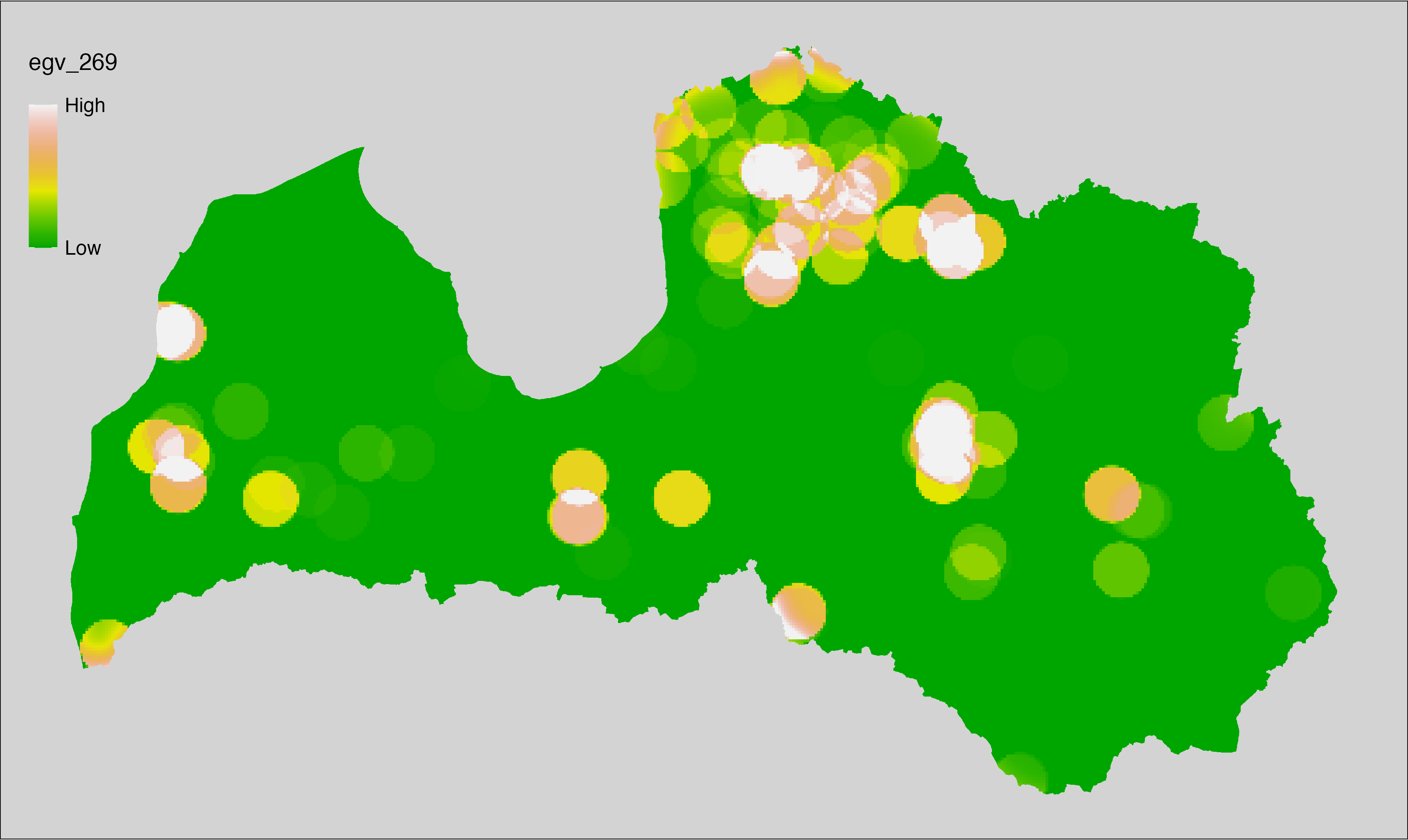
6.270 ForestsAge_ClearcutsLowStands_cell
filename: ForestsAge_ClearcutsLowStands_cell.tif
layername: egv_270
English name: Fractional cover of Clearcuts and Forest Stands lower than 5 m within the analysis cell (1 ha)
Latvian name: Izcirtumu un mežaudžu līdz 5 m augstumam platības īpatsvars analīzes šūnā (1 ha)
Procedure: To prepare this
EGV, stands in land category 10 with a height of less than 5 m are selected from the State
Forest Service’s State Forest Registry and rasterised. After
rasterisation, this layer is covered by a clearcut mask. The resulting layer
is then aggregated to EGV resolution using the workflow egvtools::input2egv(), which
calculates the arithmetic mean to determine the cover fraction. During
aggregation, inverse distance weighted (power = 2) gap filling on the output is
applied to ensure no missing values at the edges. Finally, the layer is
standardised by subtracting the arithmetic mean and dividing by the root mean squared
error.
Code
# libs ----
if(!require(egvtools)) {remotes::install_github("aavotins/egvtools"); require(egvtools)}
if(!require(terra)) {install.packages("terra"); require(terra)}
if(!require(sf)) {install.packages("sf"); require(sf)}
if(!require(tidyverse)) {install.packages("tidyverse"); require(tidyverse)}
if(!require(sfarrow)) {install.packages("sfarrow"); require(sfarrow)}
if(!require(readxl)) {install.packages("readxl"); require(readxl)}
if(!require(raster)) {install.packages("raster"); require(raster)}
if(!require(fasterize)) {install.packages("fasterize"); require(fasterize)}
# templates ----
template100=rast("./Templates/TemplateRasters/LV100m_10km.tif")
template10=rast("./Templates/TemplateRasters/LV10m_10km.tif")
rastrs10=raster(template10)
nulls10=rast("./Templates/TemplateRasters/nulls_LV10m_10km.tif")
nulls100=rast("./Templates/TemplateRasters/nulls_LV100m_10km.tif")
# simple landscape ----
simple_landscape=rast("RasterGrids_10m/2024/Ainava_vienk_mask.tif")
# mvr ----
mvr=st_read_parquet("./Geodata/2024/MVR/nogabali_2024janv.parquet")
mvr$yes=1
# ForestsAge_ClearcutsLowStands_cell.tif egv_270 ----
zemas_audzes=mvr %>%
filter(zkat=="10") %>%
filter(h10<5) %>%
dplyr::select(yes)
r_zemasaudzes=fasterize(zemas_audzes,rastrs10,field="yes")
t_zemasaudzes=rast(r_zemasaudzes)
plot(t_zemasaudzes)
cleacuts_low=cover(t_zemasaudzes,clearcut_mask)
plot(cleacuts_low)
i2e_rez=egvtools::input2egv(input=cleacuts_low,
egv_template= "./Templates/TemplateRasters/LV100m_10km.tif",
summary_function = "average",
missing_job = "FillOutput",
outlocation = "./RasterGrids_100m/2024/RAW/",
outfilename = "ForestsAge_ClearcutsLowStands_cell.tif",
layername = "egv_270",
idw_weight = 2,
plot_gaps = FALSE,plot_final = TRUE)
i2e_rez
rm(i2e_rez)
rm(zemas_audzes)
rm(r_zemasaudzes)
rm(t_zemasaudzes)
rm(cleacuts_low)
# standardisation ----
if(!require(terra)) {install.packages("terra"); require(terra)}
if(!require(tidyverse)) {install.packages("tidyverse"); require(tidyverse)}
nosaukums="ForestsAge_ClearcutsLowStands_cell.tif"
ielasisanas_cels=paste0("./RasterGrids_100m/2024/RAW/",nosaukums)
saglabasanas_cels=paste0("./RasterGrids_100m/2024/Scaled/",nosaukums)
slanis=rast(ielasisanas_cels)
videjais=global(slanis,fun="mean",na.rm=TRUE)
centrets=slanis-videjais[,1]
standartnovirze=terra::global(centrets,fun="rms",na.rm=TRUE)
merogots=centrets/standartnovirze[,1]
writeRaster(merogots,
filename=saglabasanas_cels,
overwrite=TRUE)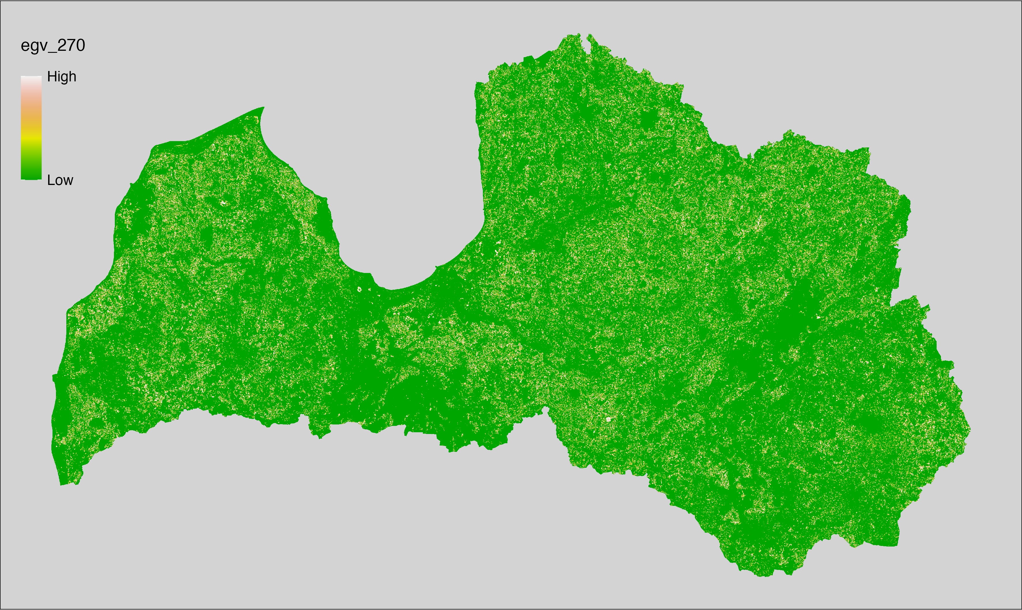
6.271 ForestsAge_ClearcutsLowStands_r500
filename: ForestsAge_ClearcutsLowStands_r500.tif
layername: egv_271
English name: Fractional cover of Clearcuts and Forest Stands lower than 5 m within the 0.5 km landscape
Latvian name: Izcirtumu un mežaudžu līdz 5 m augstumam platības īpatsvars 0,5 km ainavā
Procedure: The cover fraction within a radius of 500 m around the analysis grid cell is
calculated as the area-weighted sum of the analysis cells inside the
buffer, using the workflow egvtools::radius_function(). During the calculation of the landscape metric,
inverse distance weighted (power = 2) gap filling on the output is applied
to ensure no missing values at the edges. Then the layer is rewritten to set
its name. Finally, the layer is standardised by subtracting the arithmetic
mean and dividing by the root mean squared error.
Code
# libs ----
if(!require(terra)) {install.packages("terra"); require(terra)}
if(!require(egvtools)) {remotes::install_github("aavotins/egvtools"); require(egvtools)}
# Templates -----
template100=rast("./Templates/TemplateRasters/LV100m_10km.tif")
# radii ----
radius_function(
kvadrati_path = "./Templates/TemplateGrids/tiles/",
radii_path = "./Templates/TemplateGridPoints/tiles/",
tikls100_path = "./Templates/TemplateGrids/tikls100_sauzeme.parquet",
template_path = "./Templates/TemplateRasters/LV100m_10km.tif",
input_layers = c("./RasterGrids_100m/2024/RAW/ForestsAge_ClearcutsLowStands_cell.tif"),
layer_prefixes = c("ForestsAge_ClearcutsLowStands"),
output_dir = "./RasterGrids_100m/2024/RAW/",
n_workers = 6,
radii = c("r500"),
radius_mode = "sparse",
extract_fun = "mean",
fill_missing = TRUE,
IDW_weight = 2,
future_max_size = 40 * 1024^3)
# ForestsAge_ClearcutsLowStands_r500.tif egv_271
slanis=rast("./RasterGrids_100m/2024/RAW/ForestsAge_ClearcutsLowStands_r500.tif")
names(slanis)="egv_271"
slanis2=project(slanis,template100)
writeRaster(slanis2,
"./RasterGrids_100m/2024/RAW/ForestsAge_ClearcutsLowStands_r500.tif",
overwrite=TRUE)
# standardisation ----
if(!require(terra)) {install.packages("terra"); require(terra)}
if(!require(tidyverse)) {install.packages("tidyverse"); require(tidyverse)}
nosaukums="ForestsAge_ClearcutsLowStands_r500.tif"
ielasisanas_cels=paste0("./RasterGrids_100m/2024/RAW/",nosaukums)
saglabasanas_cels=paste0("./RasterGrids_100m/2024/Scaled/",nosaukums)
slanis=rast(ielasisanas_cels)
videjais=global(slanis,fun="mean",na.rm=TRUE)
centrets=slanis-videjais[,1]
standartnovirze=terra::global(centrets,fun="rms",na.rm=TRUE)
merogots=centrets/standartnovirze[,1]
writeRaster(merogots,
filename=saglabasanas_cels,
overwrite=TRUE)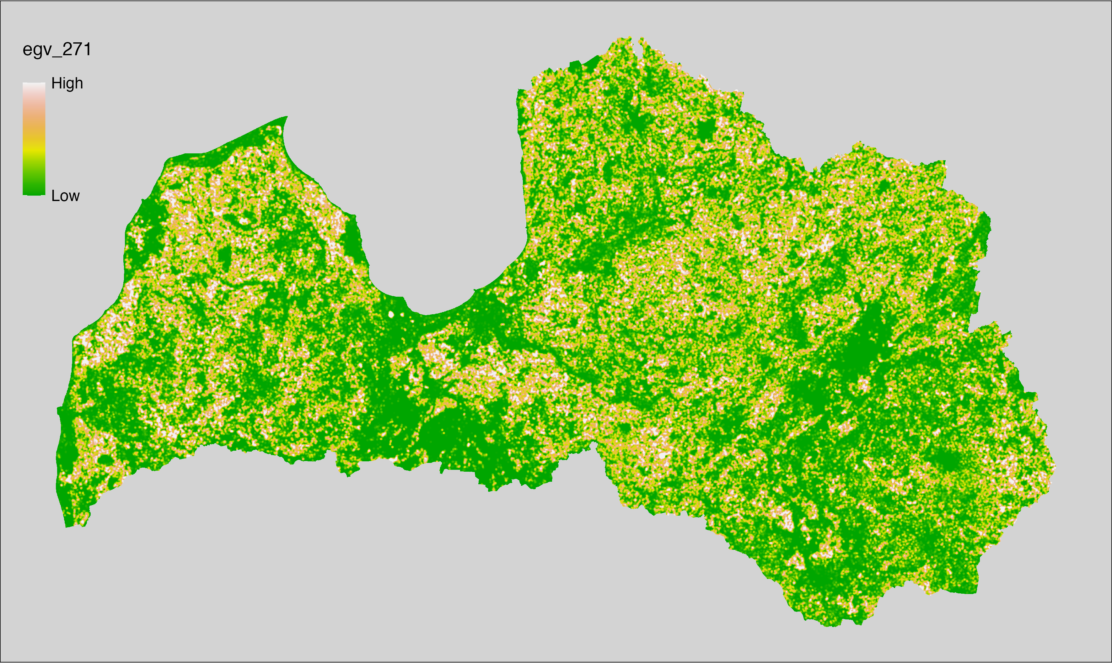
6.272 ForestsAge_ClearcutsLowStands_r1250
filename: ForestsAge_ClearcutsLowStands_r1250.tif
layername: egv_272
English name: Fractional cover of Clearcuts and Forest Stands lower than 5 m within the 1.25 km landscape
Latvian name: Izcirtumu un mežaudžu līdz 5 m augstumam platības īpatsvars 1,25 km ainavā
Procedure: The cover fraction within a radius of 1250 m around the analysis grid cell
is calculated as the area-weighted sum of the analysis cells inside
the buffer, using the workflow egvtools::radius_function(). During the calculation of the landscape
metric, inverse distance weighted (power = 2) gap filling on the output is
applied to ensure no missing values at the edges. Then the layer is
rewritten to set its name. Finally, the layer is standardised by
subtracting the arithmetic mean and dividing by the root mean squared error.
Code
# libs ----
if(!require(terra)) {install.packages("terra"); require(terra)}
if(!require(egvtools)) {remotes::install_github("aavotins/egvtools"); require(egvtools)}
# Templates -----
template100=rast("./Templates/TemplateRasters/LV100m_10km.tif")
# radii ----
radius_function(
kvadrati_path = "./Templates/TemplateGrids/tiles/",
radii_path = "./Templates/TemplateGridPoints/tiles/",
tikls100_path = "./Templates/TemplateGrids/tikls100_sauzeme.parquet",
template_path = "./Templates/TemplateRasters/LV100m_10km.tif",
input_layers = c("./RasterGrids_100m/2024/RAW/ForestsAge_ClearcutsLowStands_cell.tif"),
layer_prefixes = c("ForestsAge_ClearcutsLowStands"),
output_dir = "./RasterGrids_100m/2024/RAW/",
n_workers = 6,
radii = c("r1250"),
radius_mode = "sparse",
extract_fun = "mean",
fill_missing = TRUE,
IDW_weight = 2,
future_max_size = 40 * 1024^3)
# ForestsAge_ClearcutsLowStands_r1250.tif egv_272
slanis=rast("./RasterGrids_100m/2024/RAW/ForestsAge_ClearcutsLowStands_r1250.tif")
names(slanis)="egv_272"
slanis2=project(slanis,template100)
writeRaster(slanis2,
"./RasterGrids_100m/2024/RAW/ForestsAge_ClearcutsLowStands_r1250.tif",
overwrite=TRUE)
# standardisation ----
if(!require(terra)) {install.packages("terra"); require(terra)}
if(!require(tidyverse)) {install.packages("tidyverse"); require(tidyverse)}
nosaukums="ForestsAge_ClearcutsLowStands_r1250.tif"
ielasisanas_cels=paste0("./RasterGrids_100m/2024/RAW/",nosaukums)
saglabasanas_cels=paste0("./RasterGrids_100m/2024/Scaled/",nosaukums)
slanis=rast(ielasisanas_cels)
videjais=global(slanis,fun="mean",na.rm=TRUE)
centrets=slanis-videjais[,1]
standartnovirze=terra::global(centrets,fun="rms",na.rm=TRUE)
merogots=centrets/standartnovirze[,1]
writeRaster(merogots,
filename=saglabasanas_cels,
overwrite=TRUE)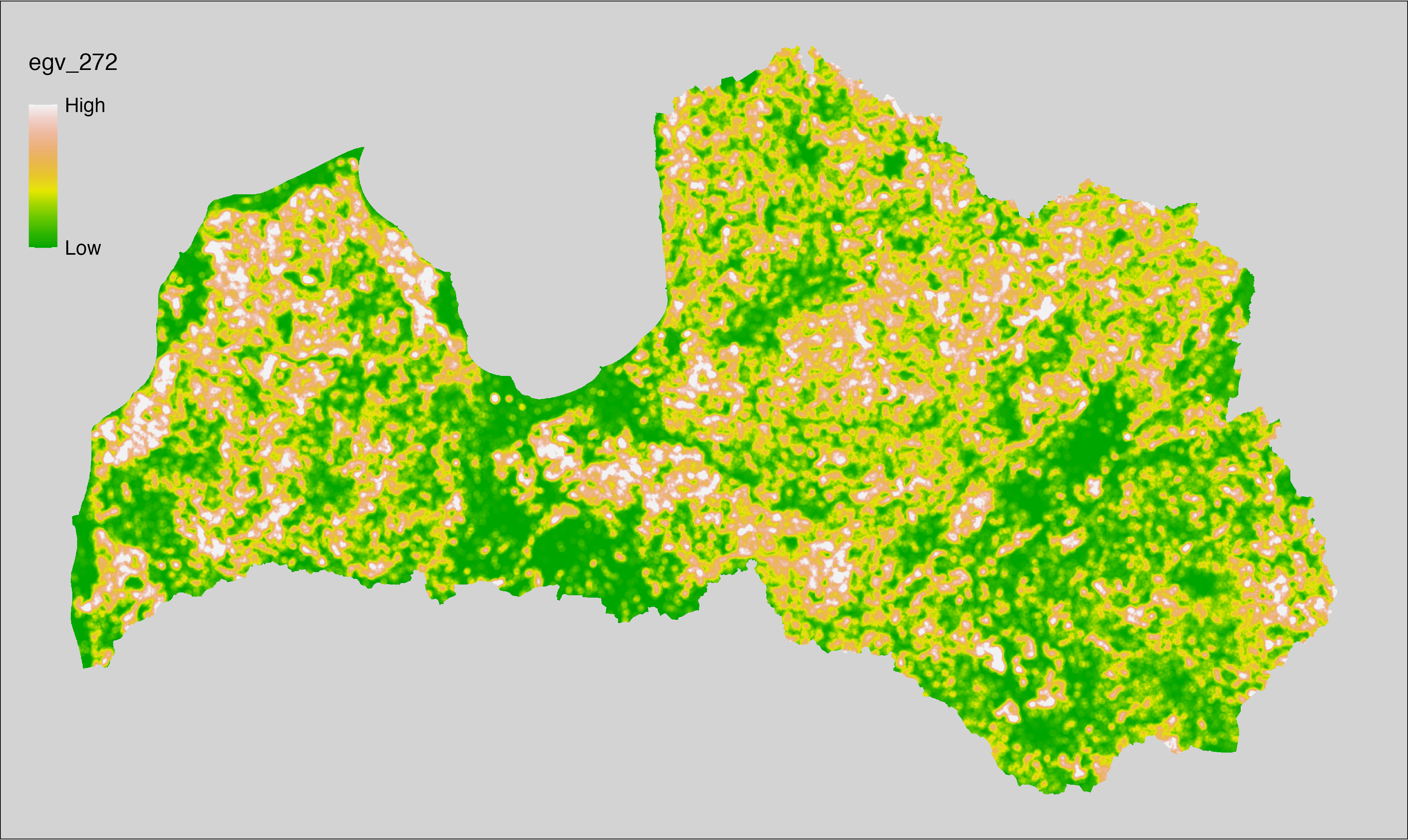
6.273 ForestsAge_ClearcutsLowStands_r3000
filename: ForestsAge_ClearcutsLowStands_r3000.tif
layername: egv_273
English name: Fractional cover of Clearcuts and Forest Stands lower than 5 m within the 3 km landscape
Latvian name: Izcirtumu un mežaudžu līdz 5 m augstumam platības īpatsvars 3 km ainavā
Procedure: The cover fraction within a radius of 3000 m around the analysis grid cell
is calculated as the area-weighted sum of the analysis cells inside
the buffer, using the workflow egvtools::radius_function(). During the calculation of the landscape
metric, inverse distance weighted (power = 2) gap filling on the output is
applied to ensure no missing values at the edges. Then the layer is
rewritten to set its name. Finally, the layer is standardised by
subtracting the arithmetic mean and dividing by the root mean squared error.
Code
# libs ----
if(!require(terra)) {install.packages("terra"); require(terra)}
if(!require(egvtools)) {remotes::install_github("aavotins/egvtools"); require(egvtools)}
# Templates -----
template100=rast("./Templates/TemplateRasters/LV100m_10km.tif")
# radii ----
radius_function(
kvadrati_path = "./Templates/TemplateGrids/tiles/",
radii_path = "./Templates/TemplateGridPoints/tiles/",
tikls100_path = "./Templates/TemplateGrids/tikls100_sauzeme.parquet",
template_path = "./Templates/TemplateRasters/LV100m_10km.tif",
input_layers = c("./RasterGrids_100m/2024/RAW/ForestsAge_ClearcutsLowStands_cell.tif"),
layer_prefixes = c("ForestsAge_ClearcutsLowStands"),
output_dir = "./RasterGrids_100m/2024/RAW/",
n_workers = 6,
radii = c("r3000"),
radius_mode = "sparse",
extract_fun = "mean",
fill_missing = TRUE,
IDW_weight = 2,
future_max_size = 40 * 1024^3)
# ForestsAge_ClearcutsLowStands_r3000.tif egv_273
slanis=rast("./RasterGrids_100m/2024/RAW/ForestsAge_ClearcutsLowStands_r3000.tif")
names(slanis)="egv_273"
slanis2=project(slanis,template100)
writeRaster(slanis2,
"./RasterGrids_100m/2024/RAW/ForestsAge_ClearcutsLowStands_r3000.tif",
overwrite=TRUE)
# standardisation ----
if(!require(terra)) {install.packages("terra"); require(terra)}
if(!require(tidyverse)) {install.packages("tidyverse"); require(tidyverse)}
nosaukums="ForestsAge_ClearcutsLowStands_r3000.tif"
ielasisanas_cels=paste0("./RasterGrids_100m/2024/RAW/",nosaukums)
saglabasanas_cels=paste0("./RasterGrids_100m/2024/Scaled/",nosaukums)
slanis=rast(ielasisanas_cels)
videjais=global(slanis,fun="mean",na.rm=TRUE)
centrets=slanis-videjais[,1]
standartnovirze=terra::global(centrets,fun="rms",na.rm=TRUE)
merogots=centrets/standartnovirze[,1]
writeRaster(merogots,
filename=saglabasanas_cels,
overwrite=TRUE)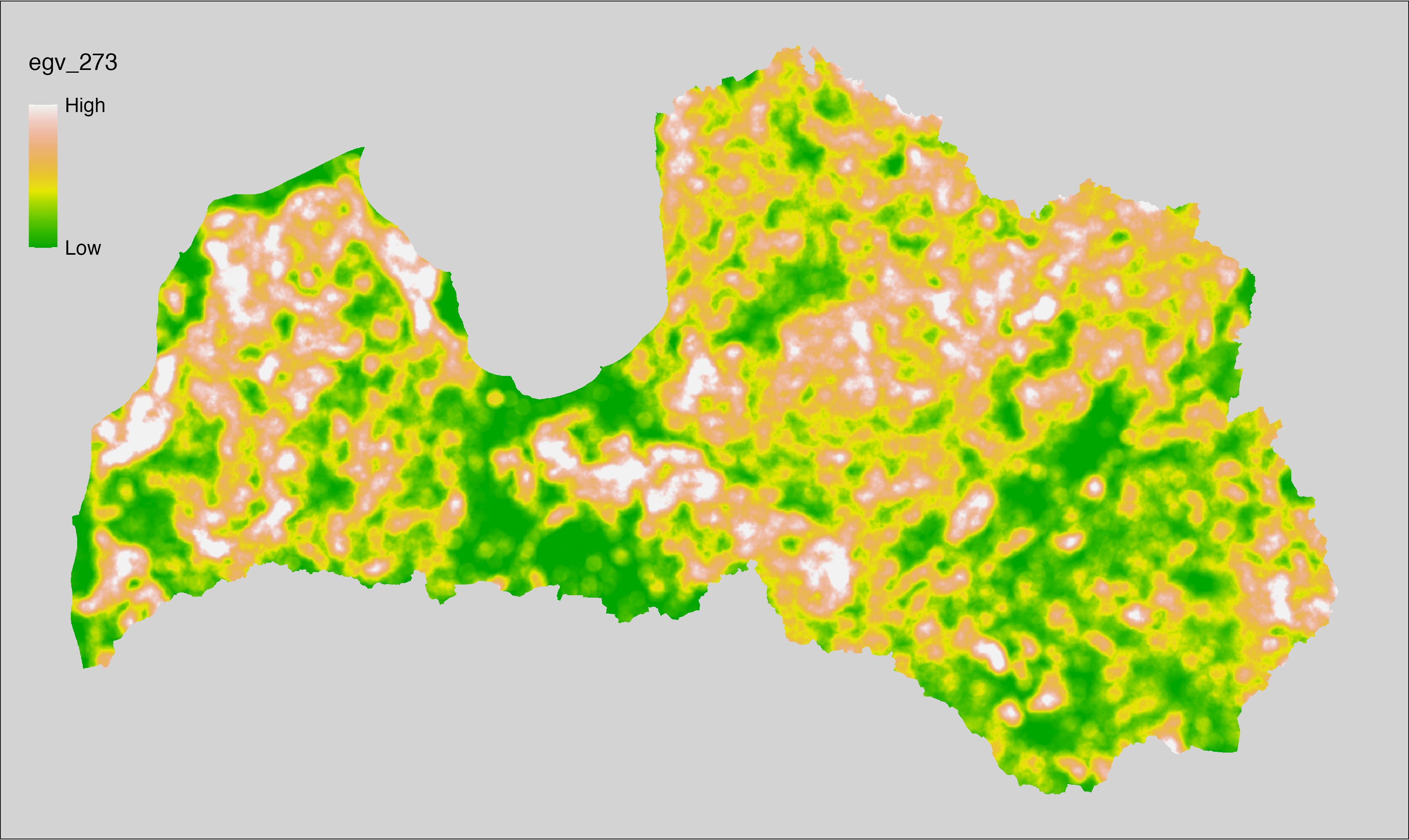
6.274 ForestsAge_ClearcutsLowStands_r10000
filename: ForestsAge_ClearcutsLowStands_r10000.tif
layername: egv_274
English name: Fractional cover of Clearcuts and Forest Stands lower than 5 m within the 10 km landscape
Latvian name: Izcirtumu un mežaudžu līdz 5 m augstumam platības īpatsvars 10 km ainavā
Procedure: The cover fraction within a radius of 10000 m around the analysis grid cell
is calculated as the area-weighted sum of the analysis cells inside
the buffer, using the workflow egvtools::radius_function(). During the calculation of the landscape
metric, inverse distance weighted (power = 2) gap filling on the output is
applied to ensure no missing values at the edges. Then the layer is
rewritten to set its name. Finally, the layer is standardised by
subtracting the arithmetic mean and dividing by the root mean squared error.
Code
# libs ----
if(!require(terra)) {install.packages("terra"); require(terra)}
if(!require(egvtools)) {remotes::install_github("aavotins/egvtools"); require(egvtools)}
# Templates -----
template100=rast("./Templates/TemplateRasters/LV100m_10km.tif")
# radii ----
radius_function(
kvadrati_path = "./Templates/TemplateGrids/tiles/",
radii_path = "./Templates/TemplateGridPoints/tiles/",
tikls100_path = "./Templates/TemplateGrids/tikls100_sauzeme.parquet",
template_path = "./Templates/TemplateRasters/LV100m_10km.tif",
input_layers = c("./RasterGrids_100m/2024/RAW/ForestsAge_ClearcutsLowStands_cell.tif"),
layer_prefixes = c("ForestsAge_ClearcutsLowStands"),
output_dir = "./RasterGrids_100m/2024/RAW/",
n_workers = 6,
radii = c("r10000"),
radius_mode = "sparse",
extract_fun = "mean",
fill_missing = TRUE,
IDW_weight = 2,
future_max_size = 40 * 1024^3)
# ForestsAge_ClearcutsLowStands_r10000.tif egv_274
slanis=rast("./RasterGrids_100m/2024/RAW/ForestsAge_ClearcutsLowStands_r10000.tif")
names(slanis)="egv_274"
slanis2=project(slanis,template100)
writeRaster(slanis2,
"./RasterGrids_100m/2024/RAW/ForestsAge_ClearcutsLowStands_r10000.tif",
overwrite=TRUE)
# standardisation ----
if(!require(terra)) {install.packages("terra"); require(terra)}
if(!require(tidyverse)) {install.packages("tidyverse"); require(tidyverse)}
nosaukums="ForestsAge_ClearcutsLowStands_r10000.tif"
ielasisanas_cels=paste0("./RasterGrids_100m/2024/RAW/",nosaukums)
saglabasanas_cels=paste0("./RasterGrids_100m/2024/Scaled/",nosaukums)
slanis=rast(ielasisanas_cels)
videjais=global(slanis,fun="mean",na.rm=TRUE)
centrets=slanis-videjais[,1]
standartnovirze=terra::global(centrets,fun="rms",na.rm=TRUE)
merogots=centrets/standartnovirze[,1]
writeRaster(merogots,
filename=saglabasanas_cels,
overwrite=TRUE)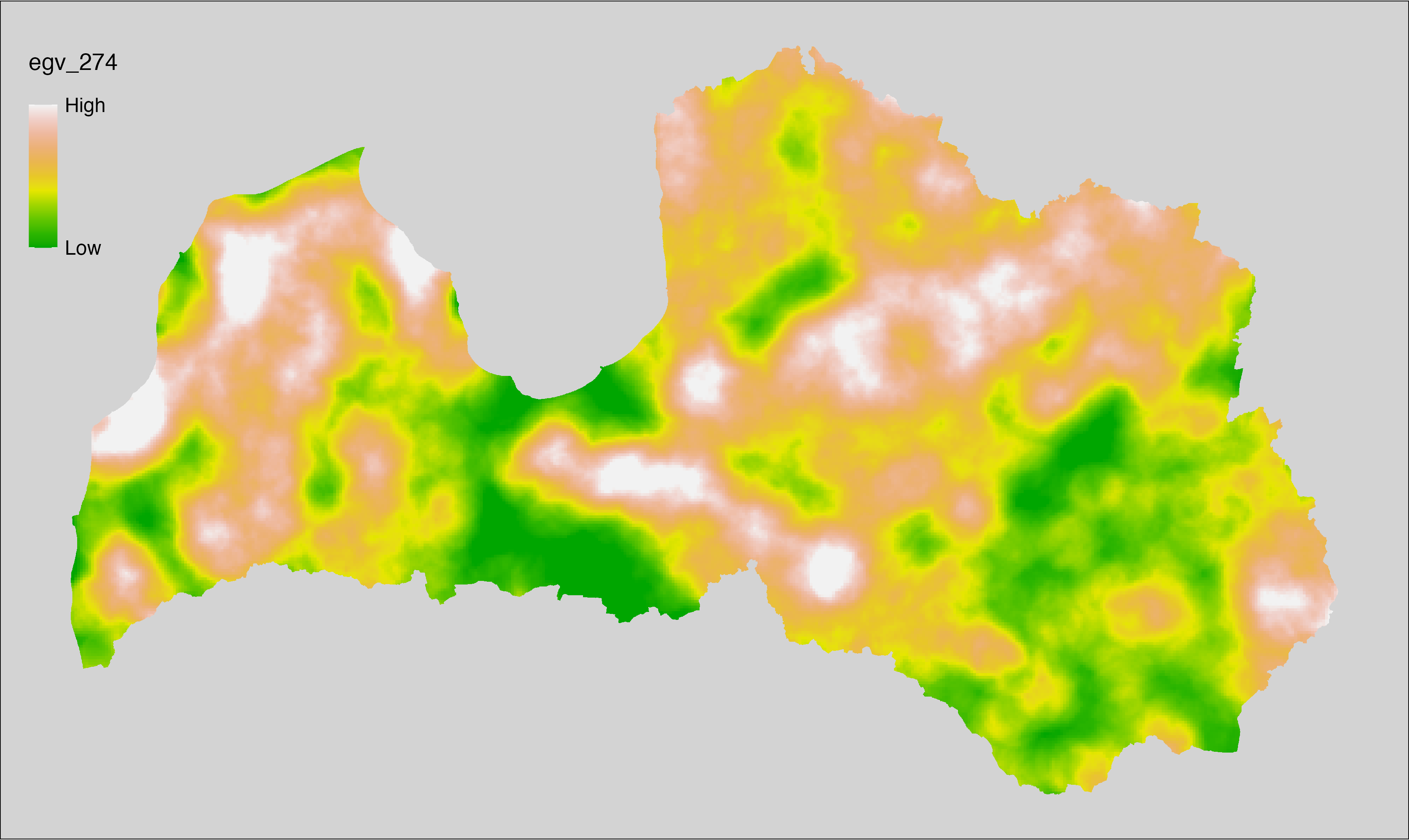
6.275 ForestsAge_Middle_cell
filename: ForestsAge_Middle_cell.tif
layername: egv_275
English name: Fractional cover of Middle-Aged Forest Stands within the analysis cell (1 ha)
Latvian name: Vidēja vecuma un briestaudžu platības īpatsvars analīzes šūnā (1 ha)
Procedure: Most EGVs describing forests are spatially restricted to areas outside of clearcuts and dead stands. This mask is created using a combination of the State Forest Service’s State Forest Registry land category 12 and 14, and The Global Forest Watch pixels classified as lost tree canopy cover since 2020 (raster layer matching input, presence = 1, absence = 0).
To prepare this
EGV, stands in land category 10 and age groups two and three are selected from
State Forest Service’s State Forest Registry and rasterised.
Rasterisation is performed using the workflow egvtools::polygon2input() (presence = 1,
absence = 0), restricting presence locations only outside the clearcut mask. The resulting layer
is then aggregated to EGV resolution using the workflow egvtools::input2egv(), which
calculates the arithmetic mean to determine the cover fraction. During
aggregation, inverse distance weighted (power = 2) gap filling on the output is
applied to ensure no missing values at the edges. Finally, the layer is
standardised by subtracting the arithmetic mean and dividing by the root mean squared
error.
Code
# libs ----
if(!require(egvtools)) {remotes::install_github("aavotins/egvtools"); require(egvtools)}
if(!require(terra)) {install.packages("terra"); require(terra)}
if(!require(sf)) {install.packages("sf"); require(sf)}
if(!require(tidyverse)) {install.packages("tidyverse"); require(tidyverse)}
if(!require(sfarrow)) {install.packages("sfarrow"); require(sfarrow)}
if(!require(readxl)) {install.packages("readxl"); require(readxl)}
if(!require(raster)) {install.packages("raster"); require(raster)}
if(!require(fasterize)) {install.packages("fasterize"); require(fasterize)}
# templates ----
template100=rast("./Templates/TemplateRasters/LV100m_10km.tif")
template10=rast("./Templates/TemplateRasters/LV10m_10km.tif")
rastrs10=raster(template10)
nulls10=rast("./Templates/TemplateRasters/nulls_LV10m_10km.tif")
nulls100=rast("./Templates/TemplateRasters/nulls_LV100m_10km.tif")
# simple landscape ----
simple_landscape=rast("RasterGrids_10m/2024/Ainava_vienk_mask.tif")
# mvr ----
mvr=st_read_parquet("./Geodata/2024/MVR/nogabali_2024janv.parquet")
mvr$yes=1
# clear cut mask ----
izcirtumi=mvr %>%
filter(zkat %in% c("12","14")) %>%
dplyr::select(yes)
r_izcirtumi_mvr=fasterize(izcirtumi,rastrs10,field="yes")
t_izcirtumi_mvr=rast(r_izcirtumi_mvr)
plot(t_izcirtumi_mvr)
tcl=rast("./Geodata/2024/Trees/GFW/TreeCoverLoss_v1_12.tif")
tcl2=ifel(tcl<20,0,1)
tclX=cover(tcl2,nulls10)
plot(tclX)
clearcut_mask=cover(t_izcirtumi_mvr,tclX,
filename="./RasterGrids_10m/2024/Mask_clearcuts.tif",
overwrite=TRUE)
plot(clearcut_mask)
rm(izcirtumi)
rm(r_izcirtumi_mvr)
rm(t_izcirtumi_mvr)
rm(tcl)
rm(tcl2)
rm(tclX)
# ForestsAge_Middle_cell.tif egv_275 ----
videjas_audzes=mvr %>%
filter(zkat=="10") %>%
#filter(h10>=5) %>%
filter(vgr %in% c("2","3")) %>%
dplyr::select(yes)
p2i_rez=egvtools::polygon2input(vector_data = videjas_audzes,
template_path = "./Templates/TemplateRasters/LV10m_10km.tif",
out_path = "./RasterGrids_10m/2024/",
file_name = "ForestsAge_Middle_input.tif",
value_field = "yes",
restrict_to = clearcut_mask,
restrict_values = 0,
prepare=FALSE,
background_raster = "./Templates/TemplateRasters/nulls_LV10m_10km.tif",
plot_result = TRUE)
p2i_rez
i2e_rez=egvtools::input2egv(input=paste0("./RasterGrids_10m/2024/",
"ForestsAge_Middle_input.tif"),
egv_template= "./Templates/TemplateRasters/LV100m_10km.tif",
summary_function = "average",
missing_job = "FillOutput",
outlocation = "./RasterGrids_100m/2024/RAW/",
outfilename = "ForestsAge_Middle_cell.tif",
layername = "egv_275",
idw_weight = 2,
plot_gaps = FALSE,plot_final = TRUE)
i2e_rez
rm(videjas_audzes)
rm(p2i_rez)
rm(i2e_rez)
unlink("./RasterGrids_10m/2024/ForestsAge_Middle_input.tif")
# standardisation ----
if(!require(terra)) {install.packages("terra"); require(terra)}
if(!require(tidyverse)) {install.packages("tidyverse"); require(tidyverse)}
nosaukums="ForestsAge_Middle_cell.tif"
ielasisanas_cels=paste0("./RasterGrids_100m/2024/RAW/",nosaukums)
saglabasanas_cels=paste0("./RasterGrids_100m/2024/Scaled/",nosaukums)
slanis=rast(ielasisanas_cels)
videjais=global(slanis,fun="mean",na.rm=TRUE)
centrets=slanis-videjais[,1]
standartnovirze=terra::global(centrets,fun="rms",na.rm=TRUE)
merogots=centrets/standartnovirze[,1]
writeRaster(merogots,
filename=saglabasanas_cels,
overwrite=TRUE)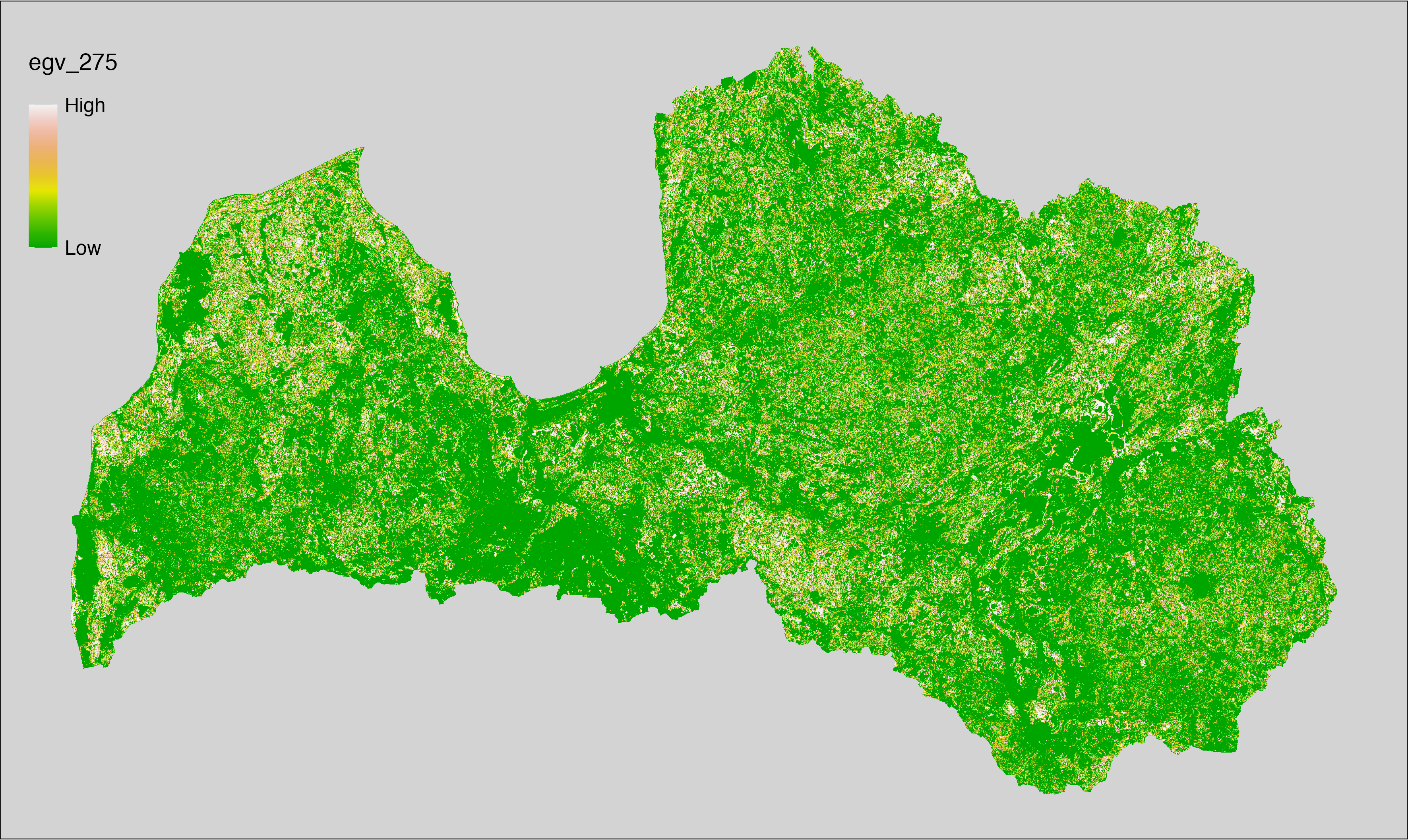
6.276 ForestsAge_Middle_r500
filename: ForestsAge_Middle_r500.tif
layername: egv_276
English name: Fractional cover of Middle-Aged Forest Stands within the 0.5 km landscape
Latvian name: Vidēja vecuma un briestaudžu platības īpatsvars 0,5 km ainavā
Procedure: The cover fraction within a radius of 500 m around the analysis grid cell is
calculated as the area-weighted sum of the analysis cells inside the
buffer, using the workflow egvtools::radius_function(). During the calculation of the landscape metric,
inverse distance weighted (power = 2) gap filling on the output is applied
to ensure no missing values at the edges. Then the layer is rewritten to set
its name. Finally, the layer is standardised by subtracting the arithmetic
mean and dividing by the root mean squared error.
Code
# libs ----
if(!require(terra)) {install.packages("terra"); require(terra)}
if(!require(egvtools)) {remotes::install_github("aavotins/egvtools"); require(egvtools)}
# Templates -----
template100=rast("./Templates/TemplateRasters/LV100m_10km.tif")
# radii ----
radius_function(
kvadrati_path = "./Templates/TemplateGrids/tiles/",
radii_path = "./Templates/TemplateGridPoints/tiles/",
tikls100_path = "./Templates/TemplateGrids/tikls100_sauzeme.parquet",
template_path = "./Templates/TemplateRasters/LV100m_10km.tif",
input_layers = c("./RasterGrids_100m/2024/RAW/ForestsAge_Middle_cell.tif"),
layer_prefixes = c("ForestsAge_Middle"),
output_dir = "./RasterGrids_100m/2024/RAW/",
n_workers = 6,
radii = c("r500"),
radius_mode = "sparse",
extract_fun = "mean",
fill_missing = TRUE,
IDW_weight = 2,
future_max_size = 40 * 1024^3)
# ForestsAge_Middle_r500.tif egv_276
slanis=rast("./RasterGrids_100m/2024/RAW/ForestsAge_Middle_r500.tif")
names(slanis)="egv_276"
slanis2=project(slanis,template100)
writeRaster(slanis2,
"./RasterGrids_100m/2024/RAW/ForestsAge_Middle_r500.tif",
overwrite=TRUE)
# standardisation ----
if(!require(terra)) {install.packages("terra"); require(terra)}
if(!require(tidyverse)) {install.packages("tidyverse"); require(tidyverse)}
nosaukums="ForestsAge_Middle_r500.tif"
ielasisanas_cels=paste0("./RasterGrids_100m/2024/RAW/",nosaukums)
saglabasanas_cels=paste0("./RasterGrids_100m/2024/Scaled/",nosaukums)
slanis=rast(ielasisanas_cels)
videjais=global(slanis,fun="mean",na.rm=TRUE)
centrets=slanis-videjais[,1]
standartnovirze=terra::global(centrets,fun="rms",na.rm=TRUE)
merogots=centrets/standartnovirze[,1]
writeRaster(merogots,
filename=saglabasanas_cels,
overwrite=TRUE)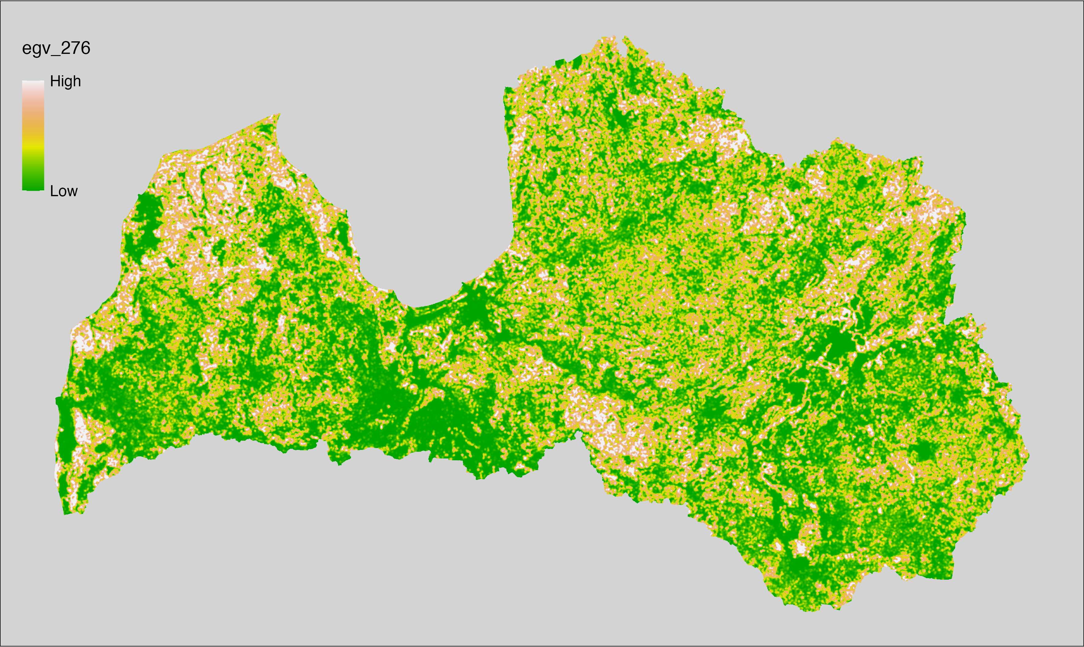
6.277 ForestsAge_Middle_r1250
filename: ForestsAge_Middle_r1250.tif
layername: egv_277
English name: Fractional cover of Middle-Aged Forest Stands within the 1.25 km landscape
Latvian name: Vidēja vecuma un briestaudžu platības īpatsvars 1,25 km ainavā
Procedure: The cover fraction within a radius of 1250 m around the analysis grid cell
is calculated as the area-weighted sum of the analysis cells inside
the buffer, using the workflow egvtools::radius_function(). During the calculation of the landscape
metric, inverse distance weighted (power = 2) gap filling on the output is
applied to ensure no missing values at the edges. Then the layer is
rewritten to set its name. Finally, the layer is standardised by
subtracting the arithmetic mean and dividing by the root mean squared error.
Code
# libs ----
if(!require(terra)) {install.packages("terra"); require(terra)}
if(!require(egvtools)) {remotes::install_github("aavotins/egvtools"); require(egvtools)}
# Templates -----
template100=rast("./Templates/TemplateRasters/LV100m_10km.tif")
# radii ----
radius_function(
kvadrati_path = "./Templates/TemplateGrids/tiles/",
radii_path = "./Templates/TemplateGridPoints/tiles/",
tikls100_path = "./Templates/TemplateGrids/tikls100_sauzeme.parquet",
template_path = "./Templates/TemplateRasters/LV100m_10km.tif",
input_layers = c("./RasterGrids_100m/2024/RAW/ForestsAge_Middle_cell.tif"),
layer_prefixes = c("ForestsAge_Middle"),
output_dir = "./RasterGrids_100m/2024/RAW/",
n_workers = 6,
radii = c("r1250"),
radius_mode = "sparse",
extract_fun = "mean",
fill_missing = TRUE,
IDW_weight = 2,
future_max_size = 40 * 1024^3)
# ForestsAge_Middle_r1250.tif egv_277
slanis=rast("./RasterGrids_100m/2024/RAW/ForestsAge_Middle_r1250.tif")
names(slanis)="egv_277"
slanis2=project(slanis,template100)
writeRaster(slanis2,
"./RasterGrids_100m/2024/RAW/ForestsAge_Middle_r1250.tif",
overwrite=TRUE)
# standardisation ----
if(!require(terra)) {install.packages("terra"); require(terra)}
if(!require(tidyverse)) {install.packages("tidyverse"); require(tidyverse)}
nosaukums="ForestsAge_Middle_r1250.tif"
ielasisanas_cels=paste0("./RasterGrids_100m/2024/RAW/",nosaukums)
saglabasanas_cels=paste0("./RasterGrids_100m/2024/Scaled/",nosaukums)
slanis=rast(ielasisanas_cels)
videjais=global(slanis,fun="mean",na.rm=TRUE)
centrets=slanis-videjais[,1]
standartnovirze=terra::global(centrets,fun="rms",na.rm=TRUE)
merogots=centrets/standartnovirze[,1]
writeRaster(merogots,
filename=saglabasanas_cels,
overwrite=TRUE)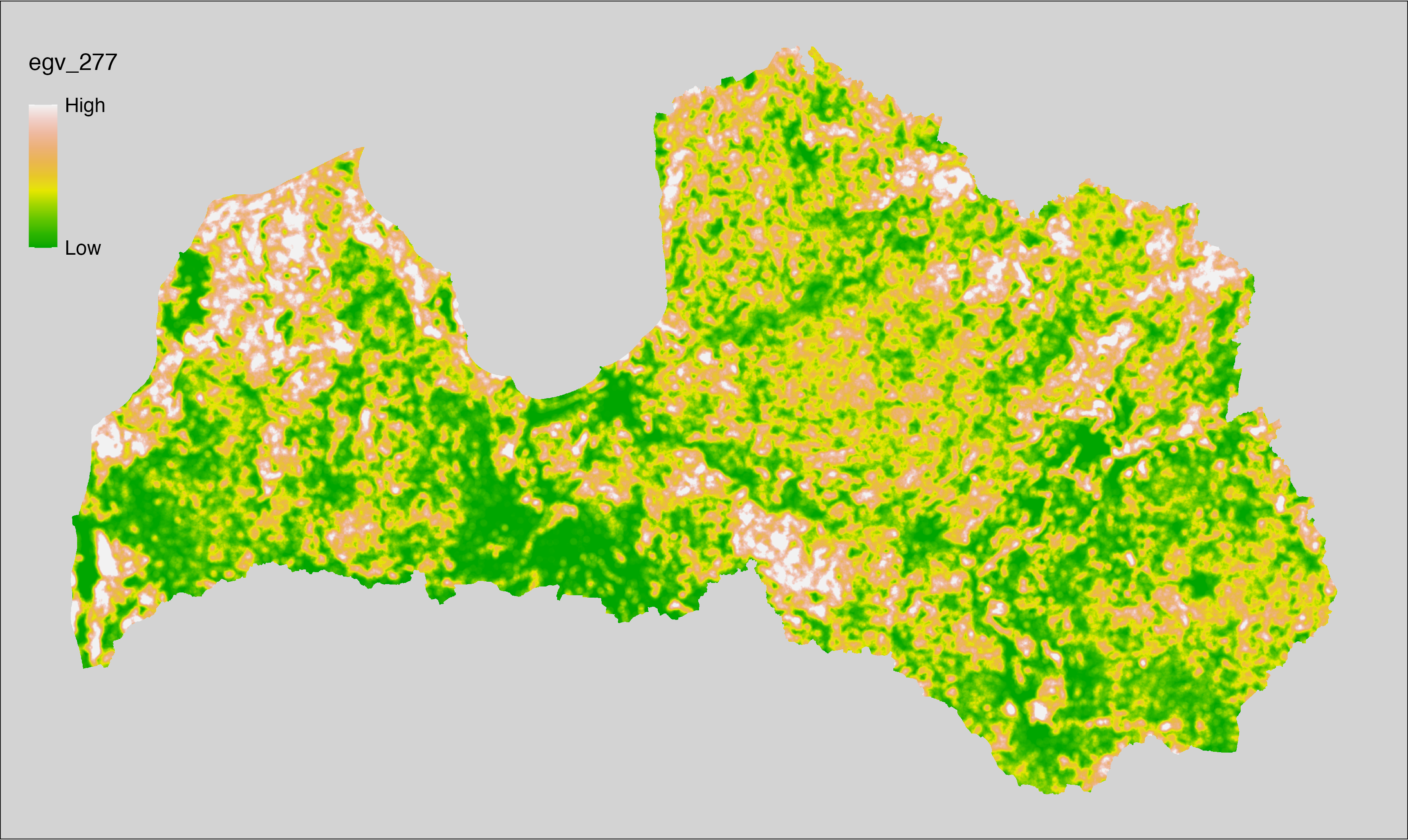
6.278 ForestsAge_Middle_r3000
filename: ForestsAge_Middle_r3000.tif
layername: egv_278
English name: Fractional cover of Middle-Aged Forest Stands within the 3 km landscape
Latvian name: Vidēja vecuma un briestaudžu platības īpatsvars 3 km ainavā
Procedure: The cover fraction within a radius of 3000 m around the analysis grid cell
is calculated as the area-weighted sum of the analysis cells inside
the buffer, using the workflow egvtools::radius_function(). During the calculation of the landscape
metric, inverse distance weighted (power = 2) gap filling on the output is
applied to ensure no missing values at the edges. Then the layer is
rewritten to set its name. Finally, the layer is standardised by
subtracting the arithmetic mean and dividing by the root mean squared error.
Code
# libs ----
if(!require(terra)) {install.packages("terra"); require(terra)}
if(!require(egvtools)) {remotes::install_github("aavotins/egvtools"); require(egvtools)}
# Templates -----
template100=rast("./Templates/TemplateRasters/LV100m_10km.tif")
# radii ----
radius_function(
kvadrati_path = "./Templates/TemplateGrids/tiles/",
radii_path = "./Templates/TemplateGridPoints/tiles/",
tikls100_path = "./Templates/TemplateGrids/tikls100_sauzeme.parquet",
template_path = "./Templates/TemplateRasters/LV100m_10km.tif",
input_layers = c("./RasterGrids_100m/2024/RAW/ForestsAge_Middle_cell.tif"),
layer_prefixes = c("ForestsAge_Middle"),
output_dir = "./RasterGrids_100m/2024/RAW/",
n_workers = 6,
radii = c("r3000"),
radius_mode = "sparse",
extract_fun = "mean",
fill_missing = TRUE,
IDW_weight = 2,
future_max_size = 40 * 1024^3)
# ForestsAge_Middle_r3000.tif egv_278
slanis=rast("./RasterGrids_100m/2024/RAW/ForestsAge_Middle_r3000.tif")
names(slanis)="egv_278"
slanis2=project(slanis,template100)
writeRaster(slanis2,
"./RasterGrids_100m/2024/RAW/ForestsAge_Middle_r3000.tif",
overwrite=TRUE)
# standardisation ----
if(!require(terra)) {install.packages("terra"); require(terra)}
if(!require(tidyverse)) {install.packages("tidyverse"); require(tidyverse)}
nosaukums="ForestsAge_Middle_r3000.tif"
ielasisanas_cels=paste0("./RasterGrids_100m/2024/RAW/",nosaukums)
saglabasanas_cels=paste0("./RasterGrids_100m/2024/Scaled/",nosaukums)
slanis=rast(ielasisanas_cels)
videjais=global(slanis,fun="mean",na.rm=TRUE)
centrets=slanis-videjais[,1]
standartnovirze=terra::global(centrets,fun="rms",na.rm=TRUE)
merogots=centrets/standartnovirze[,1]
writeRaster(merogots,
filename=saglabasanas_cels,
overwrite=TRUE)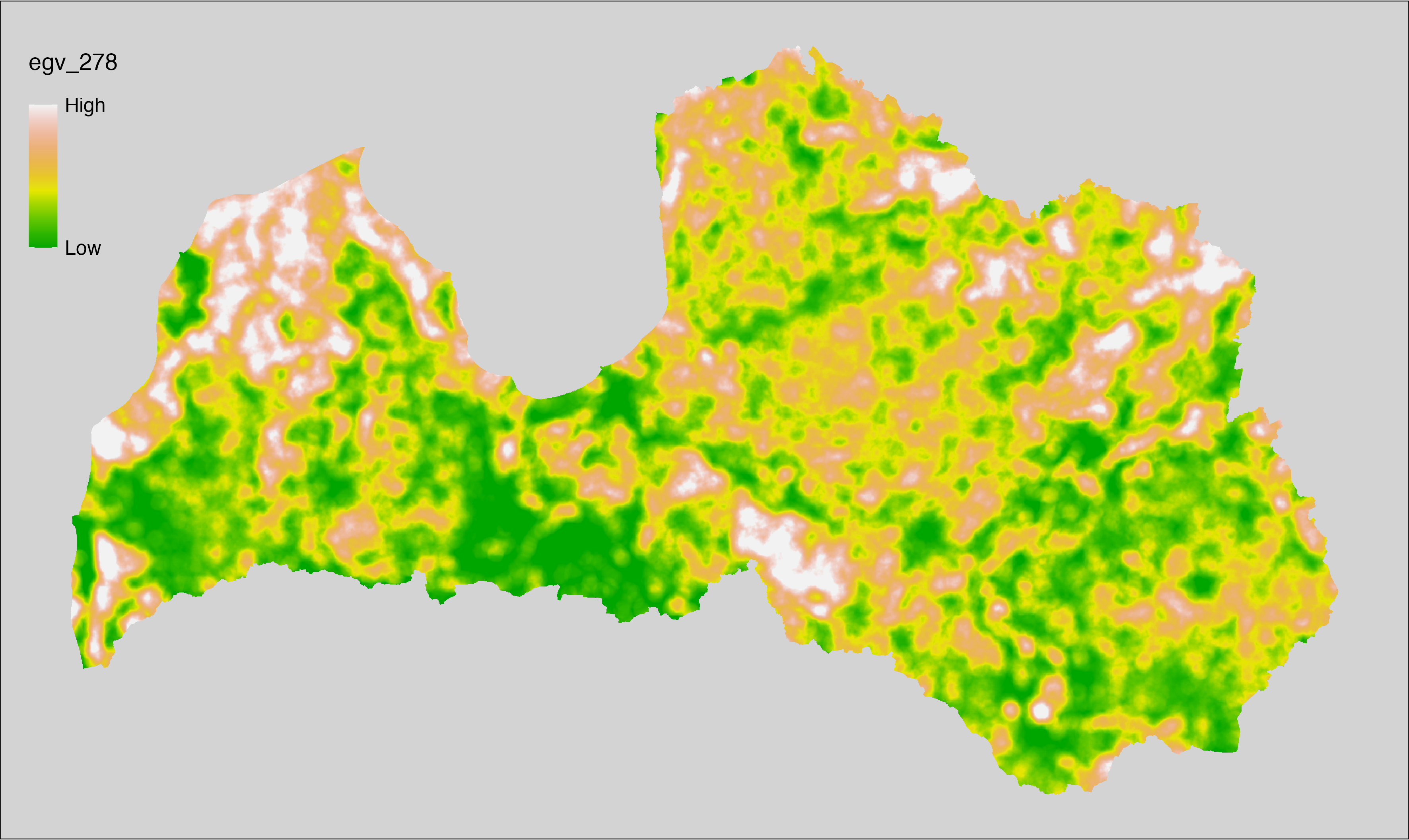
6.279 ForestsAge_Middle_r10000
filename: ForestsAge_Middle_r10000.tif
layername: egv_279
English name: Fractional cover of Middle-Aged Forest Stands within the 10 km landscape
Latvian name: Vidēja vecuma un briestaudžu platības īpatsvars 10 km ainavā
Procedure: The cover fraction within a radius of 10000 m around the analysis grid cell
is calculated as the area-weighted sum of the analysis cells inside
the buffer, using the workflow egvtools::radius_function(). During the calculation of the landscape
metric, inverse distance weighted (power = 2) gap filling on the output is
applied to ensure no missing values at the edges. Then the layer is
rewritten to set its name. Finally, the layer is standardised by
subtracting the arithmetic mean and dividing by the root mean squared error.
Code
# libs ----
if(!require(terra)) {install.packages("terra"); require(terra)}
if(!require(egvtools)) {remotes::install_github("aavotins/egvtools"); require(egvtools)}
# Templates -----
template100=rast("./Templates/TemplateRasters/LV100m_10km.tif")
# radii ----
radius_function(
kvadrati_path = "./Templates/TemplateGrids/tiles/",
radii_path = "./Templates/TemplateGridPoints/tiles/",
tikls100_path = "./Templates/TemplateGrids/tikls100_sauzeme.parquet",
template_path = "./Templates/TemplateRasters/LV100m_10km.tif",
input_layers = c("./RasterGrids_100m/2024/RAW/ForestsAge_Middle_cell.tif"),
layer_prefixes = c("ForestsAge_Middle"),
output_dir = "./RasterGrids_100m/2024/RAW/",
n_workers = 6,
radii = c("r10000"),
radius_mode = "sparse",
extract_fun = "mean",
fill_missing = TRUE,
IDW_weight = 2,
future_max_size = 40 * 1024^3)
# ForestsAge_Middle_r10000.tif egv_279
slanis=rast("./RasterGrids_100m/2024/RAW/ForestsAge_Middle_r10000.tif")
names(slanis)="egv_279"
slanis2=project(slanis,template100)
writeRaster(slanis2,
"./RasterGrids_100m/2024/RAW/ForestsAge_Middle_r10000.tif",
overwrite=TRUE)
# standardisation ----
if(!require(terra)) {install.packages("terra"); require(terra)}
if(!require(tidyverse)) {install.packages("tidyverse"); require(tidyverse)}
nosaukums="ForestsAge_Middle_r10000.tif"
ielasisanas_cels=paste0("./RasterGrids_100m/2024/RAW/",nosaukums)
saglabasanas_cels=paste0("./RasterGrids_100m/2024/Scaled/",nosaukums)
slanis=rast(ielasisanas_cels)
videjais=global(slanis,fun="mean",na.rm=TRUE)
centrets=slanis-videjais[,1]
standartnovirze=terra::global(centrets,fun="rms",na.rm=TRUE)
merogots=centrets/standartnovirze[,1]
writeRaster(merogots,
filename=saglabasanas_cels,
overwrite=TRUE)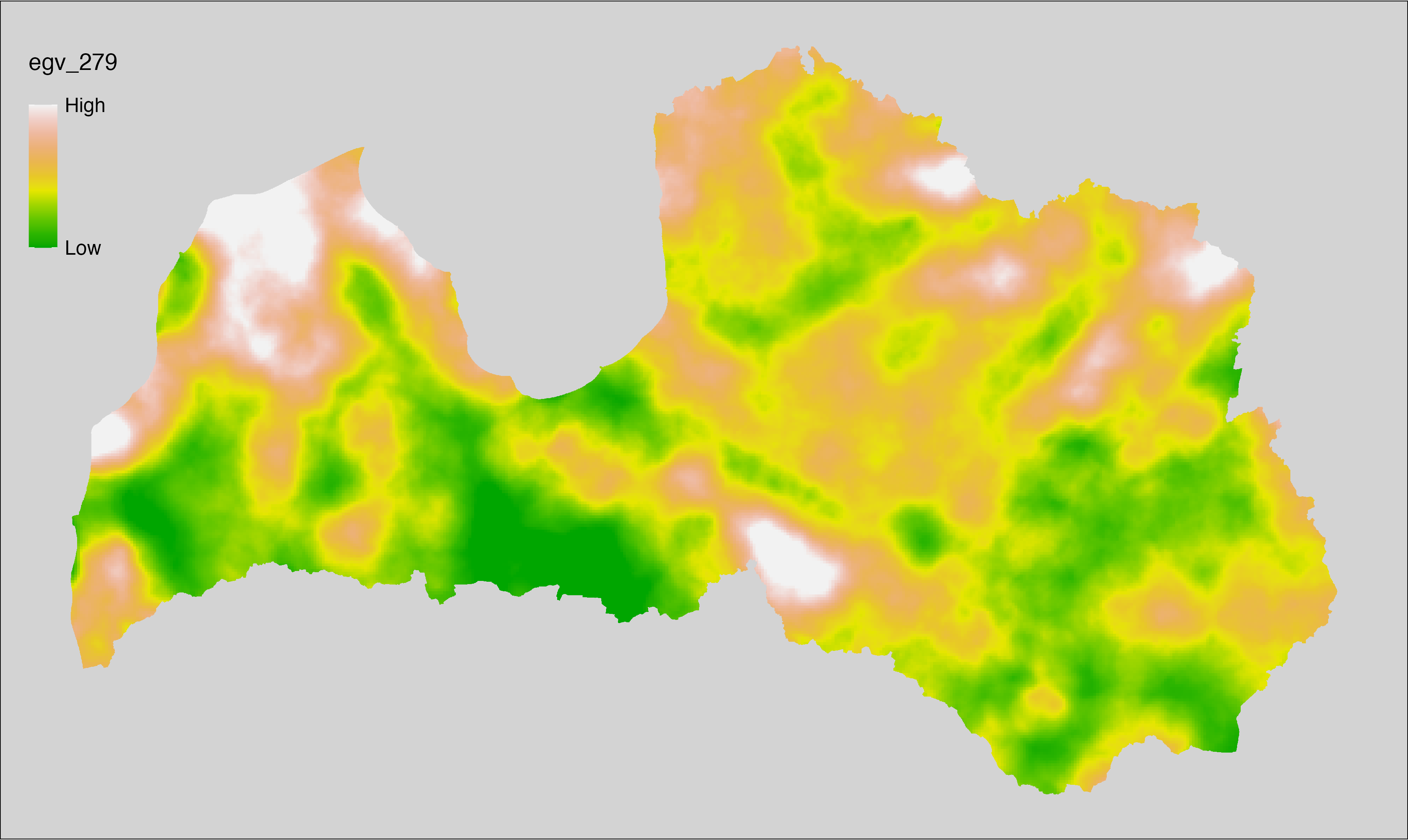
6.280 ForestsAge_Old_cell
filename: ForestsAge_Old_cell.tif
layername: egv_280
English name: Fractional cover of Old (over rotation age) Forest Stands within the analysis cell (1 ha)
Latvian name: Vecu (kopš cirtmeta) mežaudžu platības īpatsvars analīzes šūnā (1 ha)
Procedure: Most EGVs describing forests are spatially restricted to areas outside of clearcuts and dead stands. This mask is created using a combination of the State Forest Service’s State Forest Registry land category 12 and 14, and The Global Forest Watch pixels classified as lost tree canopy cover since 2020 (raster layer matching input, presence = 1, absence = 0).
To prepare this
EGV, stands in land category 10 and age groups four and five are selected from
State Forest Service’s State Forest Registry and rasterised.
Rasterisation is performed using the workflow egvtools::polygon2input() (presence = 1,
absence = 0), restricting presence locations only outside the clearcut mask. The resulting layer
is then aggregated to EGV resolution using the workflow egvtools::input2egv(), which
calculates the arithmetic mean to determine the cover fraction. During
aggregation, inverse distance weighted (power = 2) gap filling on the output is
applied to ensure no missing values at the edges. Finally, the layer is
standardised by subtracting the arithmetic mean and dividing by the root mean squared
error.
Code
# libs ----
if(!require(egvtools)) {remotes::install_github("aavotins/egvtools"); require(egvtools)}
if(!require(terra)) {install.packages("terra"); require(terra)}
if(!require(sf)) {install.packages("sf"); require(sf)}
if(!require(tidyverse)) {install.packages("tidyverse"); require(tidyverse)}
if(!require(sfarrow)) {install.packages("sfarrow"); require(sfarrow)}
if(!require(readxl)) {install.packages("readxl"); require(readxl)}
if(!require(raster)) {install.packages("raster"); require(raster)}
if(!require(fasterize)) {install.packages("fasterize"); require(fasterize)}
# templates ----
template100=rast("./Templates/TemplateRasters/LV100m_10km.tif")
template10=rast("./Templates/TemplateRasters/LV10m_10km.tif")
rastrs10=raster(template10)
nulls10=rast("./Templates/TemplateRasters/nulls_LV10m_10km.tif")
nulls100=rast("./Templates/TemplateRasters/nulls_LV100m_10km.tif")
# simple landscape ----
simple_landscape=rast("RasterGrids_10m/2024/Ainava_vienk_mask.tif")
# mvr ----
mvr=st_read_parquet("./Geodata/2024/MVR/nogabali_2024janv.parquet")
mvr$yes=1
# clear cut mask ----
izcirtumi=mvr %>%
filter(zkat %in% c("12","14")) %>%
dplyr::select(yes)
r_izcirtumi_mvr=fasterize(izcirtumi,rastrs10,field="yes")
t_izcirtumi_mvr=rast(r_izcirtumi_mvr)
plot(t_izcirtumi_mvr)
tcl=rast("./Geodata/2024/Trees/GFW/TreeCoverLoss_v1_12.tif")
tcl2=ifel(tcl<20,0,1)
tclX=cover(tcl2,nulls10)
plot(tclX)
clearcut_mask=cover(t_izcirtumi_mvr,tclX,
filename="./RasterGrids_10m/2024/Mask_clearcuts.tif",
overwrite=TRUE)
plot(clearcut_mask)
rm(izcirtumi)
rm(r_izcirtumi_mvr)
rm(t_izcirtumi_mvr)
rm(tcl)
rm(tcl2)
rm(tclX)
# ForestsAge_Old_cell.tif egv_280 ----
vecas=mvr %>%
filter(zkat=="10") %>%
#filter(h10>=5) %>%
filter(vgr %in% c("4","5")) %>%
dplyr::select(yes)
p2i_rez=egvtools::polygon2input(vector_data = vecas,
template_path = "./Templates/TemplateRasters/LV10m_10km.tif",
out_path = "./RasterGrids_10m/2024/",
file_name = "ForestsAge_Old_input.tif",
value_field = "yes",
restrict_to = clearcut_mask,
restrict_values = 0,
prepare=FALSE,
background_raster = "./Templates/TemplateRasters/nulls_LV10m_10km.tif",
plot_result = TRUE)
p2i_rez
i2e_rez=egvtools::input2egv(input=paste0("./RasterGrids_10m/2024/",
"ForestsAge_Old_input.tif"),
egv_template= "./Templates/TemplateRasters/LV100m_10km.tif",
summary_function = "average",
missing_job = "FillOutput",
outlocation = "./RasterGrids_100m/2024/RAW/",
outfilename = "ForestsAge_Old_cell.tif",
layername = "egv_280",
idw_weight = 2,
plot_gaps = FALSE,plot_final = TRUE)
i2e_rez
rm(vecas)
rm(p2i_rez)
rm(i2e_rez)
unlink("./RasterGrids_10m/2024/ForestsAge_Old_input.tif")
# standardisation ----
if(!require(terra)) {install.packages("terra"); require(terra)}
if(!require(tidyverse)) {install.packages("tidyverse"); require(tidyverse)}
nosaukums="ForestsAge_Old_cell.tif"
ielasisanas_cels=paste0("./RasterGrids_100m/2024/RAW/",nosaukums)
saglabasanas_cels=paste0("./RasterGrids_100m/2024/Scaled/",nosaukums)
slanis=rast(ielasisanas_cels)
videjais=global(slanis,fun="mean",na.rm=TRUE)
centrets=slanis-videjais[,1]
standartnovirze=terra::global(centrets,fun="rms",na.rm=TRUE)
merogots=centrets/standartnovirze[,1]
writeRaster(merogots,
filename=saglabasanas_cels,
overwrite=TRUE)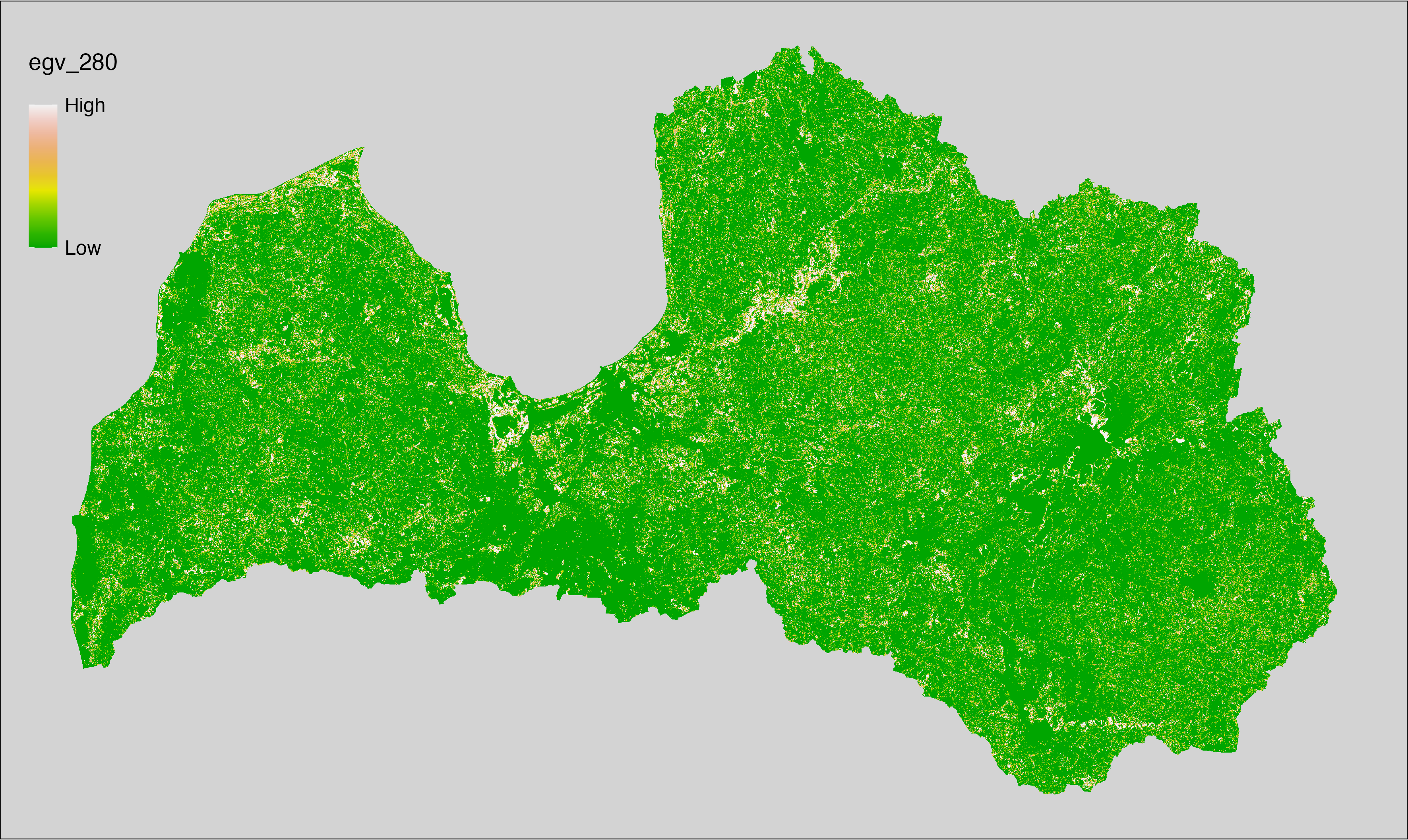
6.281 ForestsAge_Old_r500
filename: ForestsAge_Old_r500.tif
layername: egv_281
English name: Fractional cover of Old (over rotation age) Forest Stands within the 0.5 km landscape
Latvian name: Vecu (kopš cirtmeta) mežaudžu platības īpatsvars 0,5 km ainavā
Procedure: The cover fraction within a radius of 500 m around the analysis grid cell is
calculated as the area-weighted sum of the analysis cells inside the
buffer, using the workflow egvtools::radius_function(). During the calculation of the landscape metric,
inverse distance weighted (power = 2) gap filling on the output is applied
to ensure no missing values at the edges. Then the layer is rewritten to set
its name. Finally, the layer is standardised by subtracting the arithmetic
mean and dividing by the root mean squared error.
Code
# libs ----
if(!require(terra)) {install.packages("terra"); require(terra)}
if(!require(egvtools)) {remotes::install_github("aavotins/egvtools"); require(egvtools)}
# Templates -----
template100=rast("./Templates/TemplateRasters/LV100m_10km.tif")
# radii ----
radius_function(
kvadrati_path = "./Templates/TemplateGrids/tiles/",
radii_path = "./Templates/TemplateGridPoints/tiles/",
tikls100_path = "./Templates/TemplateGrids/tikls100_sauzeme.parquet",
template_path = "./Templates/TemplateRasters/LV100m_10km.tif",
input_layers = c("./RasterGrids_100m/2024/RAW/ForestsAge_Old_cell.tif"),
layer_prefixes = c("ForestsAge_Old"),
output_dir = "./RasterGrids_100m/2024/RAW/",
n_workers = 6,
radii = c("r500"),
radius_mode = "sparse",
extract_fun = "mean",
fill_missing = TRUE,
IDW_weight = 2,
future_max_size = 40 * 1024^3)
# ForestsAge_Old_r500.tif egv_281
slanis=rast("./RasterGrids_100m/2024/RAW/ForestsAge_Old_r500.tif")
names(slanis)="egv_281"
slanis2=project(slanis,template100)
writeRaster(slanis2,
"./RasterGrids_100m/2024/RAW/ForestsAge_Old_r500.tif",
overwrite=TRUE)
# standardisation ----
if(!require(terra)) {install.packages("terra"); require(terra)}
if(!require(tidyverse)) {install.packages("tidyverse"); require(tidyverse)}
nosaukums="ForestsAge_Old_r500.tif"
ielasisanas_cels=paste0("./RasterGrids_100m/2024/RAW/",nosaukums)
saglabasanas_cels=paste0("./RasterGrids_100m/2024/Scaled/",nosaukums)
slanis=rast(ielasisanas_cels)
videjais=global(slanis,fun="mean",na.rm=TRUE)
centrets=slanis-videjais[,1]
standartnovirze=terra::global(centrets,fun="rms",na.rm=TRUE)
merogots=centrets/standartnovirze[,1]
writeRaster(merogots,
filename=saglabasanas_cels,
overwrite=TRUE)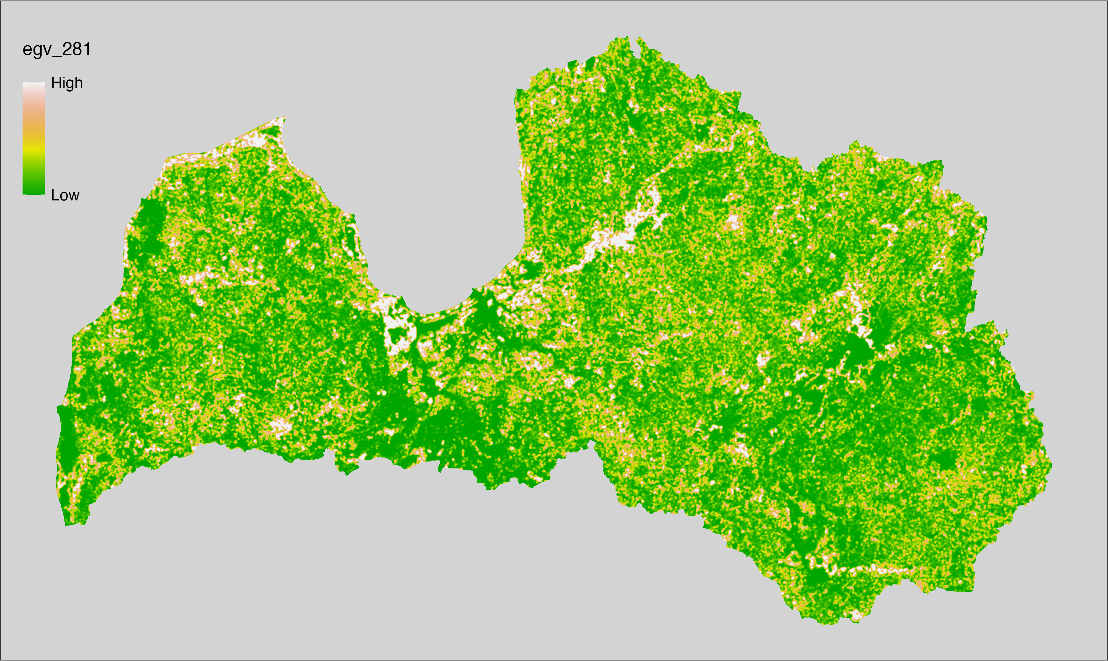
6.282 ForestsAge_Old_r1250
filename: ForestsAge_Old_r1250.tif
layername: egv_282
English name: Fractional cover of Old (over rotation age) Forest Stands within the 1.25 km landscape
Latvian name: Vecu (kopš cirtmeta) mežaudžu platības īpatsvars 1,25 km ainavā
Procedure: The cover fraction within a radius of 1250 m around the analysis grid cell
is calculated as the area-weighted sum of the analysis cells inside
the buffer, using the workflow egvtools::radius_function(). During the calculation of the landscape
metric, inverse distance weighted (power = 2) gap filling on the output is
applied to ensure no missing values at the edges. Then the layer is
rewritten to set its name. Finally, the layer is standardised by
subtracting the arithmetic mean and dividing by the root mean squared error.
Code
# libs ----
if(!require(terra)) {install.packages("terra"); require(terra)}
if(!require(egvtools)) {remotes::install_github("aavotins/egvtools"); require(egvtools)}
# Templates -----
template100=rast("./Templates/TemplateRasters/LV100m_10km.tif")
# radii ----
radius_function(
kvadrati_path = "./Templates/TemplateGrids/tiles/",
radii_path = "./Templates/TemplateGridPoints/tiles/",
tikls100_path = "./Templates/TemplateGrids/tikls100_sauzeme.parquet",
template_path = "./Templates/TemplateRasters/LV100m_10km.tif",
input_layers = c("./RasterGrids_100m/2024/RAW/ForestsAge_Old_cell.tif"),
layer_prefixes = c("ForestsAge_Old"),
output_dir = "./RasterGrids_100m/2024/RAW/",
n_workers = 6,
radii = c("r1250"),
radius_mode = "sparse",
extract_fun = "mean",
fill_missing = TRUE,
IDW_weight = 2,
future_max_size = 40 * 1024^3)
# ForestsAge_Old_r1250.tif egv_282
slanis=rast("./RasterGrids_100m/2024/RAW/ForestsAge_Old_r1250.tif")
names(slanis)="egv_282"
slanis2=project(slanis,template100)
writeRaster(slanis2,
"./RasterGrids_100m/2024/RAW/ForestsAge_Old_r1250.tif",
overwrite=TRUE)
# standardisation ----
if(!require(terra)) {install.packages("terra"); require(terra)}
if(!require(tidyverse)) {install.packages("tidyverse"); require(tidyverse)}
nosaukums="ForestsAge_Old_r1250.tif"
ielasisanas_cels=paste0("./RasterGrids_100m/2024/RAW/",nosaukums)
saglabasanas_cels=paste0("./RasterGrids_100m/2024/Scaled/",nosaukums)
slanis=rast(ielasisanas_cels)
videjais=global(slanis,fun="mean",na.rm=TRUE)
centrets=slanis-videjais[,1]
standartnovirze=terra::global(centrets,fun="rms",na.rm=TRUE)
merogots=centrets/standartnovirze[,1]
writeRaster(merogots,
filename=saglabasanas_cels,
overwrite=TRUE)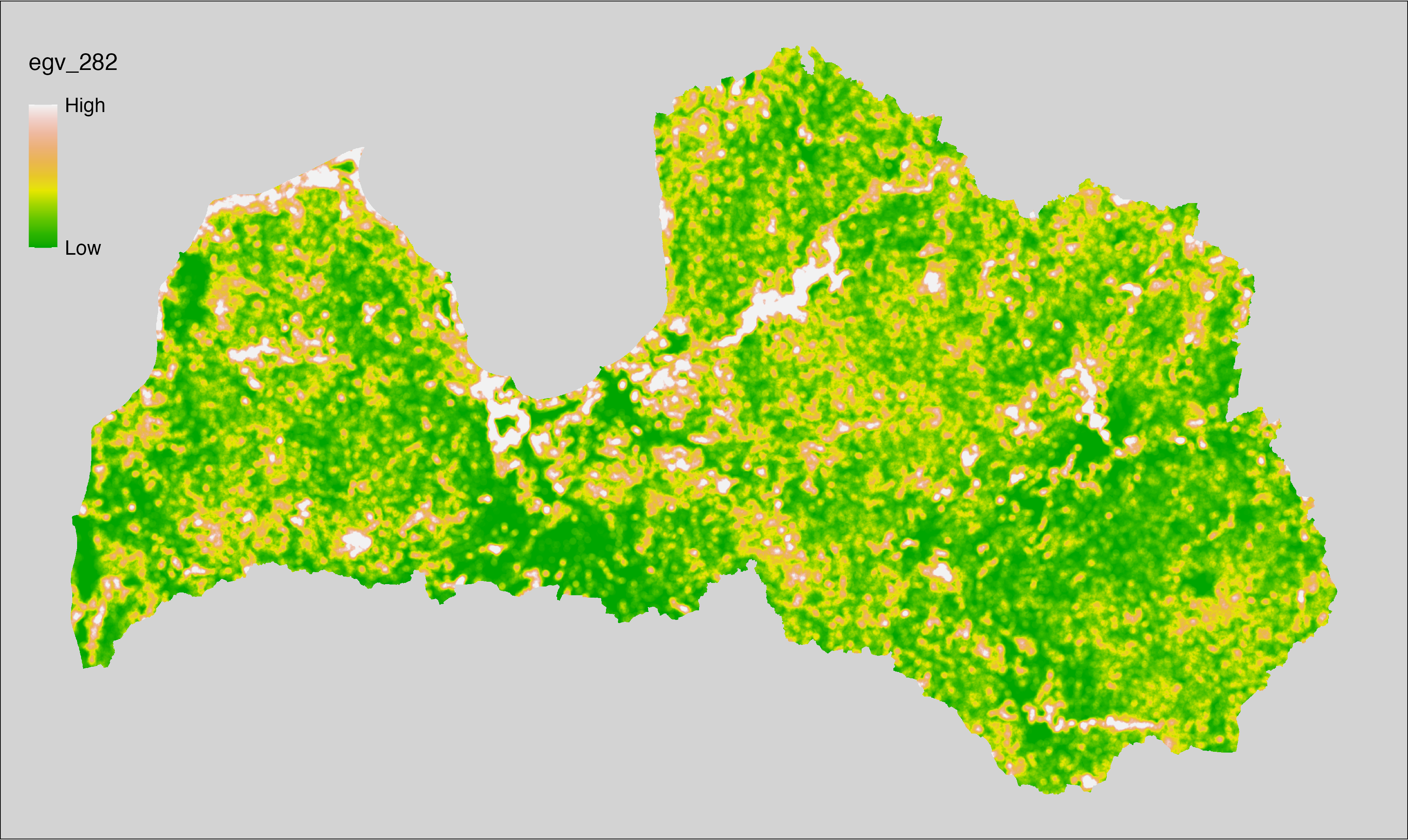
6.283 ForestsAge_Old_r3000
filename: ForestsAge_Old_r3000.tif
layername: egv_283
English name: Fractional cover of Old (over rotation age) Forest Stands within the 3 km landscape
Latvian name: Vecu (kopš cirtmeta) mežaudžu platības īpatsvars 3 km ainavā
Procedure: The cover fraction within a radius of 3000 m around the analysis grid cell
is calculated as the area-weighted sum of the analysis cells inside
the buffer, using the workflow egvtools::radius_function(). During the calculation of the landscape
metric, inverse distance weighted (power = 2) gap filling on the output is
applied to ensure no missing values at the edges. Then the layer is
rewritten to set its name. Finally, the layer is standardised by
subtracting the arithmetic mean and dividing by the root mean squared error.
Code
# libs ----
if(!require(terra)) {install.packages("terra"); require(terra)}
if(!require(egvtools)) {remotes::install_github("aavotins/egvtools"); require(egvtools)}
# Templates -----
template100=rast("./Templates/TemplateRasters/LV100m_10km.tif")
# radii ----
radius_function(
kvadrati_path = "./Templates/TemplateGrids/tiles/",
radii_path = "./Templates/TemplateGridPoints/tiles/",
tikls100_path = "./Templates/TemplateGrids/tikls100_sauzeme.parquet",
template_path = "./Templates/TemplateRasters/LV100m_10km.tif",
input_layers = c("./RasterGrids_100m/2024/RAW/ForestsAge_Old_cell.tif"),
layer_prefixes = c("ForestsAge_Old"),
output_dir = "./RasterGrids_100m/2024/RAW/",
n_workers = 6,
radii = c("r3000"),
radius_mode = "sparse",
extract_fun = "mean",
fill_missing = TRUE,
IDW_weight = 2,
future_max_size = 40 * 1024^3)
# ForestsAge_Old_r3000.tif egv_283
slanis=rast("./RasterGrids_100m/2024/RAW/ForestsAge_Old_r3000.tif")
names(slanis)="egv_283"
slanis2=project(slanis,template100)
writeRaster(slanis2,
"./RasterGrids_100m/2024/RAW/ForestsAge_Old_r3000.tif",
overwrite=TRUE)
# standardisation ----
if(!require(terra)) {install.packages("terra"); require(terra)}
if(!require(tidyverse)) {install.packages("tidyverse"); require(tidyverse)}
nosaukums="ForestsAge_Old_r3000.tif"
ielasisanas_cels=paste0("./RasterGrids_100m/2024/RAW/",nosaukums)
saglabasanas_cels=paste0("./RasterGrids_100m/2024/Scaled/",nosaukums)
slanis=rast(ielasisanas_cels)
videjais=global(slanis,fun="mean",na.rm=TRUE)
centrets=slanis-videjais[,1]
standartnovirze=terra::global(centrets,fun="rms",na.rm=TRUE)
merogots=centrets/standartnovirze[,1]
writeRaster(merogots,
filename=saglabasanas_cels,
overwrite=TRUE)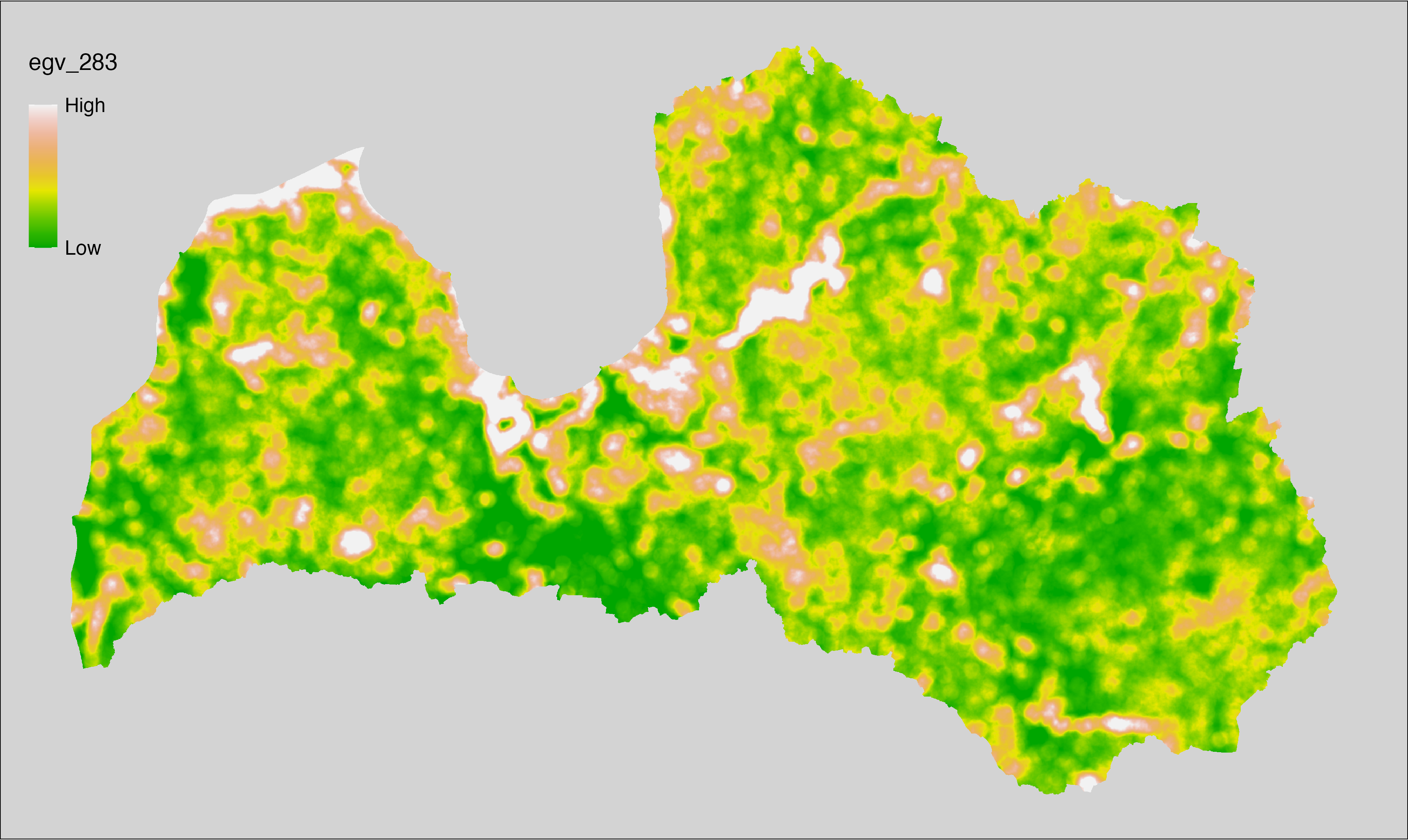
6.284 ForestsAge_Old_r10000
filename: ForestsAge_Old_r10000.tif
layername: egv_284
English name: Fractional cover of Old (over rotation age) Forest Stands within the 10 km landscape
Latvian name: Vecu (kopš cirtmeta) mežaudžu platības īpatsvars 10 km ainavā
Procedure: The cover fraction within a radius of 10000 m around the analysis grid cell
is calculated as the area-weighted sum of the analysis cells inside
the buffer, using the workflow egvtools::radius_function(). During the calculation of the landscape
metric, inverse distance weighted (power = 2) gap filling on the output is
applied to ensure no missing values at the edges. Then the layer is
rewritten to set its name. Finally, the layer is standardised by
subtracting the arithmetic mean and dividing by the root mean squared error.
Code
# libs ----
if(!require(terra)) {install.packages("terra"); require(terra)}
if(!require(egvtools)) {remotes::install_github("aavotins/egvtools"); require(egvtools)}
# Templates -----
template100=rast("./Templates/TemplateRasters/LV100m_10km.tif")
# radii ----
radius_function(
kvadrati_path = "./Templates/TemplateGrids/tiles/",
radii_path = "./Templates/TemplateGridPoints/tiles/",
tikls100_path = "./Templates/TemplateGrids/tikls100_sauzeme.parquet",
template_path = "./Templates/TemplateRasters/LV100m_10km.tif",
input_layers = c("./RasterGrids_100m/2024/RAW/ForestsAge_Old_cell.tif"),
layer_prefixes = c("ForestsAge_Old"),
output_dir = "./RasterGrids_100m/2024/RAW/",
n_workers = 6,
radii = c("r10000"),
radius_mode = "sparse",
extract_fun = "mean",
fill_missing = TRUE,
IDW_weight = 2,
future_max_size = 40 * 1024^3)
# ForestsAge_Old_r10000.tif egv_284
slanis=rast("./RasterGrids_100m/2024/RAW/ForestsAge_Old_r10000.tif")
names(slanis)="egv_284"
slanis2=project(slanis,template100)
writeRaster(slanis2,
"./RasterGrids_100m/2024/RAW/ForestsAge_Old_r10000.tif",
overwrite=TRUE)
# standardisation ----
if(!require(terra)) {install.packages("terra"); require(terra)}
if(!require(tidyverse)) {install.packages("tidyverse"); require(tidyverse)}
nosaukums="ForestsAge_Old_r10000.tif"
ielasisanas_cels=paste0("./RasterGrids_100m/2024/RAW/",nosaukums)
saglabasanas_cels=paste0("./RasterGrids_100m/2024/Scaled/",nosaukums)
slanis=rast(ielasisanas_cels)
videjais=global(slanis,fun="mean",na.rm=TRUE)
centrets=slanis-videjais[,1]
standartnovirze=terra::global(centrets,fun="rms",na.rm=TRUE)
merogots=centrets/standartnovirze[,1]
writeRaster(merogots,
filename=saglabasanas_cels,
overwrite=TRUE)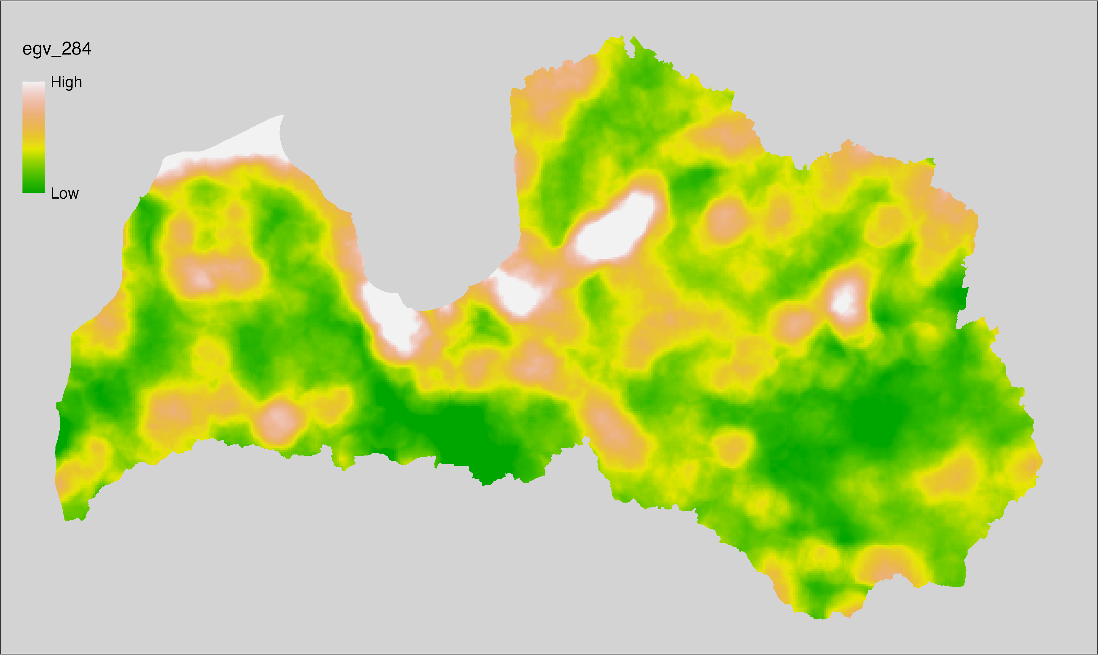
6.285 ForestsAge_YoungTallStandsShrubs_cell
filename: ForestsAge_YoungTallStandsShrubs_cell.tif
layername: egv_285
English name: Fractional cover of Shrubs, Young Forest Stands (at least 5 m tall) within the analysis cell (1 ha)
Latvian name: Krūmāju un jaunaudžu (no 5 m augstuma) platības īpatsvars analīzes šūnā (1 ha)
Procedure: Most EGVs describing forests are spatially restricted to areas outside of clearcuts and dead stands. This mask is created using a combination of the State Forest Service’s State Forest Registry land category 12 and 14, and The Global Forest Watch pixels classified as lost tree canopy cover since 2020 (raster layer matching input, presence = 1, absence = 0).
To prepare this
EGV, stands in land category 10 and age group 1 with height above 5 m are
selected from the State Forest Service’s State Forest Registry and
rasterised (presence = 1, NA otherwise). This layer is then combined with the category
620 from the Landscape classification (presence = 1, 0 otherwise).
Values in pixels matching the clearcut mask are set to 0. The resulting layer
is then aggregated to EGV resolution using the workflow egvtools::input2egv(), which
calculates the arithmetic mean to determine the cover fraction. During
aggregation, inverse distance weighted (power = 2) gap filling on the output is
applied to ensure no missing values at the edges. Finally, the layer is
standardised by subtracting the arithmetic mean and dividing by the root mean squared
error.
Code
# libs ----
if(!require(egvtools)) {remotes::install_github("aavotins/egvtools"); require(egvtools)}
if(!require(terra)) {install.packages("terra"); require(terra)}
if(!require(sf)) {install.packages("sf"); require(sf)}
if(!require(tidyverse)) {install.packages("tidyverse"); require(tidyverse)}
if(!require(sfarrow)) {install.packages("sfarrow"); require(sfarrow)}
if(!require(readxl)) {install.packages("readxl"); require(readxl)}
if(!require(raster)) {install.packages("raster"); require(raster)}
if(!require(fasterize)) {install.packages("fasterize"); require(fasterize)}
# templates ----
template100=rast("./Templates/TemplateRasters/LV100m_10km.tif")
template10=rast("./Templates/TemplateRasters/LV10m_10km.tif")
rastrs10=raster(template10)
nulls10=rast("./Templates/TemplateRasters/nulls_LV10m_10km.tif")
nulls100=rast("./Templates/TemplateRasters/nulls_LV100m_10km.tif")
# simple landscape ----
simple_landscape=rast("RasterGrids_10m/2024/Ainava_vienk_mask.tif")
# mvr ----
mvr=st_read_parquet("./Geodata/2024/MVR/nogabali_2024janv.parquet")
mvr$yes=1
# clear cut mask ----
izcirtumi=mvr %>%
filter(zkat %in% c("12","14")) %>%
dplyr::select(yes)
r_izcirtumi_mvr=fasterize(izcirtumi,rastrs10,field="yes")
t_izcirtumi_mvr=rast(r_izcirtumi_mvr)
plot(t_izcirtumi_mvr)
tcl=rast("./Geodata/2024/Trees/GFW/TreeCoverLoss_v1_12.tif")
tcl2=ifel(tcl<20,0,1)
tclX=cover(tcl2,nulls10)
plot(tclX)
clearcut_mask=cover(t_izcirtumi_mvr,tclX,
filename="./RasterGrids_10m/2024/Mask_clearcuts.tif",
overwrite=TRUE)
plot(clearcut_mask)
rm(izcirtumi)
rm(r_izcirtumi_mvr)
rm(t_izcirtumi_mvr)
rm(tcl)
rm(tcl2)
rm(tclX)
# ForestsAge_YoungTallStandsShrubs_cell.tif egv_285 ----
jaunasaugstas=mvr %>%
filter(zkat=="10") %>%
filter(h10>=5) %>%
filter(vgr %in% c("1")) %>%
dplyr::select(yes)
r_jaunasaugstas=fasterize(jaunasaugstas,rastrs10,field="yes")
t_jaunasaugstas=rast(r_jaunasaugstas)
plot(t_jaunasaugstas)
shrubs=ifel(simple_landscape==620,1,0)
younshrubs=cover(t_jaunasaugstas,shrubs)
plot(younshrubs)
younshrubs2=ifel(younshrubs==1&clearcut_mask==0,1,0)
plot(younshrubs2)
i2e_rez=egvtools::input2egv(input=younshrubs2,
egv_template= "./Templates/TemplateRasters/LV100m_10km.tif",
summary_function = "average",
missing_job = "FillOutput",
outlocation = "./RasterGrids_100m/2024/RAW/",
outfilename = "ForestsAge_YoungTallStandsShrubs_cell.tif",
layername = "egv_285",
idw_weight = 2,
plot_gaps = FALSE,plot_final = TRUE)
i2e_rez
rm(jaunasaugstas)
rm(r_jaunasaugstas)
rm(t_jaunasaugstas)
rm(shrubs)
rm(younshrubs)
rm(younshrubs2)
rm(i2e_rez)
# standardisation ----
if(!require(terra)) {install.packages("terra"); require(terra)}
if(!require(tidyverse)) {install.packages("tidyverse"); require(tidyverse)}
nosaukums="ForestsAge_YoungTallStandsShrubs_cell.tif"
ielasisanas_cels=paste0("./RasterGrids_100m/2024/RAW/",nosaukums)
saglabasanas_cels=paste0("./RasterGrids_100m/2024/Scaled/",nosaukums)
slanis=rast(ielasisanas_cels)
videjais=global(slanis,fun="mean",na.rm=TRUE)
centrets=slanis-videjais[,1]
standartnovirze=terra::global(centrets,fun="rms",na.rm=TRUE)
merogots=centrets/standartnovirze[,1]
writeRaster(merogots,
filename=saglabasanas_cels,
overwrite=TRUE)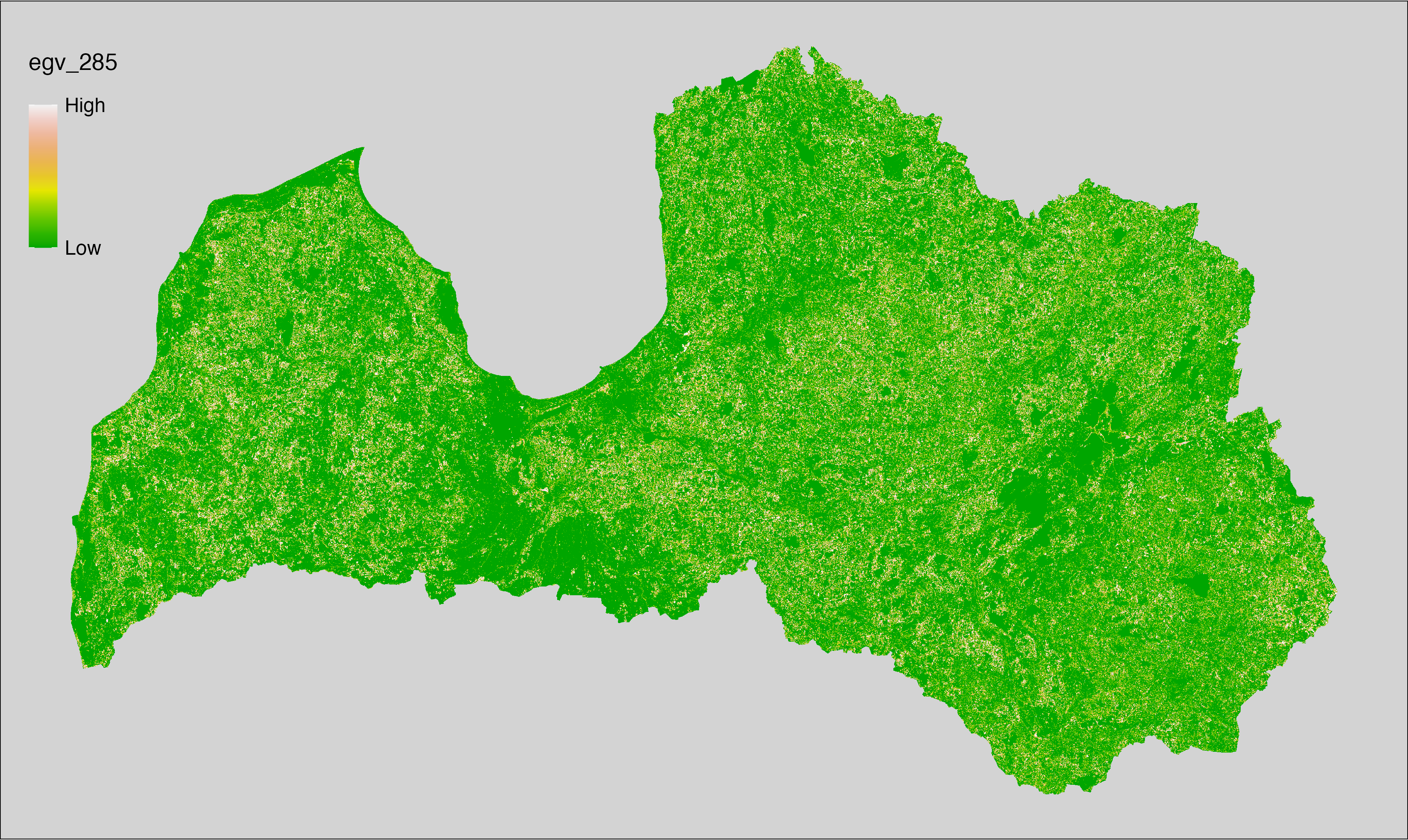
6.286 ForestsAge_YoungTallStandsShrubs_r500
filename: ForestsAge_YoungTallStandsShrubs_r500.tif
layername: egv_286
English name: Fractional cover of Shrubs, Young Forest Stands (at least 5 m tall) within the 0.5 km landscape
Latvian name: Krūmāju un jaunaudžu (no 5 m augstuma) platības īpatsvars 0,5 km ainavā
Procedure: The cover fraction within a radius of 500 m around the analysis grid cell is
calculated as the area-weighted sum of the analysis cells inside the
buffer, using the workflow egvtools::radius_function(). During the calculation of the landscape metric,
inverse distance weighted (power = 2) gap filling on the output is applied
to ensure no missing values at the edges. Then the layer is rewritten to set
its name. Finally, the layer is standardised by subtracting the arithmetic
mean and dividing by the root mean squared error.
Code
# libs ----
if(!require(terra)) {install.packages("terra"); require(terra)}
if(!require(egvtools)) {remotes::install_github("aavotins/egvtools"); require(egvtools)}
# Templates -----
template100=rast("./Templates/TemplateRasters/LV100m_10km.tif")
# radii ----
radius_function(
kvadrati_path = "./Templates/TemplateGrids/tiles/",
radii_path = "./Templates/TemplateGridPoints/tiles/",
tikls100_path = "./Templates/TemplateGrids/tikls100_sauzeme.parquet",
template_path = "./Templates/TemplateRasters/LV100m_10km.tif",
input_layers = c("./RasterGrids_100m/2024/RAW/ForestsAge_YoungTallStandsShrubs_cell.tif"),
layer_prefixes = c("ForestsAge_YoungTallStandsShrubs"),
output_dir = "./RasterGrids_100m/2024/RAW/",
n_workers = 6,
radii = c("r500"),
radius_mode = "sparse",
extract_fun = "mean",
fill_missing = TRUE,
IDW_weight = 2,
future_max_size = 40 * 1024^3)
# ForestsAge_YoungTallStandsShrubs_r500.tif egv_286
slanis=rast("./RasterGrids_100m/2024/RAW/ForestsAge_YoungTallStandsShrubs_r500.tif")
names(slanis)="egv_286"
slanis2=project(slanis,template100)
writeRaster(slanis2,
"./RasterGrids_100m/2024/RAW/ForestsAge_YoungTallStandsShrubs_r500.tif",
overwrite=TRUE)
# standardisation ----
if(!require(terra)) {install.packages("terra"); require(terra)}
if(!require(tidyverse)) {install.packages("tidyverse"); require(tidyverse)}
nosaukums="ForestsAge_YoungTallStandsShrubs_r500.tif"
ielasisanas_cels=paste0("./RasterGrids_100m/2024/RAW/",nosaukums)
saglabasanas_cels=paste0("./RasterGrids_100m/2024/Scaled/",nosaukums)
slanis=rast(ielasisanas_cels)
videjais=global(slanis,fun="mean",na.rm=TRUE)
centrets=slanis-videjais[,1]
standartnovirze=terra::global(centrets,fun="rms",na.rm=TRUE)
merogots=centrets/standartnovirze[,1]
writeRaster(merogots,
filename=saglabasanas_cels,
overwrite=TRUE)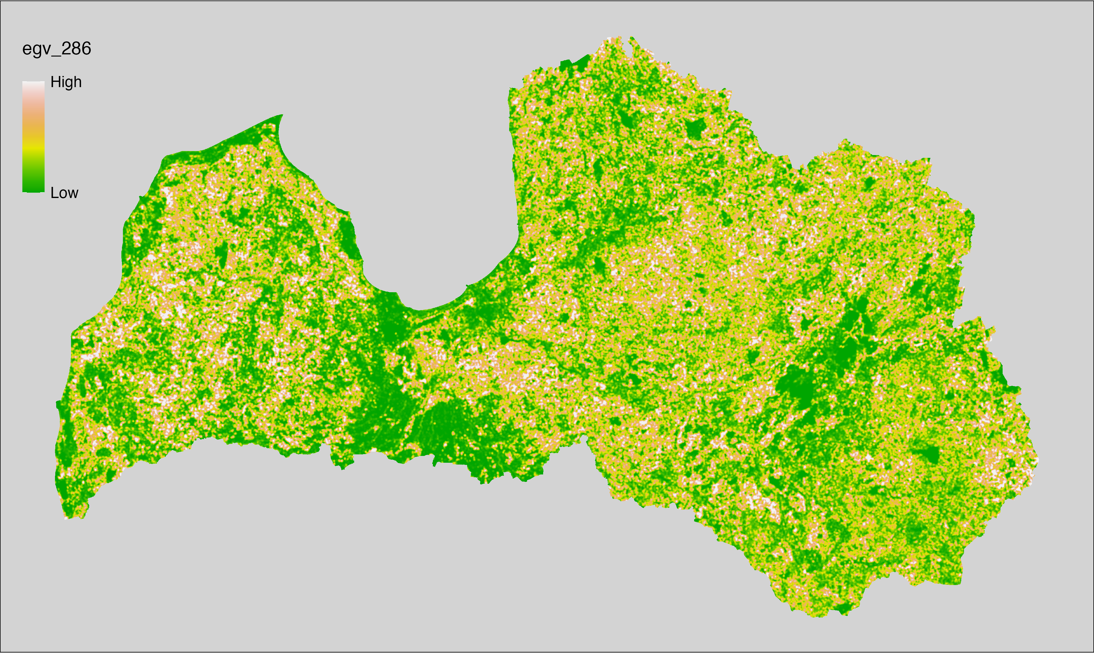
6.287 ForestsAge_YoungTallStandsShrubs_r1250
filename: ForestsAge_YoungTallStandsShrubs_r1250.tif
layername: egv_287
English name: Fractional cover of Shrubs, Young Forest Stands (at least 5 m tall) within the 1.25 km landscape
Latvian name: Krūmāju un jaunaudžu (no 5 m augstuma) platības īpatsvars 1,25 km ainavā
Procedure: The cover fraction within a radius of 1250 m around the analysis grid cell
is calculated as the area-weighted sum of the analysis cells inside
the buffer, using the workflow egvtools::radius_function(). During the calculation of the landscape
metric, inverse distance weighted (power = 2) gap filling on the output is
applied to ensure no missing values at the edges. Then the layer is
rewritten to set its name. Finally, the layer is standardised by
subtracting the arithmetic mean and dividing by the root mean squared error.
Code
# libs ----
if(!require(terra)) {install.packages("terra"); require(terra)}
if(!require(egvtools)) {remotes::install_github("aavotins/egvtools"); require(egvtools)}
# Templates -----
template100=rast("./Templates/TemplateRasters/LV100m_10km.tif")
# radii ----
radius_function(
kvadrati_path = "./Templates/TemplateGrids/tiles/",
radii_path = "./Templates/TemplateGridPoints/tiles/",
tikls100_path = "./Templates/TemplateGrids/tikls100_sauzeme.parquet",
template_path = "./Templates/TemplateRasters/LV100m_10km.tif",
input_layers = c("./RasterGrids_100m/2024/RAW/ForestsAge_YoungTallStandsShrubs_cell.tif"),
layer_prefixes = c("ForestsAge_YoungTallStandsShrubs"),
output_dir = "./RasterGrids_100m/2024/RAW/",
n_workers = 6,
radii = c("r1250"),
radius_mode = "sparse",
extract_fun = "mean",
fill_missing = TRUE,
IDW_weight = 2,
future_max_size = 40 * 1024^3)
# ForestsAge_YoungTallStandsShrubs_r1250.tif egv_287
slanis=rast("./RasterGrids_100m/2024/RAW/ForestsAge_YoungTallStandsShrubs_r1250.tif")
names(slanis)="egv_287"
slanis2=project(slanis,template100)
writeRaster(slanis2,
"./RasterGrids_100m/2024/RAW/ForestsAge_YoungTallStandsShrubs_r1250.tif",
overwrite=TRUE)
# standardisation ----
if(!require(terra)) {install.packages("terra"); require(terra)}
if(!require(tidyverse)) {install.packages("tidyverse"); require(tidyverse)}
nosaukums="ForestsAge_YoungTallStandsShrubs_r1250.tif"
ielasisanas_cels=paste0("./RasterGrids_100m/2024/RAW/",nosaukums)
saglabasanas_cels=paste0("./RasterGrids_100m/2024/Scaled/",nosaukums)
slanis=rast(ielasisanas_cels)
videjais=global(slanis,fun="mean",na.rm=TRUE)
centrets=slanis-videjais[,1]
standartnovirze=terra::global(centrets,fun="rms",na.rm=TRUE)
merogots=centrets/standartnovirze[,1]
writeRaster(merogots,
filename=saglabasanas_cels,
overwrite=TRUE)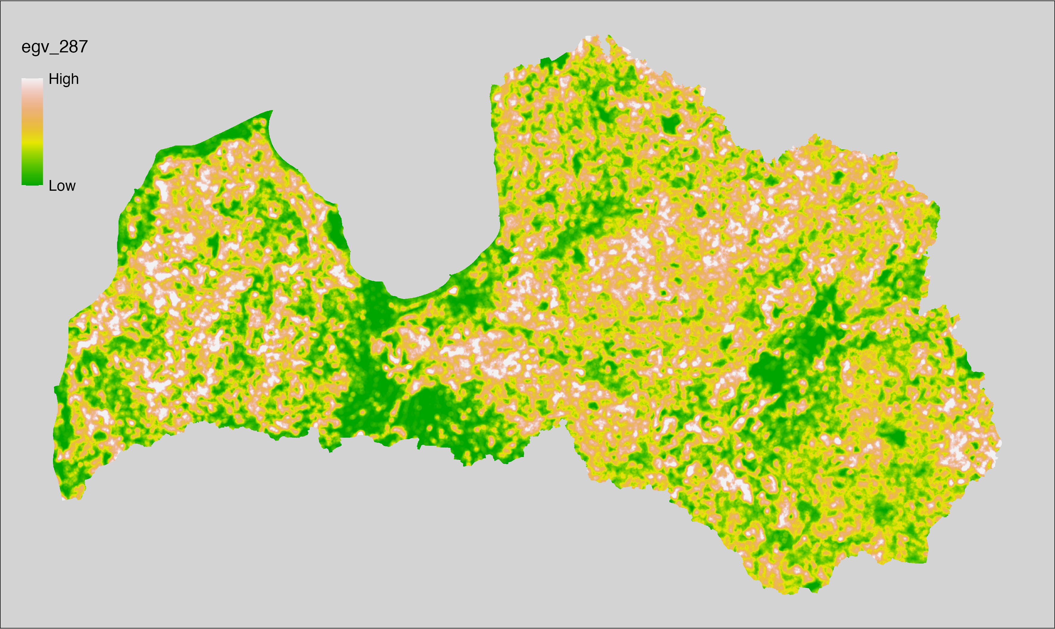
6.288 ForestsAge_YoungTallStandsShrubs_r3000
filename: ForestsAge_YoungTallStandsShrubs_r3000.tif
layername: egv_288
English name: Fractional cover of Shrubs, Young Forest Stands (at least 5 m tall) within the 3 km landscape
Latvian name: Krūmāju un jaunaudžu (no 5 m augstuma) platības īpatsvars 3 km ainavā
Procedure: The cover fraction within a radius of 3000 m around the analysis grid cell
is calculated as the area-weighted sum of the analysis cells inside
the buffer, using the workflow egvtools::radius_function(). During the calculation of the landscape
metric, inverse distance weighted (power = 2) gap filling on the output is
applied to ensure no missing values at the edges. Then the layer is
rewritten to set its name. Finally, the layer is standardised by
subtracting the arithmetic mean and dividing by the root mean squared error.
Code
# libs ----
if(!require(terra)) {install.packages("terra"); require(terra)}
if(!require(egvtools)) {remotes::install_github("aavotins/egvtools"); require(egvtools)}
# Templates -----
template100=rast("./Templates/TemplateRasters/LV100m_10km.tif")
# radii ----
radius_function(
kvadrati_path = "./Templates/TemplateGrids/tiles/",
radii_path = "./Templates/TemplateGridPoints/tiles/",
tikls100_path = "./Templates/TemplateGrids/tikls100_sauzeme.parquet",
template_path = "./Templates/TemplateRasters/LV100m_10km.tif",
input_layers = c("./RasterGrids_100m/2024/RAW/ForestsAge_YoungTallStandsShrubs_cell.tif"),
layer_prefixes = c("ForestsAge_YoungTallStandsShrubs"),
output_dir = "./RasterGrids_100m/2024/RAW/",
n_workers = 6,
radii = c("r3000"),
radius_mode = "sparse",
extract_fun = "mean",
fill_missing = TRUE,
IDW_weight = 2,
future_max_size = 40 * 1024^3)
# ForestsAge_YoungTallStandsShrubs_r3000.tif egv_288
slanis=rast("./RasterGrids_100m/2024/RAW/ForestsAge_YoungTallStandsShrubs_r3000.tif")
names(slanis)="egv_288"
slanis2=project(slanis,template100)
writeRaster(slanis2,
"./RasterGrids_100m/2024/RAW/ForestsAge_YoungTallStandsShrubs_r3000.tif",
overwrite=TRUE)
# standardisation ----
if(!require(terra)) {install.packages("terra"); require(terra)}
if(!require(tidyverse)) {install.packages("tidyverse"); require(tidyverse)}
nosaukums="ForestsAge_YoungTallStandsShrubs_r3000.tif"
ielasisanas_cels=paste0("./RasterGrids_100m/2024/RAW/",nosaukums)
saglabasanas_cels=paste0("./RasterGrids_100m/2024/Scaled/",nosaukums)
slanis=rast(ielasisanas_cels)
videjais=global(slanis,fun="mean",na.rm=TRUE)
centrets=slanis-videjais[,1]
standartnovirze=terra::global(centrets,fun="rms",na.rm=TRUE)
merogots=centrets/standartnovirze[,1]
writeRaster(merogots,
filename=saglabasanas_cels,
overwrite=TRUE)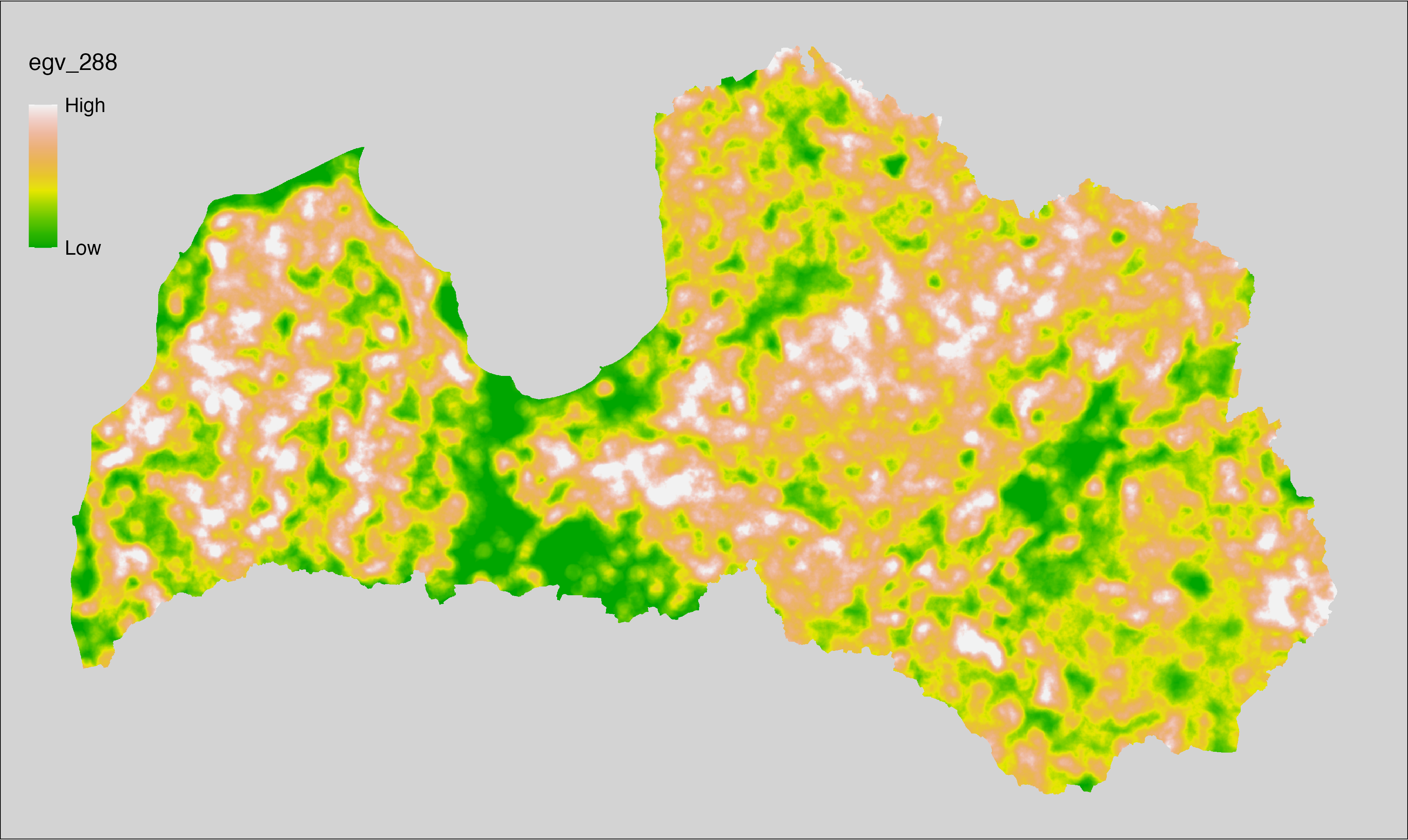
6.289 ForestsAge_YoungTallStandsShrubs_r10000
filename: ForestsAge_YoungTallStandsShrubs_r10000.tif
layername: egv_289
English name: Fractional cover of Shrubs, Young Forest Stands (at least 5 m tall) within the 10 km landscape
Latvian name: Krūmāju un jaunaudžu (no 5 m augstuma) platības īpatsvars 10 km ainavā
Procedure: The cover fraction within a radius of 10000 m around the analysis grid cell
is calculated as the area-weighted sum of the analysis cells inside
the buffer, using the workflow egvtools::radius_function(). During the calculation of the landscape
metric, inverse distance weighted (power = 2) gap filling on the output is
applied to ensure no missing values at the edges. Then the layer is
rewritten to set its name. Finally, the layer is standardised by
subtracting the arithmetic mean and dividing by the root mean squared error.
Code
# libs ----
if(!require(terra)) {install.packages("terra"); require(terra)}
if(!require(egvtools)) {remotes::install_github("aavotins/egvtools"); require(egvtools)}
# Templates -----
template100=rast("./Templates/TemplateRasters/LV100m_10km.tif")
# radii ----
radius_function(
kvadrati_path = "./Templates/TemplateGrids/tiles/",
radii_path = "./Templates/TemplateGridPoints/tiles/",
tikls100_path = "./Templates/TemplateGrids/tikls100_sauzeme.parquet",
template_path = "./Templates/TemplateRasters/LV100m_10km.tif",
input_layers = c("./RasterGrids_100m/2024/RAW/ForestsAge_YoungTallStandsShrubs_cell.tif"),
layer_prefixes = c("ForestsAge_YoungTallStandsShrubs"),
output_dir = "./RasterGrids_100m/2024/RAW/",
n_workers = 6,
radii = c("r10000"),
radius_mode = "sparse",
extract_fun = "mean",
fill_missing = TRUE,
IDW_weight = 2,
future_max_size = 40 * 1024^3)
# ForestsAge_YoungTallStandsShrubs_r10000.tif egv_289
slanis=rast("./RasterGrids_100m/2024/RAW/ForestsAge_YoungTallStandsShrubs_r10000.tif")
names(slanis)="egv_289"
slanis2=project(slanis,template100)
writeRaster(slanis2,
"./RasterGrids_100m/2024/RAW/ForestsAge_YoungTallStandsShrubs_r10000.tif",
overwrite=TRUE)
# standardisation ----
if(!require(terra)) {install.packages("terra"); require(terra)}
if(!require(tidyverse)) {install.packages("tidyverse"); require(tidyverse)}
nosaukums="ForestsAge_YoungTallStandsShrubs_r10000.tif"
ielasisanas_cels=paste0("./RasterGrids_100m/2024/RAW/",nosaukums)
saglabasanas_cels=paste0("./RasterGrids_100m/2024/Scaled/",nosaukums)
slanis=rast(ielasisanas_cels)
videjais=global(slanis,fun="mean",na.rm=TRUE)
centrets=slanis-videjais[,1]
standartnovirze=terra::global(centrets,fun="rms",na.rm=TRUE)
merogots=centrets/standartnovirze[,1]
writeRaster(merogots,
filename=saglabasanas_cels,
overwrite=TRUE)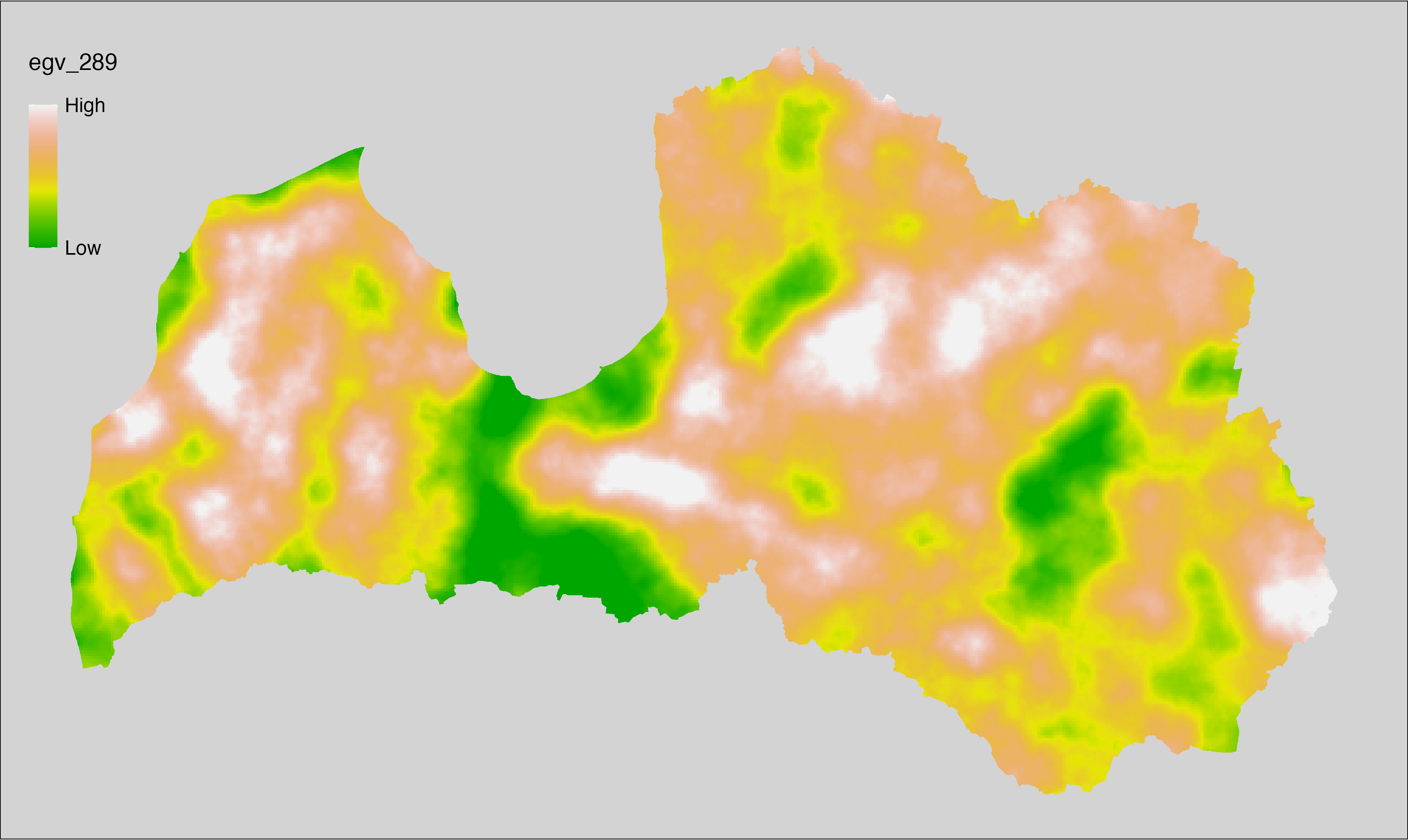
6.290 ForestsQuant_AgeProp-average_cell
filename: ForestsQuant_AgeProp-average_cell.tif
layername: egv_290
English name: Average stand age relative to rotation age within the analysis cell (1 ha)
Latvian name: Mežaudzes vecuma attiecība pret cirtmetu, vidējais analīzes šūnā (1 ha)
Procedure: Most EGVs describing forests are spatially restricted to areas outside of clearcuts and dead stands. This mask is created using a combination of the State Forest Service’s State Forest Registry land category 12 and 14, and The Global Forest Watch pixels classified as lost tree canopy cover since 2020 (raster layer matching input, presence = 1, absence = 0).
To prepare this EGV, every forest stand had assigned legal rotation age, based on dominant tree species and bonity class as registered in the State Forest Service’s State Forest Registry. We assumed 35 years as the rotation age for grey alder. The registered age of the dominant tree group is then divided by the stand specific legal rotation age. This attribute has some extreme values. We chose to limit them to the nearest integer showing only minimal accumulation in histogram.
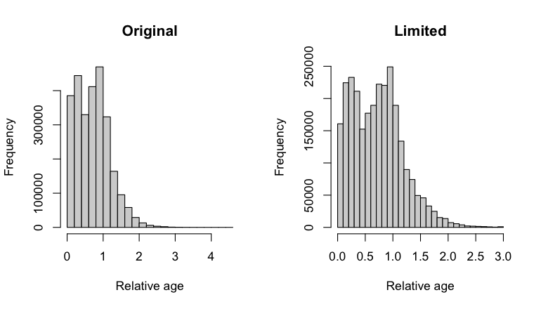
Resulting values at polygon geometries are rasterised with the workflow
egvtools::polygon2input(), restricting to pixels outside the clearcut mask. No
background values are assigned during rasterisation. The resulting layer is
then aggregated to EGV resolution using the workflow egvtools::input2egv() by calculating
arithmetic mean. After the aggregation, cells with no forest information are
filled with value 0. Finally, the layer is standardised by subtracting
the arithmetic mean and dividing by the root mean squared error.
Code
# libs ----
if(!require(egvtools)) {remotes::install_github("aavotins/egvtools"); require(egvtools)}
if(!require(terra)) {install.packages("terra"); require(terra)}
if(!require(sf)) {install.packages("sf"); require(sf)}
if(!require(tidyverse)) {install.packages("tidyverse"); require(tidyverse)}
if(!require(sfarrow)) {install.packages("sfarrow"); require(sfarrow)}
if(!require(readxl)) {install.packages("readxl"); require(readxl)}
if(!require(raster)) {install.packages("raster"); require(raster)}
if(!require(fasterize)) {install.packages("fasterize"); require(fasterize)}
# templates ----
template100=rast("./Templates/TemplateRasters/LV100m_10km.tif")
template10=rast("./Templates/TemplateRasters/LV10m_10km.tif")
rastrs10=raster(template10)
nulls10=rast("./Templates/TemplateRasters/nulls_LV10m_10km.tif")
nulls100=rast("./Templates/TemplateRasters/nulls_LV100m_10km.tif")
# simple landscape ----
simple_landscape=rast("RasterGrids_10m/2024/Ainava_vienk_mask.tif")
# mvr ----
mvr=st_read_parquet("./Geodata/2024/MVR/nogabali_2024janv.parquet")
mvr$yes=1
# clear cut mask ----
izcirtumi=mvr %>%
filter(zkat %in% c("12","14")) %>%
dplyr::select(yes)
r_izcirtumi_mvr=fasterize(izcirtumi,rastrs10,field="yes")
t_izcirtumi_mvr=rast(r_izcirtumi_mvr)
plot(t_izcirtumi_mvr)
tcl=rast("./Geodata/2024/Trees/GFW/TreeCoverLoss_v1_12.tif")
tcl2=ifel(tcl<20,0,1)
tclX=cover(tcl2,nulls10)
plot(tclX)
clearcut_mask=cover(t_izcirtumi_mvr,tclX,
filename="./RasterGrids_10m/2024/Mask_clearcuts.tif",
overwrite=TRUE)
plot(clearcut_mask)
rm(izcirtumi)
rm(r_izcirtumi_mvr)
rm(t_izcirtumi_mvr)
rm(tcl)
rm(tcl2)
rm(tclX)
# ForestsQuant_AgeProp-average_cell.tif egv_290 ----
#Forest law https://likumi.lv/ta/id/2825#p9
ozoli=c("10","61")
priedes_lapegles=c("1","13","14","22")
eolgvk=c("3","15","23","11","64","12","62","16","65","24","63")
berzi=c("4")
melnalksni=c("6")
apses=c("8","19","68")
bonA=c("0","1")
bonB=c("2","3")
bonC=c("4","5","6")
bonAB=c("0","1","2","3")
nogabali=mvr %>%
mutate(cirtmets=ifelse((s10 %in% ozoli)&(bon %in% bonA),101,
ifelse((s10 %in% ozoli),121,NA))) %>%
mutate(cirtmets=ifelse((s10 %in% priedes_lapegles)&(bon %in% bonAB),101,
ifelse((s10 %in% priedes_lapegles),121,cirtmets))) %>%
mutate(cirtmets=ifelse((s10 %in% eolgvk),81,cirtmets)) %>%
mutate(cirtmets=ifelse((s10 %in% berzi)&(bon %in% bonAB),71,
ifelse((s10 %in% berzi),51,cirtmets))) %>%
mutate(cirtmets=ifelse((s10 %in% melnalksni),71,cirtmets)) %>%
mutate(cirtmets=ifelse((s10 %in% apses),41,cirtmets)) %>%
mutate(cirtmets=ifelse(is.na(cirtmets)&zkat=="10",35,cirtmets)) %>%
mutate(nogvec=a10/cirtmets) %>%
mutate(nogvec2=ifelse(nogvec>3,3,nogvec)) %>%
filter(!is.na(nogvec2))
par(mfrow=c(1,2))
options(scipen=999)
hist(nogabali$nogvec,main="Original",xlab="Relative age")
hist(nogabali$nogvec2,main="Limited",xlab="Relative age")
par(mfrow=c(1,1))
options(scipen=0)
# 700*400
p2i_rez=polygon2input(vector_data=nogabali,
template_path = "./Templates/TemplateRasters/LV10m_10km.tif",
out_path = "./RasterGrids_10m/2024/",
file_name = "ForestQuant_AgeProp.tif",
value_field = "nogvec2",
fun="max",
prepare=FALSE,
restrict_to = clearcut_mask,
restrict_values = 0,
plot_result=TRUE)
p2i_rez
i2e_rez=input2egv(input="./RasterGrids_10m/2024/ForestQuant_AgeProp.tif",
egv_template = "./Templates/TemplateRasters/LV100m_10km.tif",
summary_function = "average",
missing_job = "CoverOutput",
output_bg = "./Templates/TemplateRasters/nulls_LV100m_10km.tif",
outlocation = "./RasterGrids_100m/2024/RAW/",
outfilename = "ForestsQuant_AgeProp-average_cell.tif",
layername = "egv_290",
plot_final=TRUE)
i2e_rez
rm(nogabali)
rm(p2i_rez)
rm(i2e_rez)
unlink("./RasterGrids_10m/2024/ForestQuant_AgeProp.tif")
# standardisation ----
if(!require(terra)) {install.packages("terra"); require(terra)}
if(!require(tidyverse)) {install.packages("tidyverse"); require(tidyverse)}
nosaukums="ForestsQuant_AgeProp-average_cell.tif"
ielasisanas_cels=paste0("./RasterGrids_100m/2024/RAW/",nosaukums)
saglabasanas_cels=paste0("./RasterGrids_100m/2024/Scaled/",nosaukums)
slanis=rast(ielasisanas_cels)
videjais=global(slanis,fun="mean",na.rm=TRUE)
centrets=slanis-videjais[,1]
standartnovirze=terra::global(centrets,fun="rms",na.rm=TRUE)
merogots=centrets/standartnovirze[,1]
writeRaster(merogots,
filename=saglabasanas_cels,
overwrite=TRUE)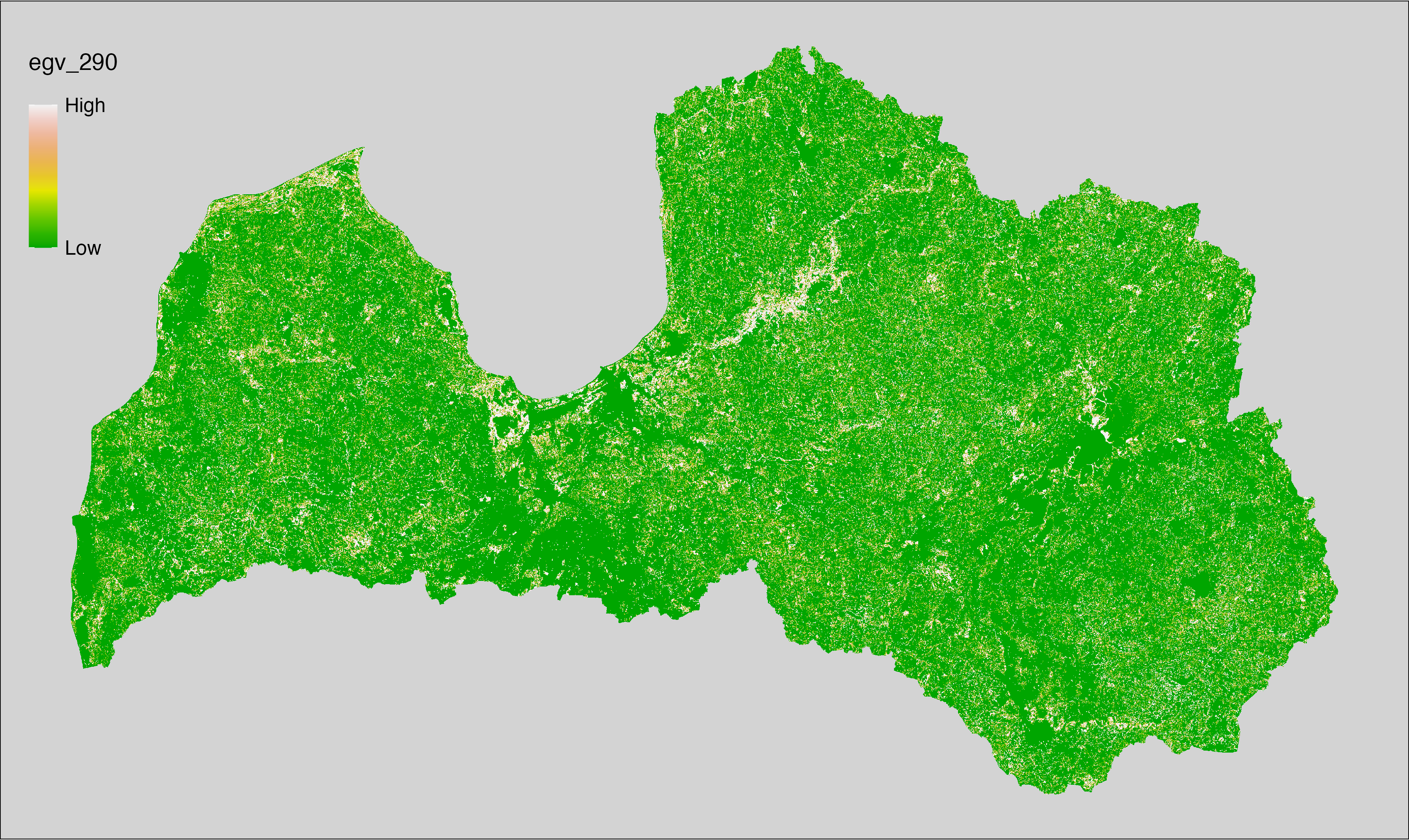
6.291 ForestsQuant_DominantDiameter-max_cell
filename: ForestsQuant_DominantDiameter-max_cell.tif
layername: egv_291
English name: Dominant tree trunk diameter, maximum within the analysis cell (1 ha)
Latvian name: Koku stumbra diametrs, valdaudzes maksimālais analīzes šūnā (1 ha)
Procedure: Most of forests describing EGVs are spatially restricted outside clearcuts and dead stands. Mask for this is created from the State Forest Service’s State Forest Registry land category 12 and 14 combined with The Global Forest Watch pixels classified as lost tree canopy cover since 2020 (raster layer matching input, presence = 1, absence = 0).
This EGV is prepared based on the information of dominant tree species per inventoried forest stand - State Forest Service’s State Forest Registry. This attribute has some extreme values. We chose to limit them to the nearest integer showing only minimal accumulation in histogram.
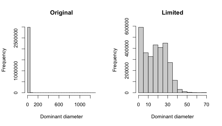
Resulting values at polygon geometries are rasterised with the workflow
egvtools::polygon2input(), restricting to pixels outside the clearcut mask. No
background values are assigned during rasterisation. The resulting layer is
then aggregated to EGV resolution using the workflow egvtools::input2egv() by calculating
maximum value. After the aggregation, cells with no forest information are
filled with value 0. Finally, the layer is standardised by subtracting
the arithmetic mean and dividing by the root mean squared error.
Code
# libs ----
if(!require(egvtools)) {remotes::install_github("aavotins/egvtools"); require(egvtools)}
if(!require(terra)) {install.packages("terra"); require(terra)}
if(!require(sf)) {install.packages("sf"); require(sf)}
if(!require(tidyverse)) {install.packages("tidyverse"); require(tidyverse)}
if(!require(sfarrow)) {install.packages("sfarrow"); require(sfarrow)}
if(!require(readxl)) {install.packages("readxl"); require(readxl)}
if(!require(raster)) {install.packages("raster"); require(raster)}
if(!require(fasterize)) {install.packages("fasterize"); require(fasterize)}
# templates ----
template100=rast("./Templates/TemplateRasters/LV100m_10km.tif")
template10=rast("./Templates/TemplateRasters/LV10m_10km.tif")
rastrs10=raster(template10)
nulls10=rast("./Templates/TemplateRasters/nulls_LV10m_10km.tif")
nulls100=rast("./Templates/TemplateRasters/nulls_LV100m_10km.tif")
# simple landscape ----
simple_landscape=rast("RasterGrids_10m/2024/Ainava_vienk_mask.tif")
# mvr ----
mvr=st_read_parquet("./Geodata/2024/MVR/nogabali_2024janv.parquet")
mvr$yes=1
# clear cut mask ----
izcirtumi=mvr %>%
filter(zkat %in% c("12","14")) %>%
dplyr::select(yes)
r_izcirtumi_mvr=fasterize(izcirtumi,rastrs10,field="yes")
t_izcirtumi_mvr=rast(r_izcirtumi_mvr)
plot(t_izcirtumi_mvr)
tcl=rast("./Geodata/2024/Trees/GFW/TreeCoverLoss_v1_12.tif")
tcl2=ifel(tcl<20,0,1)
tclX=cover(tcl2,nulls10)
plot(tclX)
clearcut_mask=cover(t_izcirtumi_mvr,tclX,
filename="./RasterGrids_10m/2024/Mask_clearcuts.tif",
overwrite=TRUE)
plot(clearcut_mask)
rm(izcirtumi)
rm(r_izcirtumi_mvr)
rm(t_izcirtumi_mvr)
rm(tcl)
rm(tcl2)
rm(tclX)
# ForestsQuant_DominantDiameter-max_cell.tif egv_291 ----
nogabali=mvr %>%
mutate(valddiam=ifelse(d10>70,70,d10)) %>%
filter(!is.na(valddiam))
par(mfrow=c(1,2))
options(scipen=999)
hist(nogabali$d10,main="Original",xlab="Dominant diameter")
hist(nogabali$valddiam,main="Limited",xlab="Dominant diameter")
par(mfrow=c(1,1))
options(scipen=0)
p2i_rez=polygon2input(vector_data=nogabali,
template_path = "./Templates/TemplateRasters/LV10m_10km.tif",
out_path = "./RasterGrids_10m/2024/",
file_name = "ForestQuant_DominantDiameter.tif",
value_field = "valddiam",
fun="max",
prepare=FALSE,
restrict_to = clearcut_mask,
restrict_values = 0,
plot_result=TRUE,
overwrite=TRUE)
p2i_rez
i2e_rez=input2egv(input="./RasterGrids_10m/2024/ForestQuant_DominantDiameter.tif",
egv_template = "./Templates/TemplateRasters/LV100m_10km.tif",
summary_function = "max",
missing_job = "CoverOutput",
output_bg = "./Templates/TemplateRasters/nulls_LV100m_10km.tif",
outlocation = "./RasterGrids_100m/2024/RAW/",
outfilename = "ForestsQuant_DominantDiameter-max_cell.tif",
layername = "egv_291",
plot_final=TRUE)
i2e_rez
rm(p2i_rez)
rm(nogabali)
rm(i2e_rez)
unlink("./RasterGrids_10m/2024/ForestQuant_DominantDiameter.tif")
# standardisation ----
if(!require(terra)) {install.packages("terra"); require(terra)}
if(!require(tidyverse)) {install.packages("tidyverse"); require(tidyverse)}
nosaukums="ForestsQuant_DominantDiameter-max_cell.tif"
ielasisanas_cels=paste0("./RasterGrids_100m/2024/RAW/",nosaukums)
saglabasanas_cels=paste0("./RasterGrids_100m/2024/Scaled/",nosaukums)
slanis=rast(ielasisanas_cels)
videjais=global(slanis,fun="mean",na.rm=TRUE)
centrets=slanis-videjais[,1]
standartnovirze=terra::global(centrets,fun="rms",na.rm=TRUE)
merogots=centrets/standartnovirze[,1]
writeRaster(merogots,
filename=saglabasanas_cels,
overwrite=TRUE)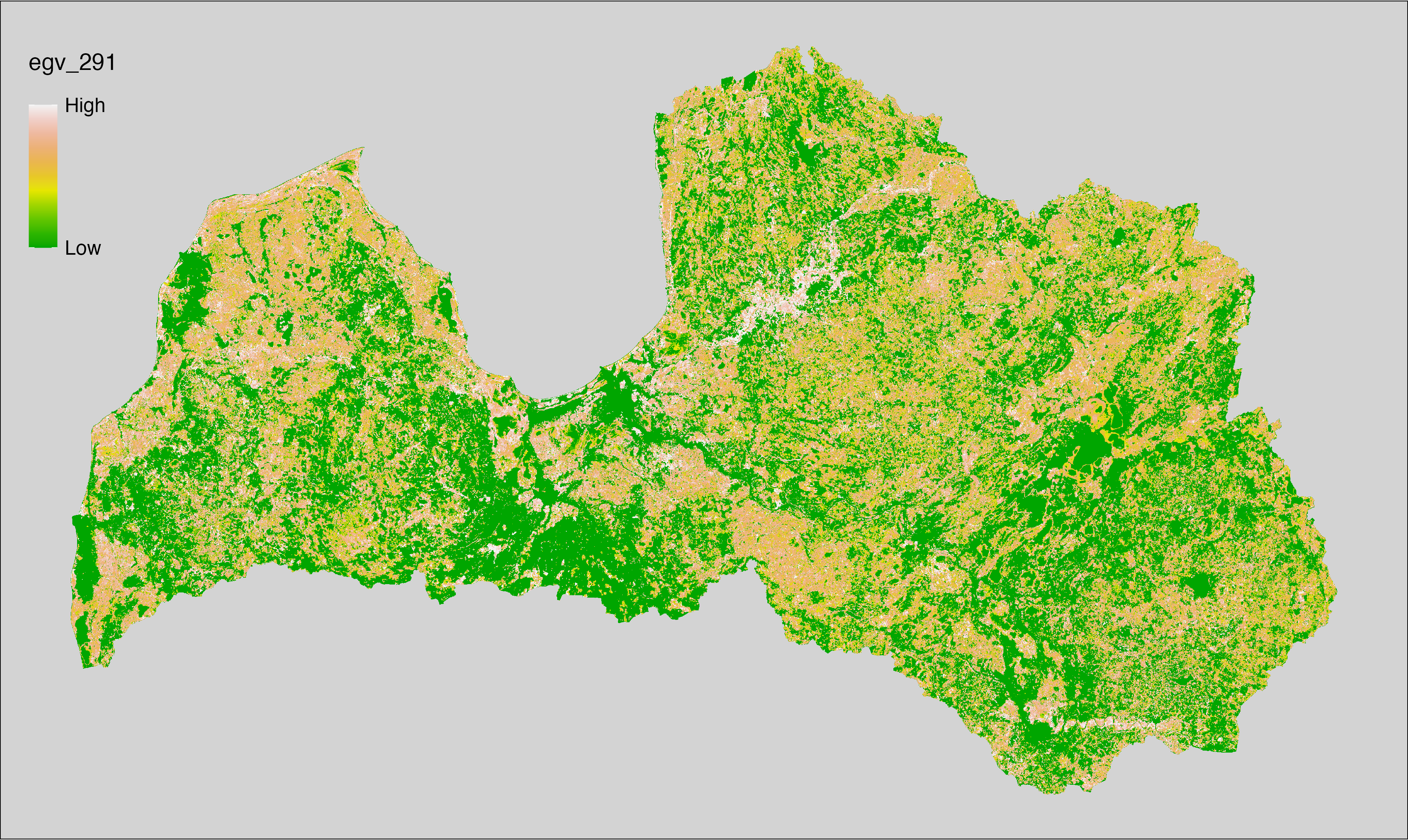
6.292 ForestsQuant_LargestDiameter-max_cell
filename: ForestsQuant_LargestDiameter-max_cell.tif
layername: egv_292
English name: Largest tree trunk diameter within the analysis cell (1 ha)
Latvian name: Lielākais koka stumbra diametrs analīzes šūnā (1 ha)
Procedure: Most EGVs describing forests are spatially restricted to areas outside of clearcuts and dead stands. This mask is created using a combination of the State Forest Service’s State Forest Registry land category 12 and 14, and The Global Forest Watch pixels classified as lost tree canopy cover since 2020 (raster layer matching input, presence = 1, absence = 0).
This EGV is prepared based on the information of the largest tree diameter per inventoried forest stand - State Forest Service’s State Forest Registry. This attribute has some extreme values. We chose to limit them to the nearest integer showing only minimal accumulation in histogram.
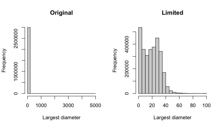
Resulting values at polygon geometries are rasterised with the workflow
egvtools::polygon2input(), restricting to pixels outside the clearcut mask. No
background values are assigned during rasterisation. The resulting layer is
then aggregated to EGV resolution using the workflow egvtools::input2egv() by calculating
maximum value. After the aggregation, cells with no forest information are
filled with value 0. Finally, the layer is standardised by subtracting
the arithmetic mean and dividing by the root mean squared error.
Code
# libs ----
if(!require(egvtools)) {remotes::install_github("aavotins/egvtools"); require(egvtools)}
if(!require(terra)) {install.packages("terra"); require(terra)}
if(!require(sf)) {install.packages("sf"); require(sf)}
if(!require(tidyverse)) {install.packages("tidyverse"); require(tidyverse)}
if(!require(sfarrow)) {install.packages("sfarrow"); require(sfarrow)}
if(!require(readxl)) {install.packages("readxl"); require(readxl)}
if(!require(raster)) {install.packages("raster"); require(raster)}
if(!require(fasterize)) {install.packages("fasterize"); require(fasterize)}
# templates ----
template100=rast("./Templates/TemplateRasters/LV100m_10km.tif")
template10=rast("./Templates/TemplateRasters/LV10m_10km.tif")
rastrs10=raster(template10)
nulls10=rast("./Templates/TemplateRasters/nulls_LV10m_10km.tif")
nulls100=rast("./Templates/TemplateRasters/nulls_LV100m_10km.tif")
# simple landscape ----
simple_landscape=rast("RasterGrids_10m/2024/Ainava_vienk_mask.tif")
# mvr ----
mvr=st_read_parquet("./Geodata/2024/MVR/nogabali_2024janv.parquet")
mvr$yes=1
# clear cut mask ----
izcirtumi=mvr %>%
filter(zkat %in% c("12","14")) %>%
dplyr::select(yes)
r_izcirtumi_mvr=fasterize(izcirtumi,rastrs10,field="yes")
t_izcirtumi_mvr=rast(r_izcirtumi_mvr)
plot(t_izcirtumi_mvr)
tcl=rast("./Geodata/2024/Trees/GFW/TreeCoverLoss_v1_12.tif")
tcl2=ifel(tcl<20,0,1)
tclX=cover(tcl2,nulls10)
plot(tclX)
clearcut_mask=cover(t_izcirtumi_mvr,tclX,
filename="./RasterGrids_10m/2024/Mask_clearcuts.tif",
overwrite=TRUE)
plot(clearcut_mask)
rm(izcirtumi)
rm(r_izcirtumi_mvr)
rm(t_izcirtumi_mvr)
rm(tcl)
rm(tcl2)
rm(tclX)
# ForestsQuant_LargestDiameter-max_cell.tif egv_292 ----
nogabali=mvr %>%
rowwise() %>%
mutate(maxDiam=max(c(d10,d11,d12,d13,d14,d22,d23,d24),na.rm=TRUE)) %>%
ungroup() %>%
mutate(maxDiam2=ifelse(maxDiam>100,100,maxDiam)) %>%
filter(!is.na(maxDiam2))
par(mfrow=c(1,2))
options(scipen=999)
hist(nogabali$maxDiam,main="Original",xlab="Largest diameter")
hist(nogabali$maxDiam2,main="Limited",xlab="Largest diameter")
par(mfrow=c(1,1))
options(scipen=0)
p2i_rez=polygon2input(vector_data=nogabali,
template_path = "./Templates/TemplateRasters/LV10m_10km.tif",
out_path = "./RasterGrids_10m/2024/",
file_name = "ForestsQuant_LargestDiameter.tif",
value_field = "maxDiam2",
fun="max",
prepare=FALSE,
restrict_to = clearcut_mask,
restrict_values = 0,
plot_result=TRUE,
overwrite=TRUE)
p2i_rez
i2e_rez=input2egv(input="./RasterGrids_10m/2024/ForestsQuant_LargestDiameter.tif",
egv_template = "./Templates/TemplateRasters/LV100m_10km.tif",
summary_function = "max",
missing_job = "CoverOutput",
output_bg = "./Templates/TemplateRasters/nulls_LV100m_10km.tif",
outlocation = "./RasterGrids_100m/2024/RAW/",
outfilename = "ForestsQuant_LargestDiameter-max_cell.tif",
layername = "egv_292",
plot_final=TRUE)
i2e_rez
rm(p2i_rez)
rm(nogabali)
rm(i2e_rez)
unlink("./RasterGrids_10m/2024/ForestsQuant_LargestDiameter.tif")
# standardisation ----
if(!require(terra)) {install.packages("terra"); require(terra)}
if(!require(tidyverse)) {install.packages("tidyverse"); require(tidyverse)}
nosaukums="ForestsQuant_LargestDiameter-max_cell.tif"
ielasisanas_cels=paste0("./RasterGrids_100m/2024/RAW/",nosaukums)
saglabasanas_cels=paste0("./RasterGrids_100m/2024/Scaled/",nosaukums)
slanis=rast(ielasisanas_cels)
videjais=global(slanis,fun="mean",na.rm=TRUE)
centrets=slanis-videjais[,1]
standartnovirze=terra::global(centrets,fun="rms",na.rm=TRUE)
merogots=centrets/standartnovirze[,1]
writeRaster(merogots,
filename=saglabasanas_cels,
overwrite=TRUE)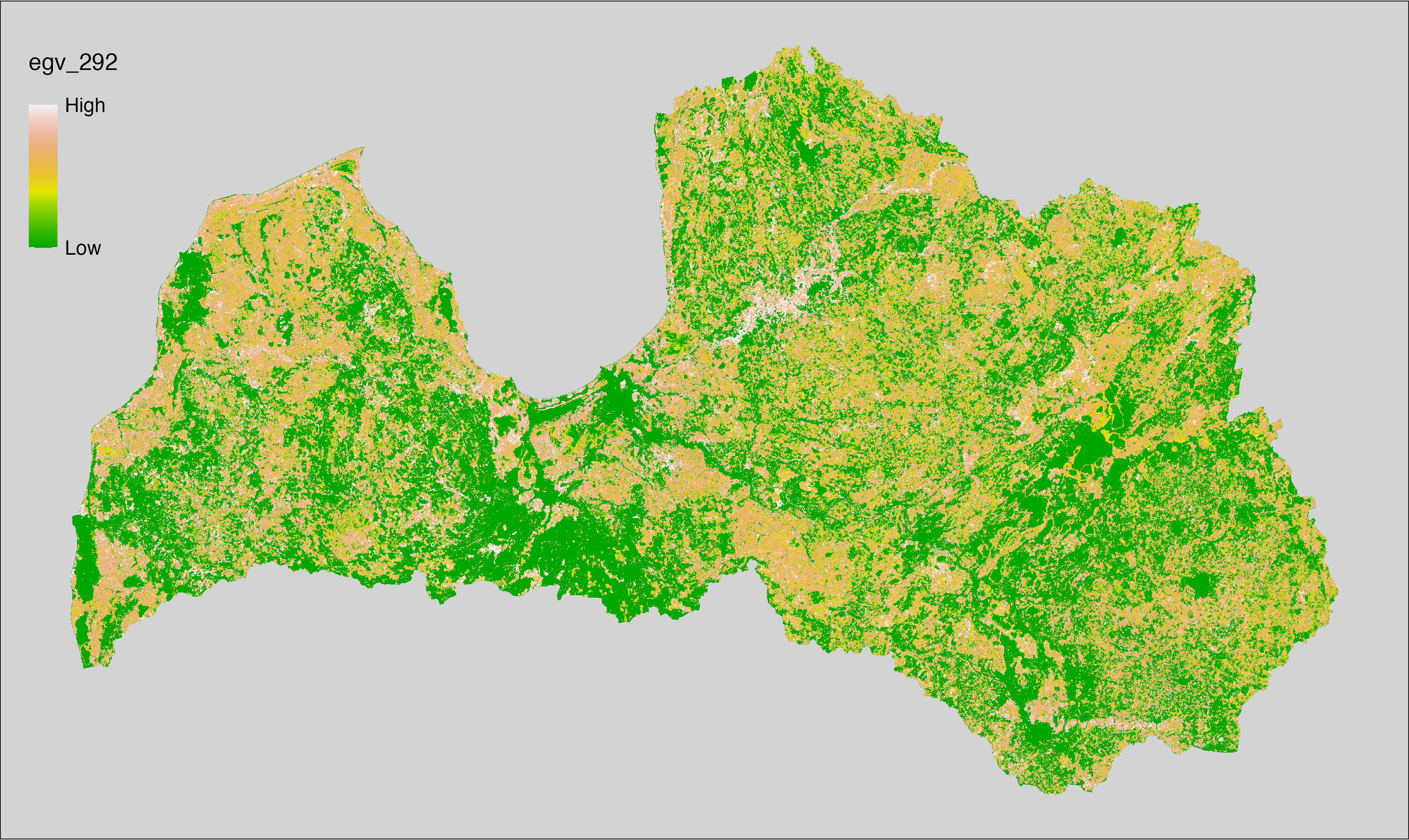
6.293 ForestsQuant_TimeSinceDisturbance-average_cell
filename: ForestsQuant_TimeSinceDisturbance-average_cell.tif
layername: egv_293
English name: Time since last disturbance affecting tree growing within the analysis cell (1 ha)
Latvian name: Laiks kopš pēdējā ar koku augšanu saistītā traucējuma analīzes šūnā (1 ha)
Procedure: This EGV is prepared primarily based on the information of the forestry related disturbances as registered per inventoried forest stand - State Forest Service’s State Forest Registry. The register, however, includes obvious errors - values later than 2024 and earlier than 1500 that are set to NA. Remaining values are subtracted from 2024. In stands with no disturbance registered, the age of dominant tree group is used to calculate minimum difference (age of time since disturbance) from the year 2024. This attribute has some extreme values. We chose to limit them to the nearest integer showing only minimal accumulation in histogram.
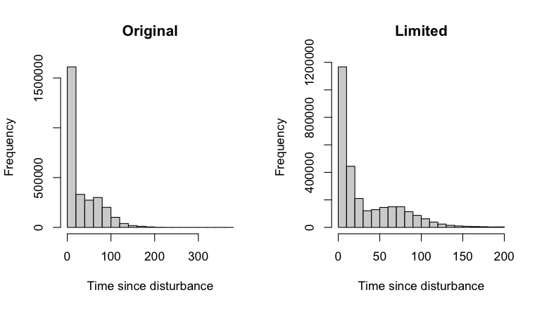
Resulting values at polygon geometries are rasterised (presence only). This
raster layer is then overlaid with reclassified year of tree cover loss
(reclassified to difference from the year 2024) and per pixel minimum value is
retained. As not all the forests or tree covered areas are inventoried, classes
from the Landscape classification are used to impute assumption of time
since tree growing disturbance - for class 620 we assume five years, whereas
for classes 630 and 640 - 50 years and 0 otherwise. Per pixel minimum layer is
then overlaid the assumed time since disturbance layer. The resulting layer is
then aggregated to EGV resolution using the workflow egvtools::input2egv() by calculating
arithmetic mean value. After the aggregation, inverse distance weighted (power =
2) gap filling is applied to avoid possible gaps at the edges. Finally, the layer
is standardised by subtracting the arithmetic mean and dividing by the root
mean squared error.
Code
# libs ----
if(!require(egvtools)) {remotes::install_github("aavotins/egvtools"); require(egvtools)}
if(!require(terra)) {install.packages("terra"); require(terra)}
if(!require(sf)) {install.packages("sf"); require(sf)}
if(!require(tidyverse)) {install.packages("tidyverse"); require(tidyverse)}
if(!require(sfarrow)) {install.packages("sfarrow"); require(sfarrow)}
if(!require(readxl)) {install.packages("readxl"); require(readxl)}
if(!require(raster)) {install.packages("raster"); require(raster)}
if(!require(fasterize)) {install.packages("fasterize"); require(fasterize)}
# templates ----
template100=rast("./Templates/TemplateRasters/LV100m_10km.tif")
template10=rast("./Templates/TemplateRasters/LV10m_10km.tif")
rastrs10=raster(template10)
nulls10=rast("./Templates/TemplateRasters/nulls_LV10m_10km.tif")
nulls100=rast("./Templates/TemplateRasters/nulls_LV100m_10km.tif")
# simple landscape ----
simple_landscape=rast("RasterGrids_10m/2024/Ainava_vienk_mask.tif")
# mvr ----
mvr=st_read_parquet("./Geodata/2024/MVR/nogabali_2024janv.parquet")
mvr$yes=1
# clear cut mask ----
izcirtumi=mvr %>%
filter(zkat %in% c("12","14")) %>%
dplyr::select(yes)
r_izcirtumi_mvr=fasterize(izcirtumi,rastrs10,field="yes")
t_izcirtumi_mvr=rast(r_izcirtumi_mvr)
plot(t_izcirtumi_mvr)
tcl=rast("./Geodata/2024/Trees/GFW/TreeCoverLoss_v1_12.tif")
tcl2=ifel(tcl<20,0,1)
tclX=cover(tcl2,nulls10)
plot(tclX)
clearcut_mask=cover(t_izcirtumi_mvr,tclX,
filename="./RasterGrids_10m/2024/Mask_clearcuts.tif",
overwrite=TRUE)
plot(clearcut_mask)
rm(izcirtumi)
rm(r_izcirtumi_mvr)
rm(t_izcirtumi_mvr)
rm(tcl)
rm(tcl2)
rm(tclX)
# ForestsQuant_TimeSinceDisturbance-average_cell.tif egv_293 ----
nogabali=mvr %>%
mutate(new_PDG=ifelse(p_darbg>2024,NA,
ifelse(p_darbv %in% c("1","4","5","6","7","10","11"),p_darbg,NA)),
new_PDG2=ifelse(new_PDG<1500,NA,new_PDG),
new_PCG=ifelse(p_cirg>2024,NA,p_cirg),
new_PCG2=ifelse(new_PCG<1500,NA,new_PCG),
vecumam=ifelse(a10==0,NA,a10),
new_PCG3=2024-new_PCG2,
new_PDG3=2024-new_PDG2) %>%
rowwise() %>%
mutate(Laikam=min(c(vecumam,new_PDG3,new_PCG3),na.rm=TRUE)) %>%
ungroup() %>%
mutate(KopsTraucejuma=ifelse(is.infinite(Laikam),NA,Laikam)) %>%
mutate(KopsTraucejuma2=ifelse(KopsTraucejuma>200,200,KopsTraucejuma)) %>%
filter(!is.na(KopsTraucejuma2))
par(mfrow=c(1,2))
options(scipen=999)
hist(nogabali$KopsTraucejuma,main="Original",xlab="Time since disturbance")
hist(nogabali$KopsTraucejuma2,main="Limited",xlab="Time since disturbance")
par(mfrow=c(1,1))
options(scipen=0)
mvr_trauclaiks=fasterize::fasterize(nogabali,rastrs10,field="KopsTraucejuma2",fun = "min")
t_MVRtrauclaiks=rast(mvr_trauclaiks)
plot(t_MVRtrauclaiks)
gfw=rast("./Geodata/2024/Trees/GFW/TreeCoverLoss_v1_12.tif")
plot(gfw)
gfw2=ifel(gfw>=0,24-gfw,NA)
plot(gfw2)
# No ainavas:
## Mežaudzes un koki = 50
## Krūmāji un parki = 5
## pārējais = 0
aizpildisanai=ifel(simple_landscape==630|simple_landscape==640,50,
ifel(simple_landscape==620,5,0))
freq(aizpildisanai)
trauclaiks1=terra::app(c(gfw2,t_MVRtrauclaiks),fun="min",na.rm=TRUE)
plot(trauclaiks1)
trauclaiks2=cover(trauclaiks1,aizpildisanai)
plot(trauclaiks2)
i2e_rez=input2egv(input=trauclaiks2,
egv_template = "./Templates/TemplateRasters/LV100m_10km.tif",
summary_function = "average",
missing_job = "FillOutput",
idw_weight = 2,
outlocation = "./RasterGrids_100m/2024/RAW/",
outfilename = "ForestsQuant_TimeSinceDisturbance-average_cell.tif",
layername = "egv_293",
plot_final=TRUE)
i2e_rez
rm(nogabali)
rm(mvr_trauclaiks)
rm(t_MVRtrauclaiks)
rm(gfw)
rm(gfw2)
rm(aizpildisanai)
rm(trauclaiks1)
rm(trauclaiks2)
rm(i2e_rez)
# standardisation ----
if(!require(terra)) {install.packages("terra"); require(terra)}
if(!require(tidyverse)) {install.packages("tidyverse"); require(tidyverse)}
nosaukums="ForestsQuant_TimeSinceDisturbance-average_cell.tif"
ielasisanas_cels=paste0("./RasterGrids_100m/2024/RAW/",nosaukums)
saglabasanas_cels=paste0("./RasterGrids_100m/2024/Scaled/",nosaukums)
slanis=rast(ielasisanas_cels)
videjais=global(slanis,fun="mean",na.rm=TRUE)
centrets=slanis-videjais[,1]
standartnovirze=terra::global(centrets,fun="rms",na.rm=TRUE)
merogots=centrets/standartnovirze[,1]
writeRaster(merogots,
filename=saglabasanas_cels,
overwrite=TRUE)
6.294 ForestsQuant_VolumeAspen-sum_cell
filename: ForestsQuant_VolumeAspen-sum_cell.tif
layername: egv_294
English name: Timber volume of Aspens, Poplars within the analysis cell (1 ha)
Latvian name: Apšu, papeļu krāja analīzes šūnā (1 ha)
Procedure: Most EGVs describing forests are spatially restricted to areas outside of clearcuts and dead stands. This mask is created using a combination of the State Forest Service’s State Forest Registry land category 12 and 14, and The Global Forest Watch pixels classified as lost tree canopy cover since 2020 (raster layer matching input, presence = 1, absence = 0).
This EGV is prepared based on the information of timber volume of aspen (species codes: 8, 19, 68; see tree species codes in Terminology and acronyms) in the inventoried forest stands - State Forest Service’s State Forest Registry. This attribute has some extreme values. We chose to limit them to the nearest integer showing only minimal accumulation in histogram.
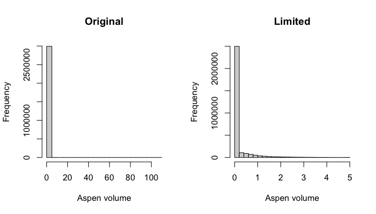
Resulting values at polygon geometries are rasterised with the workflow
egvtools::polygon2input(), restricting to pixels outside the clearcut mask. No
background values are assigned during rasterisation. The resulting layer is
then aggregated to EGV resolution using the workflow egvtools::input2egv() by calculating
sum of pixel values. After the aggregation, cells with no forest information
are filled with value 0. Finally, the layer is standardised by subtracting
the arithmetic mean and dividing by the root mean squared error.
Code
# libs ----
if(!require(egvtools)) {remotes::install_github("aavotins/egvtools"); require(egvtools)}
if(!require(terra)) {install.packages("terra"); require(terra)}
if(!require(sf)) {install.packages("sf"); require(sf)}
if(!require(tidyverse)) {install.packages("tidyverse"); require(tidyverse)}
if(!require(sfarrow)) {install.packages("sfarrow"); require(sfarrow)}
if(!require(readxl)) {install.packages("readxl"); require(readxl)}
if(!require(raster)) {install.packages("raster"); require(raster)}
if(!require(fasterize)) {install.packages("fasterize"); require(fasterize)}
# templates ----
template100=rast("./Templates/TemplateRasters/LV100m_10km.tif")
template10=rast("./Templates/TemplateRasters/LV10m_10km.tif")
rastrs10=raster(template10)
nulls10=rast("./Templates/TemplateRasters/nulls_LV10m_10km.tif")
nulls100=rast("./Templates/TemplateRasters/nulls_LV100m_10km.tif")
# simple landscape ----
simple_landscape=rast("RasterGrids_10m/2024/Ainava_vienk_mask.tif")
# mvr ----
mvr=st_read_parquet("./Geodata/2024/MVR/nogabali_2024janv.parquet")
mvr$yes=1
# clear cut mask ----
izcirtumi=mvr %>%
filter(zkat %in% c("12","14")) %>%
dplyr::select(yes)
r_izcirtumi_mvr=fasterize(izcirtumi,rastrs10,field="yes")
t_izcirtumi_mvr=rast(r_izcirtumi_mvr)
plot(t_izcirtumi_mvr)
tcl=rast("./Geodata/2024/Trees/GFW/TreeCoverLoss_v1_12.tif")
tcl2=ifel(tcl<20,0,1)
tclX=cover(tcl2,nulls10)
plot(tclX)
clearcut_mask=cover(t_izcirtumi_mvr,tclX,
filename="./RasterGrids_10m/2024/Mask_clearcuts.tif",
overwrite=TRUE)
plot(clearcut_mask)
rm(izcirtumi)
rm(r_izcirtumi_mvr)
rm(t_izcirtumi_mvr)
rm(tcl)
rm(tcl2)
rm(tclX)
# ForestsQuant_VolumeAspen-sum_cell.tif egv_294 ----
apses=c("8","19","68")
nogabali=mvr %>%
mutate(ApsuKraja=ifelse(s10 %in% apses, v10, 0)+ifelse(s11 %in% apses,v11,0)+
ifelse(s12 %in% apses, v12,0)+ifelse(s13 %in% apses,v13,0)+
ifelse(s14 %in% apses, v14,0)) %>%
mutate(ApsuKraja2=ApsuKraja/10000*10*10) %>%
mutate(ApsuKraja3=ifelse(ApsuKraja2>5,5,ApsuKraja2)) %>%
filter(!is.na(ApsuKraja2))
par(mfrow=c(1,2))
options(scipen=999)
hist(nogabali$ApsuKraja2,main="Original",xlab="Aspen volume")
hist(nogabali$ApsuKraja3,main="Limited",xlab="Aspen volume")
par(mfrow=c(1,1))
options(scipen=0)
p2i_rez=polygon2input(vector_data=nogabali,
template_path = "./Templates/TemplateRasters/LV10m_10km.tif",
out_path = "./RasterGrids_10m/2024/",
file_name = "ForestsQuant_VolumeAspen.tif",
value_field = "ApsuKraja3",
fun="max",
prepare=FALSE,
restrict_to = clearcut_mask,
restrict_values = 0,
plot_result=TRUE,
overwrite=TRUE)
p2i_rez
i2e_rez=input2egv(input="./RasterGrids_10m/2024/ForestsQuant_VolumeAspen.tif",
egv_template = "./Templates/TemplateRasters/LV100m_10km.tif",
summary_function = "sum",
missing_job = "CoverOutput",
output_bg = "./Templates/TemplateRasters/nulls_LV100m_10km.tif",
outlocation = "./RasterGrids_100m/2024/RAW/",
outfilename = "ForestsQuant_VolumeAspen-sum_cell.tif",
layername = "egv_294",
plot_final=TRUE)
i2e_rez
rm(p2i_rez)
rm(nogabali)
rm(apses)
rm(i2e_rez)
unlink("./RasterGrids_10m/2024/ForestsQuant_VolumeAspen.tif")
# standardisation ----
if(!require(terra)) {install.packages("terra"); require(terra)}
if(!require(tidyverse)) {install.packages("tidyverse"); require(tidyverse)}
nosaukums="ForestsQuant_VolumeAspen-sum_cell.tif"
ielasisanas_cels=paste0("./RasterGrids_100m/2024/RAW/",nosaukums)
saglabasanas_cels=paste0("./RasterGrids_100m/2024/Scaled/",nosaukums)
slanis=rast(ielasisanas_cels)
videjais=global(slanis,fun="mean",na.rm=TRUE)
centrets=slanis-videjais[,1]
standartnovirze=terra::global(centrets,fun="rms",na.rm=TRUE)
merogots=centrets/standartnovirze[,1]
writeRaster(merogots,
filename=saglabasanas_cels,
overwrite=TRUE)
6.295 ForestsQuant_VolumeBirch-sum_cell
filename: ForestsQuant_VolumeBirch-sum_cell.tif
layername: egv_295
English name: Timber volume of Birches within the analysis cell (1 ha)
Latvian name: Bērzu krāja analīzes šūnā (1 ha)
Procedure: Most EGVs describing forests are spatially restricted to areas outside of clearcuts and dead stands. This mask is created using a combination of the State Forest Service’s State Forest Registry land category 12 and 14, and The Global Forest Watch pixels classified as lost tree canopy cover since 2020 (raster layer matching input, presence = 1, absence = 0).
This EGV is prepared based on the information of timber volume of birch (species code: 4; see tree species codes in Terminology and acronyms) in the inventoried forest stands - State Forest Service’s State Forest Registry. This attribute has some extreme values. We chose to limit them to the nearest integer showing only minimal accumulation in histogram.
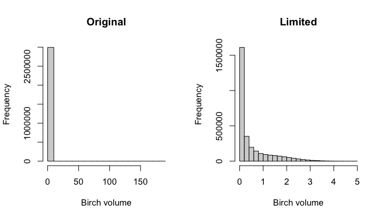
Resulting values at polygon geometries are rasterised with the workflow
egvtools::polygon2input(), restricting to pixels outside the clearcut mask. No
background values are assigned during rasterisation. The resulting layer is
then aggregated to EGV resolution using the workflow egvtools::input2egv() by calculating
sum of pixel values. After the aggregation, cells with no forest information
are filled with value 0. Finally, the layer is standardised by subtracting
the arithmetic mean and dividing by the root mean squared error.
Code
# libs ----
if(!require(egvtools)) {remotes::install_github("aavotins/egvtools"); require(egvtools)}
if(!require(terra)) {install.packages("terra"); require(terra)}
if(!require(sf)) {install.packages("sf"); require(sf)}
if(!require(tidyverse)) {install.packages("tidyverse"); require(tidyverse)}
if(!require(sfarrow)) {install.packages("sfarrow"); require(sfarrow)}
if(!require(readxl)) {install.packages("readxl"); require(readxl)}
if(!require(raster)) {install.packages("raster"); require(raster)}
if(!require(fasterize)) {install.packages("fasterize"); require(fasterize)}
# templates ----
template100=rast("./Templates/TemplateRasters/LV100m_10km.tif")
template10=rast("./Templates/TemplateRasters/LV10m_10km.tif")
rastrs10=raster(template10)
nulls10=rast("./Templates/TemplateRasters/nulls_LV10m_10km.tif")
nulls100=rast("./Templates/TemplateRasters/nulls_LV100m_10km.tif")
# simple landscape ----
simple_landscape=rast("RasterGrids_10m/2024/Ainava_vienk_mask.tif")
# mvr ----
mvr=st_read_parquet("./Geodata/2024/MVR/nogabali_2024janv.parquet")
mvr$yes=1
# clear cut mask ----
izcirtumi=mvr %>%
filter(zkat %in% c("12","14")) %>%
dplyr::select(yes)
r_izcirtumi_mvr=fasterize(izcirtumi,rastrs10,field="yes")
t_izcirtumi_mvr=rast(r_izcirtumi_mvr)
plot(t_izcirtumi_mvr)
tcl=rast("./Geodata/2024/Trees/GFW/TreeCoverLoss_v1_12.tif")
tcl2=ifel(tcl<20,0,1)
tclX=cover(tcl2,nulls10)
plot(tclX)
clearcut_mask=cover(t_izcirtumi_mvr,tclX,
filename="./RasterGrids_10m/2024/Mask_clearcuts.tif",
overwrite=TRUE)
plot(clearcut_mask)
rm(izcirtumi)
rm(r_izcirtumi_mvr)
rm(t_izcirtumi_mvr)
rm(tcl)
rm(tcl2)
rm(tclX)
# ForestsQuant_VolumeBirch-sum_cell.tif egv_295 ----
berzi=c("4")
nogabali=mvr %>%
mutate(BerzuKraja=ifelse(s10 %in% berzi, v10, 0)+ifelse(s11 %in% berzi,v11,0)+
ifelse(s12 %in% berzi, v12,0)+ifelse(s13 %in% berzi,v13,0)+
ifelse(s14 %in% berzi, v14,0)) %>%
mutate(BerzuKraja2=BerzuKraja/10000*10*10) %>%
mutate(BerzuKraja3=ifelse(BerzuKraja2>5,5,BerzuKraja2)) %>%
filter(!is.na(BerzuKraja2))
par(mfrow=c(1,2))
options(scipen=999)
hist(nogabali$BerzuKraja2,main="Original",xlab="Birch volume")
hist(nogabali$BerzuKraja3,main="Limited",xlab="Birch volume")
par(mfrow=c(1,1))
options(scipen=0)
p2i_rez=polygon2input(vector_data=nogabali,
template_path = "./Templates/TemplateRasters/LV10m_10km.tif",
out_path = "./RasterGrids_10m/2024/",
file_name = "ForestsQuant_VolumeBirch.tif",
value_field = "BerzuKraja3",
fun="max",
prepare=FALSE,
restrict_to = clearcut_mask,
restrict_values = 0,
plot_result=TRUE,
overwrite=TRUE)
p2i_rez
i2e_rez=input2egv(input="./RasterGrids_10m/2024/ForestsQuant_VolumeBirch.tif",
egv_template = "./Templates/TemplateRasters/LV100m_10km.tif",
summary_function = "sum",
missing_job = "CoverOutput",
output_bg = "./Templates/TemplateRasters/nulls_LV100m_10km.tif",
outlocation = "./RasterGrids_100m/2024/RAW/",
outfilename = "ForestsQuant_VolumeBirch-sum_cell.tif",
layername = "egv_295",
plot_final=TRUE)
i2e_rez
rm(p2i_rez)
rm(nogabali)
rm(berzi)
rm(i2e_rez)
unlink("./RasterGrids_10m/2024/ForestsQuant_VolumeBirch.tif")
# standardisation ----
if(!require(terra)) {install.packages("terra"); require(terra)}
if(!require(tidyverse)) {install.packages("tidyverse"); require(tidyverse)}
nosaukums="ForestsQuant_VolumeBirch-sum_cell.tif"
ielasisanas_cels=paste0("./RasterGrids_100m/2024/RAW/",nosaukums)
saglabasanas_cels=paste0("./RasterGrids_100m/2024/Scaled/",nosaukums)
slanis=rast(ielasisanas_cels)
videjais=global(slanis,fun="mean",na.rm=TRUE)
centrets=slanis-videjais[,1]
standartnovirze=terra::global(centrets,fun="rms",na.rm=TRUE)
merogots=centrets/standartnovirze[,1]
writeRaster(merogots,
filename=saglabasanas_cels,
overwrite=TRUE)
6.296 ForestsQuant_VolumeBlackAlder-sum_cell
filename: ForestsQuant_VolumeBlackAlder-sum_cell.tif
layername: egv_296
English name: Timber volume of Black Alder within the analysis cell (1 ha)
Latvian name: Melnalkšņu krāja analīzes šūnā (1 ha)
Procedure: Most EGVs describing forests are spatially restricted to areas outside of clearcuts and dead stands. This mask is created using a combination of the State Forest Service’s State Forest Registry land category 12 and 14, and The Global Forest Watch pixels classified as lost tree canopy cover since 2020 (raster layer matching input, presence = 1, absence = 0).
This EGV is prepared based on the information of timber volume of black alder (species code: 6; see tree species codes in Terminology and acronyms) in the inventoried forest stands - State Forest Service’s State Forest Registry. This attribute has some extreme values. We chose to limit them to the nearest integer showing only minimal accumulation in histogram.
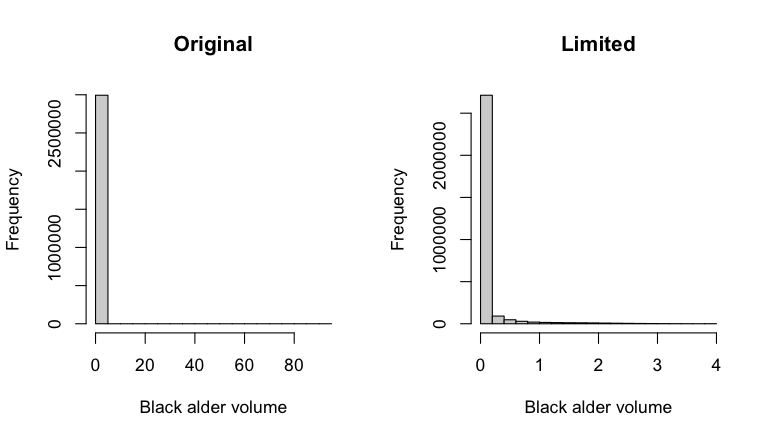
Resulting values at polygon geometries are rasterised with the workflow
egvtools::polygon2input(), restricting to pixels outside the clearcut mask. No
background values are assigned during rasterisation. The resulting layer is
then aggregated to EGV resolution using the workflow egvtools::input2egv() by calculating
sum of pixel values. After the aggregation, cells with no forest information
are filled with value 0. Finally, the layer is standardised by subtracting
the arithmetic mean and dividing by the root mean squared error.
Code
# libs ----
if(!require(egvtools)) {remotes::install_github("aavotins/egvtools"); require(egvtools)}
if(!require(terra)) {install.packages("terra"); require(terra)}
if(!require(sf)) {install.packages("sf"); require(sf)}
if(!require(tidyverse)) {install.packages("tidyverse"); require(tidyverse)}
if(!require(sfarrow)) {install.packages("sfarrow"); require(sfarrow)}
if(!require(readxl)) {install.packages("readxl"); require(readxl)}
if(!require(raster)) {install.packages("raster"); require(raster)}
if(!require(fasterize)) {install.packages("fasterize"); require(fasterize)}
# templates ----
template100=rast("./Templates/TemplateRasters/LV100m_10km.tif")
template10=rast("./Templates/TemplateRasters/LV10m_10km.tif")
rastrs10=raster(template10)
nulls10=rast("./Templates/TemplateRasters/nulls_LV10m_10km.tif")
nulls100=rast("./Templates/TemplateRasters/nulls_LV100m_10km.tif")
# simple landscape ----
simple_landscape=rast("RasterGrids_10m/2024/Ainava_vienk_mask.tif")
# mvr ----
mvr=st_read_parquet("./Geodata/2024/MVR/nogabali_2024janv.parquet")
mvr$yes=1
# clear cut mask ----
izcirtumi=mvr %>%
filter(zkat %in% c("12","14")) %>%
dplyr::select(yes)
r_izcirtumi_mvr=fasterize(izcirtumi,rastrs10,field="yes")
t_izcirtumi_mvr=rast(r_izcirtumi_mvr)
plot(t_izcirtumi_mvr)
tcl=rast("./Geodata/2024/Trees/GFW/TreeCoverLoss_v1_12.tif")
tcl2=ifel(tcl<20,0,1)
tclX=cover(tcl2,nulls10)
plot(tclX)
clearcut_mask=cover(t_izcirtumi_mvr,tclX,
filename="./RasterGrids_10m/2024/Mask_clearcuts.tif",
overwrite=TRUE)
plot(clearcut_mask)
rm(izcirtumi)
rm(r_izcirtumi_mvr)
rm(t_izcirtumi_mvr)
rm(tcl)
rm(tcl2)
rm(tclX)
# ForestsQuant_VolumeBlackAlder-sum_cell.tif egv_296 ----
melnalksni=c("6")
nogabali=mvr %>%
mutate(MeKraja=ifelse(s10 %in% melnalksni, v10, 0)+ifelse(s11 %in% melnalksni,v11,0)+
ifelse(s12 %in% melnalksni, v12,0)+ifelse(s13 %in% melnalksni,v13,0)+
ifelse(s14 %in% melnalksni, v14,0)) %>%
mutate(MeKraja2=MeKraja/10000*10*10) %>%
mutate(MeKraja3=ifelse(MeKraja2>4,4,MeKraja2)) %>%
filter(!is.na(MeKraja2))
par(mfrow=c(1,2))
options(scipen=999)
hist(nogabali$MeKraja2,main="Original",xlab="Black alder volume")
hist(nogabali$MeKraja3,main="Limited",xlab="Black alder volume")
par(mfrow=c(1,1))
options(scipen=0)
p2i_rez=polygon2input(vector_data=nogabali,
template_path = "./Templates/TemplateRasters/LV10m_10km.tif",
out_path = "./RasterGrids_10m/2024/",
file_name = "ForestsQuant_VolumeBlackAlder.tif",
value_field = "MeKraja3",
fun="max",
prepare=FALSE,
restrict_to = clearcut_mask,
restrict_values = 0,
plot_result=TRUE,
overwrite=TRUE)
p2i_rez
i2e_rez=input2egv(input="./RasterGrids_10m/2024/ForestsQuant_VolumeBlackAlder.tif",
egv_template = "./Templates/TemplateRasters/LV100m_10km.tif",
summary_function = "sum",
missing_job = "CoverOutput",
output_bg = "./Templates/TemplateRasters/nulls_LV100m_10km.tif",
outlocation = "./RasterGrids_100m/2024/RAW/",
outfilename = "ForestsQuant_VolumeBlackAlder-sum_cell.tif",
layername = "egv_296",
plot_final=TRUE)
i2e_rez
rm(p2i_rez)
rm(nogabali)
rm(melnalksni)
rm(i2e_rez)
unlink("./RasterGrids_10m/2024/ForestsQuant_VolumeBlackAlder.tif")
# standardisation ----
if(!require(terra)) {install.packages("terra"); require(terra)}
if(!require(tidyverse)) {install.packages("tidyverse"); require(tidyverse)}
nosaukums="ForestsQuant_VolumeBlackAlder-sum_cell.tif"
ielasisanas_cels=paste0("./RasterGrids_100m/2024/RAW/",nosaukums)
saglabasanas_cels=paste0("./RasterGrids_100m/2024/Scaled/",nosaukums)
slanis=rast(ielasisanas_cels)
videjais=global(slanis,fun="mean",na.rm=TRUE)
centrets=slanis-videjais[,1]
standartnovirze=terra::global(centrets,fun="rms",na.rm=TRUE)
merogots=centrets/standartnovirze[,1]
writeRaster(merogots,
filename=saglabasanas_cels,
overwrite=TRUE)
6.297 ForestsQuant_VolumeBorealDeciduousOther-sum_cell
filename: ForestsQuant_VolumeBorealDeciduousOther-sum_cell.tif
layername: egv_297
English name: Timber volume of Other Boreal Deciduous trees within the analysis cell (1 ha)
Latvian name: Citu šaurlapju krāja analīzes šūnā (1 ha)
Procedure: Most EGVs describing forests are spatially restricted to areas outside of clearcuts and dead stands. This mask is created using a combination of the State Forest Service’s State Forest Registry land category 12 and 14, and The Global Forest Watch pixels classified as lost tree canopy cover since 2020 (raster layer matching input, presence = 1, absence = 0).
This EGV is prepared based on the information of timber volume of Boreal deciduous tree species not separately described with own EGVs (species codes: 9, 20, 21, 32, 35; see tree species codes in Terminology and acronyms) in the inventoried forest stands - State Forest Service’s State Forest Registry. This attribute has some extreme values. We chose to limit them to the nearest integer showing only minimal accumulation in histogram.
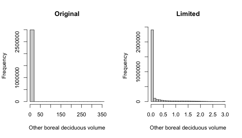
Resulting values at polygon geometries are rasterised with the workflow
egvtools::polygon2input(), restricting to pixels outside the clearcut mask. No
background values are assigned during rasterisation. The resulting layer is
then aggregated to EGV resolution using the workflow egvtools::input2egv() by calculating
sum of pixel values. After the aggregation, cells with no forest information
are filled with value 0. Finally, the layer is standardised by subtracting
the arithmetic mean and dividing by the root mean squared error.
Code
# libs ----
if(!require(egvtools)) {remotes::install_github("aavotins/egvtools"); require(egvtools)}
if(!require(terra)) {install.packages("terra"); require(terra)}
if(!require(sf)) {install.packages("sf"); require(sf)}
if(!require(tidyverse)) {install.packages("tidyverse"); require(tidyverse)}
if(!require(sfarrow)) {install.packages("sfarrow"); require(sfarrow)}
if(!require(readxl)) {install.packages("readxl"); require(readxl)}
if(!require(raster)) {install.packages("raster"); require(raster)}
if(!require(fasterize)) {install.packages("fasterize"); require(fasterize)}
# templates ----
template100=rast("./Templates/TemplateRasters/LV100m_10km.tif")
template10=rast("./Templates/TemplateRasters/LV10m_10km.tif")
rastrs10=raster(template10)
nulls10=rast("./Templates/TemplateRasters/nulls_LV10m_10km.tif")
nulls100=rast("./Templates/TemplateRasters/nulls_LV100m_10km.tif")
# simple landscape ----
simple_landscape=rast("RasterGrids_10m/2024/Ainava_vienk_mask.tif")
# mvr ----
mvr=st_read_parquet("./Geodata/2024/MVR/nogabali_2024janv.parquet")
mvr$yes=1
# clear cut mask ----
izcirtumi=mvr %>%
filter(zkat %in% c("12","14")) %>%
dplyr::select(yes)
r_izcirtumi_mvr=fasterize(izcirtumi,rastrs10,field="yes")
t_izcirtumi_mvr=rast(r_izcirtumi_mvr)
plot(t_izcirtumi_mvr)
tcl=rast("./Geodata/2024/Trees/GFW/TreeCoverLoss_v1_12.tif")
tcl2=ifel(tcl<20,0,1)
tclX=cover(tcl2,nulls10)
plot(tclX)
clearcut_mask=cover(t_izcirtumi_mvr,tclX,
filename="./RasterGrids_10m/2024/Mask_clearcuts.tif",
overwrite=TRUE)
plot(clearcut_mask)
rm(izcirtumi)
rm(r_izcirtumi_mvr)
rm(t_izcirtumi_mvr)
rm(tcl)
rm(tcl2)
rm(tclX)
# ForestsQuant_VolumeBorealDeciduousOther-sum_cell.tif egv_297 ----
sl_citi=c("9","20","21","32","35")
nogabali=mvr %>%
mutate(SaurlapjuCKraja=ifelse(s10 %in% sl_citi, v10, 0)+ifelse(s11 %in% sl_citi,v11,0)+
ifelse(s12 %in% sl_citi, v12,0)+ifelse(s13 %in% sl_citi,v13,0)+
ifelse(s14 %in% sl_citi, v14,0)) %>%
mutate(SaurlapjuCKraja2=SaurlapjuCKraja/10000*10*10) %>%
mutate(SaurlapjuCKraja3=ifelse(SaurlapjuCKraja2>3,3,SaurlapjuCKraja2)) %>%
filter(!is.na(SaurlapjuCKraja2))
par(mfrow=c(1,2))
options(scipen=999)
hist(nogabali$SaurlapjuCKraja2,main="Original",xlab="Other Boreal deciduous volume")
hist(nogabali$SaurlapjuCKraja3,main="Limited",xlab="Other Boreal deciduous volume")
par(mfrow=c(1,1))
options(scipen=0)
p2i_rez=polygon2input(vector_data=nogabali,
template_path = "./Templates/TemplateRasters/LV10m_10km.tif",
out_path = "./RasterGrids_10m/2024/",
file_name = "ForestsQuant_VolumeBorealDeciduousOther.tif",
value_field = "SaurlapjuCKraja3",
fun="max",
prepare=FALSE,
restrict_to = clearcut_mask,
restrict_values = 0,
plot_result=TRUE,
overwrite=TRUE)
p2i_rez
i2e_rez=input2egv(input="./RasterGrids_10m/2024/ForestsQuant_VolumeBorealDeciduousOther.tif",
egv_template = "./Templates/TemplateRasters/LV100m_10km.tif",
summary_function = "sum",
missing_job = "CoverOutput",
output_bg = "./Templates/TemplateRasters/nulls_LV100m_10km.tif",
outlocation = "./RasterGrids_100m/2024/RAW/",
outfilename = "ForestsQuant_VolumeBorealDeciduousOther-sum_cell.tif",
layername = "egv_297",
plot_final=TRUE)
i2e_rez
rm(p2i_rez)
rm(nogabali)
rm(sl_citi)
rm(i2e_rez)
unlink("./RasterGrids_10m/2024/ForestsQuant_VolumeBorealDeciduousOther.tif")
# standardisation ----
if(!require(terra)) {install.packages("terra"); require(terra)}
if(!require(tidyverse)) {install.packages("tidyverse"); require(tidyverse)}
nosaukums="ForestsQuant_VolumeBorealDeciduousOther-sum_cell.tif"
ielasisanas_cels=paste0("./RasterGrids_100m/2024/RAW/",nosaukums)
saglabasanas_cels=paste0("./RasterGrids_100m/2024/Scaled/",nosaukums)
slanis=rast(ielasisanas_cels)
videjais=global(slanis,fun="mean",na.rm=TRUE)
centrets=slanis-videjais[,1]
standartnovirze=terra::global(centrets,fun="rms",na.rm=TRUE)
merogots=centrets/standartnovirze[,1]
writeRaster(merogots,
filename=saglabasanas_cels,
overwrite=TRUE)
6.298 ForestsQuant_VolumeBorealDeciduousTotal-sum_cell
filename: ForestsQuant_VolumeBorealDeciduousTotal-sum_cell.tif
layername: egv_298
English name: Timber volume of Boreal Deciduous trees within the analysis cell (1 ha)
Latvian name: Šaurlapju krāja analīzes šūnā (1 ha)
Procedure: Most EGVs describing forests are spatially restricted to areas outside of clearcuts and dead stands. This mask is created using a combination of the State Forest Service’s State Forest Registry land category 12 and 14, and The Global Forest Watch pixels classified as lost tree canopy cover since 2020 (raster layer matching input, presence = 1, absence = 0).
This EGV is prepared based on the information of timber volume of Boreal deciduous tree species (species codes: 4, 6, 8, 9, 19, 20, 21, 32, 35, 68; see tree species codes in Terminology and acronyms) in the inventoried forest stands - State Forest Service’s State Forest Registry. This attribute has some extreme values. We chose to limit them to the nearest integer showing only minimal accumulation in histogram.
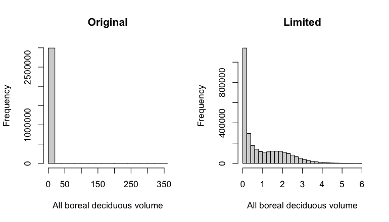
Resulting values at polygon geometries are rasterised with the workflow
egvtools::polygon2input(), restricting to pixels outside the clearcut mask. No
background values are assigned during rasterisation. The resulting layer is
then aggregated to EGV resolution using the workflow egvtools::input2egv() by calculating
sum of pixel values. After the aggregation, cells with no forest information
are filled with value 0. Finally, the layer is standardised by subtracting
the arithmetic mean and dividing by the root mean squared error.
Code
# libs ----
if(!require(egvtools)) {remotes::install_github("aavotins/egvtools"); require(egvtools)}
if(!require(terra)) {install.packages("terra"); require(terra)}
if(!require(sf)) {install.packages("sf"); require(sf)}
if(!require(tidyverse)) {install.packages("tidyverse"); require(tidyverse)}
if(!require(sfarrow)) {install.packages("sfarrow"); require(sfarrow)}
if(!require(readxl)) {install.packages("readxl"); require(readxl)}
if(!require(raster)) {install.packages("raster"); require(raster)}
if(!require(fasterize)) {install.packages("fasterize"); require(fasterize)}
# templates ----
template100=rast("./Templates/TemplateRasters/LV100m_10km.tif")
template10=rast("./Templates/TemplateRasters/LV10m_10km.tif")
rastrs10=raster(template10)
nulls10=rast("./Templates/TemplateRasters/nulls_LV10m_10km.tif")
nulls100=rast("./Templates/TemplateRasters/nulls_LV100m_10km.tif")
# simple landscape ----
simple_landscape=rast("RasterGrids_10m/2024/Ainava_vienk_mask.tif")
# mvr ----
mvr=st_read_parquet("./Geodata/2024/MVR/nogabali_2024janv.parquet")
mvr$yes=1
# clear cut mask ----
izcirtumi=mvr %>%
filter(zkat %in% c("12","14")) %>%
dplyr::select(yes)
r_izcirtumi_mvr=fasterize(izcirtumi,rastrs10,field="yes")
t_izcirtumi_mvr=rast(r_izcirtumi_mvr)
plot(t_izcirtumi_mvr)
tcl=rast("./Geodata/2024/Trees/GFW/TreeCoverLoss_v1_12.tif")
tcl2=ifel(tcl<20,0,1)
tclX=cover(tcl2,nulls10)
plot(tclX)
clearcut_mask=cover(t_izcirtumi_mvr,tclX,
filename="./RasterGrids_10m/2024/Mask_clearcuts.tif",
overwrite=TRUE)
plot(clearcut_mask)
rm(izcirtumi)
rm(r_izcirtumi_mvr)
rm(t_izcirtumi_mvr)
rm(tcl)
rm(tcl2)
rm(tclX)
# ForestsQuant_VolumeBorealDeciduousTotal-sum_cell.tif egv_298 ----
sl_visi=c("4","6","8","9","19","20","21","32","35","68")
nogabali=mvr %>%
mutate(SaurlapjuVKraja=ifelse(s10 %in% sl_visi, v10, 0)+ifelse(s11 %in% sl_visi,v11,0)+
ifelse(s12 %in% sl_visi, v12,0)+ifelse(s13 %in% sl_visi,v13,0)+
ifelse(s14 %in% sl_visi, v14,0)) %>%
mutate(SaurlapjuVKraja2=SaurlapjuVKraja/10000*10*10) %>%
mutate(SaurlapjuVKraja3=ifelse(SaurlapjuVKraja2>6,6,SaurlapjuVKraja2)) %>%
filter(!is.na(SaurlapjuVKraja2))
par(mfrow=c(1,2))
options(scipen=999)
hist(nogabali$SaurlapjuVKraja2,main="Original",xlab="All Boreal deciduous volume")
hist(nogabali$SaurlapjuVKraja3,main="Limited",xlab="All Boreal deciduous volume")
par(mfrow=c(1,1))
options(scipen=0)
p2i_rez=polygon2input(vector_data=nogabali,
template_path = "./Templates/TemplateRasters/LV10m_10km.tif",
out_path = "./RasterGrids_10m/2024/",
file_name = "ForestsQuant_VolumeBorealDeciduousTotal.tif",
value_field = "SaurlapjuVKraja3",
fun="max",
prepare=FALSE,
restrict_to = clearcut_mask,
restrict_values = 0,
plot_result=TRUE,
overwrite=TRUE)
p2i_rez
i2e_rez=input2egv(input="./RasterGrids_10m/2024/ForestsQuant_VolumeBorealDeciduousTotal.tif",
egv_template = "./Templates/TemplateRasters/LV100m_10km.tif",
summary_function = "sum",
missing_job = "CoverOutput",
output_bg = "./Templates/TemplateRasters/nulls_LV100m_10km.tif",
outlocation = "./RasterGrids_100m/2024/RAW/",
outfilename = "ForestsQuant_VolumeBorealDeciduousTotal-sum_cell.tif",
layername = "egv_298",
plot_final=TRUE)
i2e_rez
rm(p2i_rez)
rm(nogabali)
rm(sl_visi)
rm(i2e_rez)
unlink("./RasterGrids_10m/2024/ForestsQuant_VolumeBorealDeciduousTotal.tif")
# standardisation ----
if(!require(terra)) {install.packages("terra"); require(terra)}
if(!require(tidyverse)) {install.packages("tidyverse"); require(tidyverse)}
nosaukums="ForestsQuant_VolumeBorealDeciduousTotal-sum_cell.tif"
ielasisanas_cels=paste0("./RasterGrids_100m/2024/RAW/",nosaukums)
saglabasanas_cels=paste0("./RasterGrids_100m/2024/Scaled/",nosaukums)
slanis=rast(ielasisanas_cels)
videjais=global(slanis,fun="mean",na.rm=TRUE)
centrets=slanis-videjais[,1]
standartnovirze=terra::global(centrets,fun="rms",na.rm=TRUE)
merogots=centrets/standartnovirze[,1]
writeRaster(merogots,
filename=saglabasanas_cels,
overwrite=TRUE)
6.299 ForestsQuant_VolumeConiferous-sum_cell
filename: ForestsQuant_VolumeConiferous-sum_cell.tif
layername: egv_299
English name: Timber volume of Coniferous trees within the analysis cell (1 ha)
Latvian name: Skujkoku krāja analīzes šūnā (1 ha)
Procedure: Most EGVs describing forests are spatially restricted to areas outside of clearcuts and dead stands. This mask is created using a combination of the State Forest Service’s State Forest Registry land category 12 and 14, and The Global Forest Watch pixels classified as lost tree canopy cover since 2020 (raster layer matching input, presence = 1, absence = 0).
This EGV is prepared based on the information of timber volume of coniferous tree species (species codes: 1, 14, 22, 3, 13, 15, 23, 28; see tree species codes in Terminology and acronyms) in the inventoried forest stands - State Forest Service’s State Forest Registry. This attribute has some extreme values. We chose to limit them to the nearest integer showing only minimal accumulation in histogram.
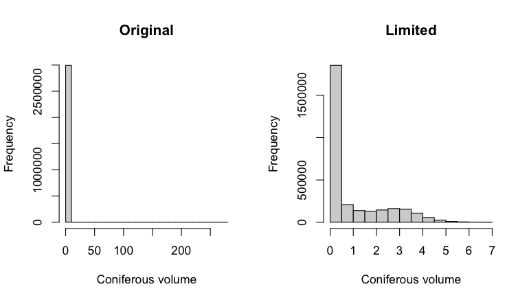
Resulting values at polygon geometries are rasterised with the workflow
egvtools::polygon2input(), restricting to pixels outside the clearcut mask. No
background values are assigned during rasterisation. The resulting layer is
then aggregated to EGV resolution using the workflow egvtools::input2egv() by calculating
sum of pixel values. After the aggregation, cells with no forest information
are filled with value 0. Finally, the layer is standardised by subtracting
the arithmetic mean and dividing by the root mean squared error.
Code
# libs ----
if(!require(egvtools)) {remotes::install_github("aavotins/egvtools"); require(egvtools)}
if(!require(terra)) {install.packages("terra"); require(terra)}
if(!require(sf)) {install.packages("sf"); require(sf)}
if(!require(tidyverse)) {install.packages("tidyverse"); require(tidyverse)}
if(!require(sfarrow)) {install.packages("sfarrow"); require(sfarrow)}
if(!require(readxl)) {install.packages("readxl"); require(readxl)}
if(!require(raster)) {install.packages("raster"); require(raster)}
if(!require(fasterize)) {install.packages("fasterize"); require(fasterize)}
# templates ----
template100=rast("./Templates/TemplateRasters/LV100m_10km.tif")
template10=rast("./Templates/TemplateRasters/LV10m_10km.tif")
rastrs10=raster(template10)
nulls10=rast("./Templates/TemplateRasters/nulls_LV10m_10km.tif")
nulls100=rast("./Templates/TemplateRasters/nulls_LV100m_10km.tif")
# simple landscape ----
simple_landscape=rast("RasterGrids_10m/2024/Ainava_vienk_mask.tif")
# mvr ----
mvr=st_read_parquet("./Geodata/2024/MVR/nogabali_2024janv.parquet")
mvr$yes=1
# clear cut mask ----
izcirtumi=mvr %>%
filter(zkat %in% c("12","14")) %>%
dplyr::select(yes)
r_izcirtumi_mvr=fasterize(izcirtumi,rastrs10,field="yes")
t_izcirtumi_mvr=rast(r_izcirtumi_mvr)
plot(t_izcirtumi_mvr)
tcl=rast("./Geodata/2024/Trees/GFW/TreeCoverLoss_v1_12.tif")
tcl2=ifel(tcl<20,0,1)
tclX=cover(tcl2,nulls10)
plot(tclX)
clearcut_mask=cover(t_izcirtumi_mvr,tclX,
filename="./RasterGrids_10m/2024/Mask_clearcuts.tif",
overwrite=TRUE)
plot(clearcut_mask)
rm(izcirtumi)
rm(r_izcirtumi_mvr)
rm(t_izcirtumi_mvr)
rm(tcl)
rm(tcl2)
rm(tclX)
# ForestsQuant_VolumeConiferous-sum_cell.tif egv_299 ----
skujkoki=c("1","14","22","3","13","15","23","28")
nogabali=mvr %>%
mutate(SkujkokuKraja=ifelse(s10 %in% skujkoki, v10, 0)+ifelse(s11 %in% skujkoki,v11,0)+
ifelse(s12 %in% skujkoki, v12,0)+ifelse(s13 %in% skujkoki,v13,0)+
ifelse(s14 %in% skujkoki, v14,0)) %>%
mutate(SkujkokuKraja2=SkujkokuKraja/10000*10*10) %>%
mutate(SkujkokuKraja3=ifelse(SkujkokuKraja2>7,7,SkujkokuKraja2)) %>%
filter(!is.na(SkujkokuKraja2))
par(mfrow=c(1,2))
options(scipen=999)
hist(nogabali$SkujkokuKraja2,main="Original",xlab="Coniferous volume")
hist(nogabali$SkujkokuKraja3,main="Limited",xlab="Coniferous volume")
par(mfrow=c(1,1))
options(scipen=0)
p2i_rez=polygon2input(vector_data=nogabali,
template_path = "./Templates/TemplateRasters/LV10m_10km.tif",
out_path = "./RasterGrids_10m/2024/",
file_name = "ForestsQuant_VolumeConiferous.tif",
value_field = "SkujkokuKraja3",
fun="max",
prepare=FALSE,
restrict_to = clearcut_mask,
restrict_values = 0,
plot_result=TRUE,
overwrite=TRUE)
p2i_rez
i2e_rez=input2egv(input="./RasterGrids_10m/2024/ForestsQuant_VolumeConiferous.tif",
egv_template = "./Templates/TemplateRasters/LV100m_10km.tif",
summary_function = "sum",
missing_job = "CoverOutput",
output_bg = "./Templates/TemplateRasters/nulls_LV100m_10km.tif",
outlocation = "./RasterGrids_100m/2024/RAW/",
outfilename = "ForestsQuant_VolumeConiferous-sum_cell.tif",
layername = "egv_299",
plot_final=TRUE)
i2e_rez
rm(p2i_rez)
rm(nogabali)
rm(skujkoki)
rm(i2e_rez)
unlink("./RasterGrids_10m/2024/ForestsQuant_VolumeConiferous.tif")
# standardisation ----
if(!require(terra)) {install.packages("terra"); require(terra)}
if(!require(tidyverse)) {install.packages("tidyverse"); require(tidyverse)}
nosaukums="ForestsQuant_VolumeConiferous-sum_cell.tif"
ielasisanas_cels=paste0("./RasterGrids_100m/2024/RAW/",nosaukums)
saglabasanas_cels=paste0("./RasterGrids_100m/2024/Scaled/",nosaukums)
slanis=rast(ielasisanas_cels)
videjais=global(slanis,fun="mean",na.rm=TRUE)
centrets=slanis-videjais[,1]
standartnovirze=terra::global(centrets,fun="rms",na.rm=TRUE)
merogots=centrets/standartnovirze[,1]
writeRaster(merogots,
filename=saglabasanas_cels,
overwrite=TRUE)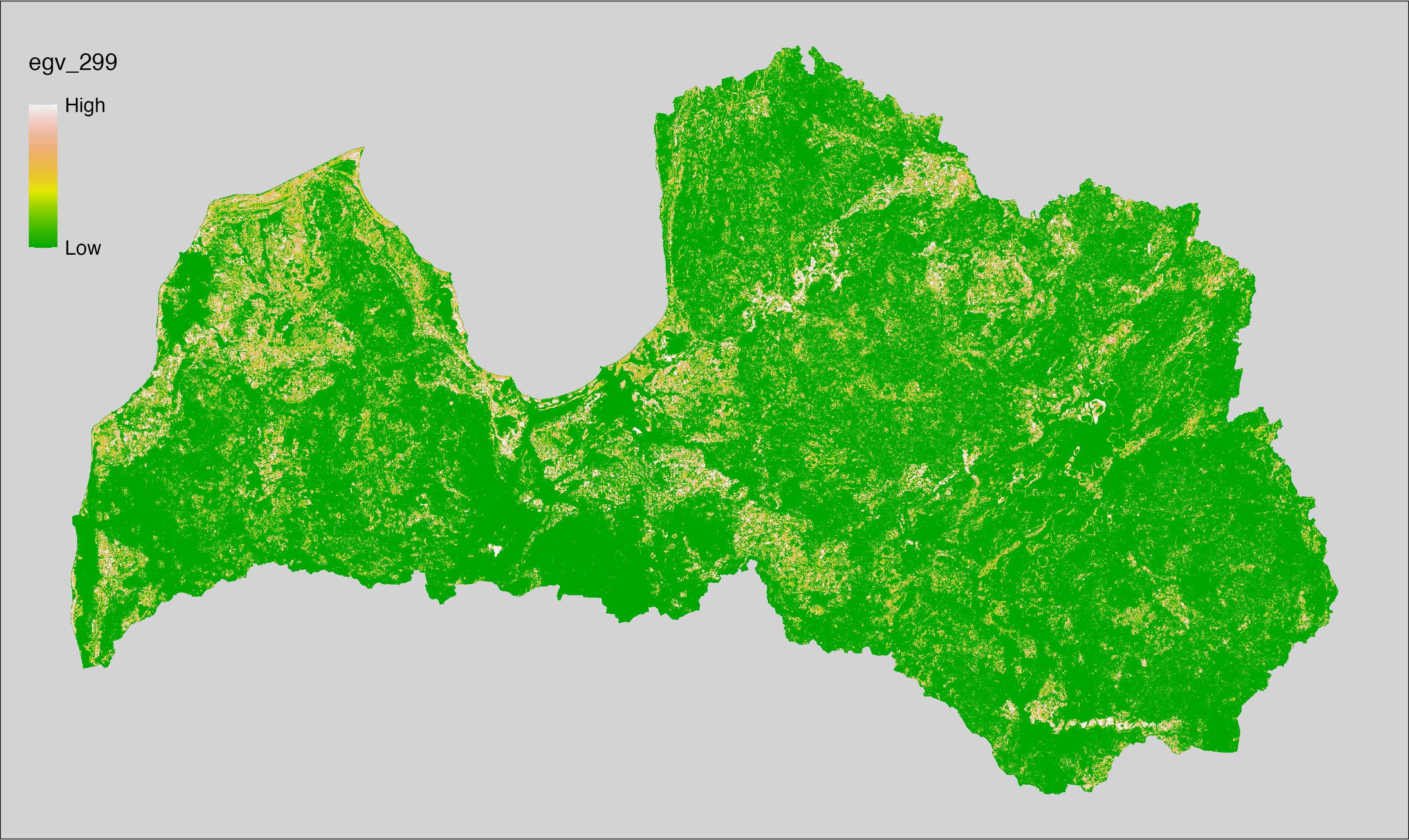
6.300 ForestsQuant_VolumeOak-sum_cell
filename: ForestsQuant_VolumeOak-sum_cell.tif
layername: egv_300
English name: Timber volume of Oaks within the analysis cell (1 ha)
Latvian name: Ozolu krāja analīzes šūnā (1 ha)
Procedure: Most EGVs describing forests are spatially restricted to areas outside of clearcuts and dead stands. This mask is created using a combination of the State Forest Service’s State Forest Registry land category 12 and 14, and The Global Forest Watch pixels classified as lost tree canopy cover since 2020 (raster layer matching input, presence = 1, absence = 0).
This EGV is prepared based on the information of timber volume of oaks (species codes: 10, 61; see tree species codes in Terminology and acronyms) in the inventoried forest stands - State Forest Service’s State Forest Registry. This attribute has some extreme values. We chose to limit them to the nearest integer showing only minimal accumulation in histogram.
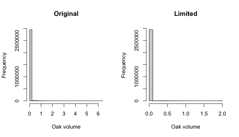
Resulting values at polygon geometries are rasterised with the workflow
egvtools::polygon2input(), restricting to pixels outside the clearcut mask. No
background values are assigned during rasterisation. The resulting layer is
then aggregated to EGV resolution using the workflow egvtools::input2egv() by calculating
sum of pixel values. After the aggregation, cells with no forest information
are filled with value 0. Finally, the layer is standardised by subtracting
the arithmetic mean and dividing by the root mean squared error.
Code
# libs ----
if(!require(egvtools)) {remotes::install_github("aavotins/egvtools"); require(egvtools)}
if(!require(terra)) {install.packages("terra"); require(terra)}
if(!require(sf)) {install.packages("sf"); require(sf)}
if(!require(tidyverse)) {install.packages("tidyverse"); require(tidyverse)}
if(!require(sfarrow)) {install.packages("sfarrow"); require(sfarrow)}
if(!require(readxl)) {install.packages("readxl"); require(readxl)}
if(!require(raster)) {install.packages("raster"); require(raster)}
if(!require(fasterize)) {install.packages("fasterize"); require(fasterize)}
# templates ----
template100=rast("./Templates/TemplateRasters/LV100m_10km.tif")
template10=rast("./Templates/TemplateRasters/LV10m_10km.tif")
rastrs10=raster(template10)
nulls10=rast("./Templates/TemplateRasters/nulls_LV10m_10km.tif")
nulls100=rast("./Templates/TemplateRasters/nulls_LV100m_10km.tif")
# simple landscape ----
simple_landscape=rast("RasterGrids_10m/2024/Ainava_vienk_mask.tif")
# mvr ----
mvr=st_read_parquet("./Geodata/2024/MVR/nogabali_2024janv.parquet")
mvr$yes=1
# clear cut mask ----
izcirtumi=mvr %>%
filter(zkat %in% c("12","14")) %>%
dplyr::select(yes)
r_izcirtumi_mvr=fasterize(izcirtumi,rastrs10,field="yes")
t_izcirtumi_mvr=rast(r_izcirtumi_mvr)
plot(t_izcirtumi_mvr)
tcl=rast("./Geodata/2024/Trees/GFW/TreeCoverLoss_v1_12.tif")
tcl2=ifel(tcl<20,0,1)
tclX=cover(tcl2,nulls10)
plot(tclX)
clearcut_mask=cover(t_izcirtumi_mvr,tclX,
filename="./RasterGrids_10m/2024/Mask_clearcuts.tif",
overwrite=TRUE)
plot(clearcut_mask)
rm(izcirtumi)
rm(r_izcirtumi_mvr)
rm(t_izcirtumi_mvr)
rm(tcl)
rm(tcl2)
rm(tclX)
# ForestsQuant_VolumeOak-sum_cell.tif egv_300 ----
ozoli=c("10","61")
nogabali=mvr %>%
mutate(OzoluKraja=ifelse(s10 %in% ozoli, v10, 0)+ifelse(s11 %in% ozoli,v11,0)+
ifelse(s12 %in% ozoli, v12,0)+ifelse(s13 %in% ozoli,v13,0)+
ifelse(s14 %in% ozoli, v14,0)) %>%
mutate(OzoluKraja2=OzoluKraja/10000*10*10) %>%
mutate(OzoluKraja3=ifelse(OzoluKraja2>2,2,OzoluKraja2)) %>%
filter(!is.na(OzoluKraja2))
par(mfrow=c(1,2))
options(scipen=999)
hist(nogabali$OzoluKraja2,main="Original",xlab="Oak volume")
hist(nogabali$OzoluKraja3,main="Limited",xlab="Oak volume")
par(mfrow=c(1,1))
options(scipen=0)
p2i_rez=polygon2input(vector_data=nogabali,
template_path = "./Templates/TemplateRasters/LV10m_10km.tif",
out_path = "./RasterGrids_10m/2024/",
file_name = "ForestsQuant_VolumeOak.tif",
value_field = "OzoluKraja3",
fun="max",
prepare=FALSE,
restrict_to = clearcut_mask,
restrict_values = 0,
plot_result=TRUE,
overwrite=TRUE)
p2i_rez
i2e_rez=input2egv(input="./RasterGrids_10m/2024/ForestsQuant_VolumeOak.tif",
egv_template = "./Templates/TemplateRasters/LV100m_10km.tif",
summary_function = "sum",
missing_job = "CoverOutput",
output_bg = "./Templates/TemplateRasters/nulls_LV100m_10km.tif",
outlocation = "./RasterGrids_100m/2024/RAW/",
outfilename = "ForestsQuant_VolumeOak-sum_cell.tif",
layername = "egv_300",
plot_final=TRUE)
i2e_rez
rm(p2i_rez)
rm(nogabali)
rm(ozoli)
rm(i2e_rez)
unlink("./RasterGrids_10m/2024/ForestsQuant_VolumeOak.tif")
# standardisation ----
if(!require(terra)) {install.packages("terra"); require(terra)}
if(!require(tidyverse)) {install.packages("tidyverse"); require(tidyverse)}
nosaukums="ForestsQuant_VolumeOak-sum_cell.tif"
ielasisanas_cels=paste0("./RasterGrids_100m/2024/RAW/",nosaukums)
saglabasanas_cels=paste0("./RasterGrids_100m/2024/Scaled/",nosaukums)
slanis=rast(ielasisanas_cels)
videjais=global(slanis,fun="mean",na.rm=TRUE)
centrets=slanis-videjais[,1]
standartnovirze=terra::global(centrets,fun="rms",na.rm=TRUE)
merogots=centrets/standartnovirze[,1]
writeRaster(merogots,
filename=saglabasanas_cels,
overwrite=TRUE)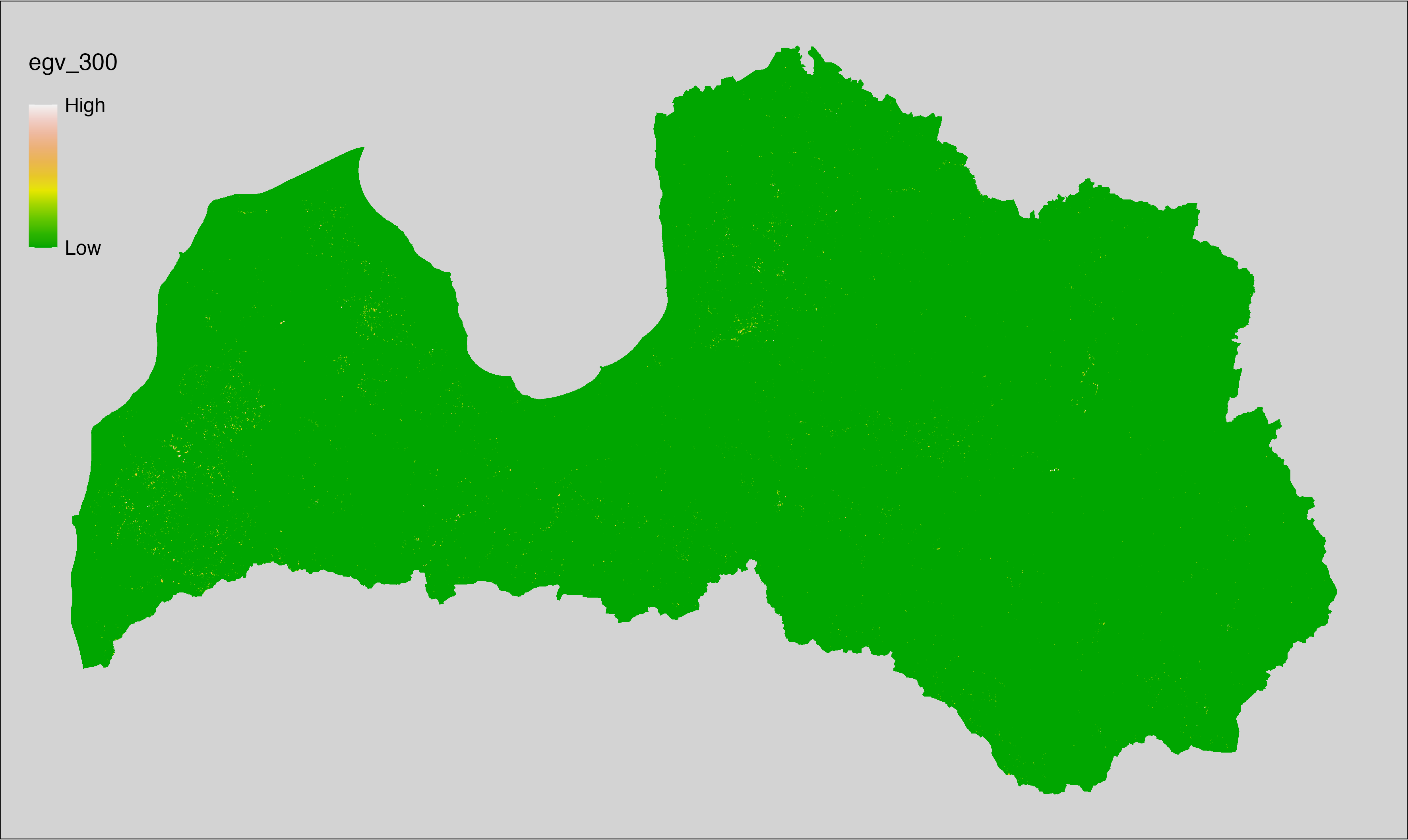
6.301 ForestsQuant_VolumeOakMaple-sum_cell
filename: ForestsQuant_VolumeOakMaple-sum_cell.tif
layername: egv_301
English name: Timber volume of Oaks, Maples within the analysis cell (1 ha)
Latvian name: Ozolu, kļavu krāja analīzes šūnā (1 ha)
Procedure: Most EGVs describing forests are spatially restricted to areas outside of clearcuts and dead stands. This mask is created using a combination of the State Forest Service’s State Forest Registry land category 12 and 14, and The Global Forest Watch pixels classified as lost tree canopy cover since 2020 (raster layer matching input, presence = 1, absence = 0).
This EGV is prepared based on the information of timber volume of oaks and maples (species codes: 10, 61, 24, 63; see tree species codes in Terminology and acronyms) in the inventoried forest stands - State Forest Service’s State Forest Registry. This attribute has some extreme values. We chose to limit them to the nearest integer showing only minimal accumulation in histogram.
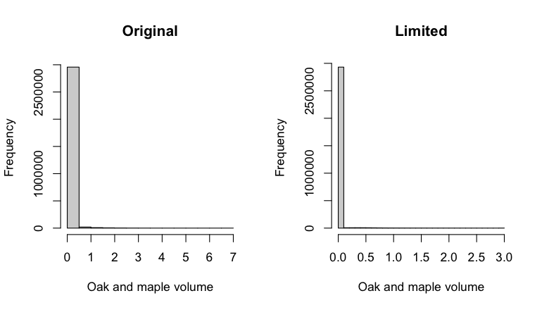
Resulting values at polygon geometries are rasterised with the workflow
egvtools::polygon2input(), restricting to pixels outside the clearcut mask. No
background values are assigned during rasterisation. The resulting layer is
then aggregated to EGV resolution using the workflow egvtools::input2egv() by calculating
sum of pixel values. After the aggregation, cells with no forest information
are filled with value 0. Finally, the layer is standardised by subtracting
the arithmetic mean and dividing by the root mean squared error.
Code
# libs ----
if(!require(egvtools)) {remotes::install_github("aavotins/egvtools"); require(egvtools)}
if(!require(terra)) {install.packages("terra"); require(terra)}
if(!require(sf)) {install.packages("sf"); require(sf)}
if(!require(tidyverse)) {install.packages("tidyverse"); require(tidyverse)}
if(!require(sfarrow)) {install.packages("sfarrow"); require(sfarrow)}
if(!require(readxl)) {install.packages("readxl"); require(readxl)}
if(!require(raster)) {install.packages("raster"); require(raster)}
if(!require(fasterize)) {install.packages("fasterize"); require(fasterize)}
# templates ----
template100=rast("./Templates/TemplateRasters/LV100m_10km.tif")
template10=rast("./Templates/TemplateRasters/LV10m_10km.tif")
rastrs10=raster(template10)
nulls10=rast("./Templates/TemplateRasters/nulls_LV10m_10km.tif")
nulls100=rast("./Templates/TemplateRasters/nulls_LV100m_10km.tif")
# simple landscape ----
simple_landscape=rast("RasterGrids_10m/2024/Ainava_vienk_mask.tif")
# mvr ----
mvr=st_read_parquet("./Geodata/2024/MVR/nogabali_2024janv.parquet")
mvr$yes=1
# clear cut mask ----
izcirtumi=mvr %>%
filter(zkat %in% c("12","14")) %>%
dplyr::select(yes)
r_izcirtumi_mvr=fasterize(izcirtumi,rastrs10,field="yes")
t_izcirtumi_mvr=rast(r_izcirtumi_mvr)
plot(t_izcirtumi_mvr)
tcl=rast("./Geodata/2024/Trees/GFW/TreeCoverLoss_v1_12.tif")
tcl2=ifel(tcl<20,0,1)
tclX=cover(tcl2,nulls10)
plot(tclX)
clearcut_mask=cover(t_izcirtumi_mvr,tclX,
filename="./RasterGrids_10m/2024/Mask_clearcuts.tif",
overwrite=TRUE)
plot(clearcut_mask)
rm(izcirtumi)
rm(r_izcirtumi_mvr)
rm(t_izcirtumi_mvr)
rm(tcl)
rm(tcl2)
rm(tclX)
# ForestsQuant_VolumeOakMaple-sum_cell.tif egv_301 ----
ozolklavas=c("10","61","24","63")
nogabali=mvr %>%
mutate(OzolKlavuKraja=ifelse(s10 %in% ozolklavas, v10, 0)+ifelse(s11 %in% ozolklavas,v11,0)+
ifelse(s12 %in% ozolklavas, v12,0)+ifelse(s13 %in% ozolklavas,v13,0)+
ifelse(s14 %in% ozolklavas, v14,0)) %>%
mutate(OzolKlavuKraja2=OzolKlavuKraja/10000*10*10) %>%
mutate(OzolKlavuKraja3=ifelse(OzolKlavuKraja2>3,3,OzolKlavuKraja2)) %>%
filter(!is.na(OzolKlavuKraja2))
par(mfrow=c(1,2))
options(scipen=999)
hist(nogabali$OzolKlavuKraja2,main="Original",xlab="Oak and maple volume")
hist(nogabali$OzolKlavuKraja3,main="Limited",xlab="Oak and maple volume")
par(mfrow=c(1,1))
options(scipen=0)
p2i_rez=polygon2input(vector_data=nogabali,
template_path = "./Templates/TemplateRasters/LV10m_10km.tif",
out_path = "./RasterGrids_10m/2024/",
file_name = "ForestsQuant_VolumeOakMaple.tif",
value_field = "OzolKlavuKraja3",
fun="max",
prepare=FALSE,
restrict_to = clearcut_mask,
restrict_values = 0,
plot_result=TRUE,
overwrite=TRUE)
p2i_rez
i2e_rez=input2egv(input="./RasterGrids_10m/2024/ForestsQuant_VolumeOakMaple.tif",
egv_template = "./Templates/TemplateRasters/LV100m_10km.tif",
summary_function = "sum",
missing_job = "CoverOutput",
output_bg = "./Templates/TemplateRasters/nulls_LV100m_10km.tif",
outlocation = "./RasterGrids_100m/2024/RAW/",
outfilename = "ForestsQuant_VolumeOakMaple-sum_cell.tif",
layername = "egv_301",
plot_final=TRUE)
i2e_rez
rm(p2i_rez)
rm(nogabali)
rm(ozolklavas)
rm(i2e_rez)
unlink("./RasterGrids_10m/2024/ForestsQuant_VolumeOakMaple.tif")
# standardisation ----
if(!require(terra)) {install.packages("terra"); require(terra)}
if(!require(tidyverse)) {install.packages("tidyverse"); require(tidyverse)}
nosaukums="ForestsQuant_VolumeOakMaple-sum_cell.tif"
ielasisanas_cels=paste0("./RasterGrids_100m/2024/RAW/",nosaukums)
saglabasanas_cels=paste0("./RasterGrids_100m/2024/Scaled/",nosaukums)
slanis=rast(ielasisanas_cels)
videjais=global(slanis,fun="mean",na.rm=TRUE)
centrets=slanis-videjais[,1]
standartnovirze=terra::global(centrets,fun="rms",na.rm=TRUE)
merogots=centrets/standartnovirze[,1]
writeRaster(merogots,
filename=saglabasanas_cels,
overwrite=TRUE)
6.302 ForestsQuant_VolumePine-sum_cell
filename: ForestsQuant_VolumePine-sum_cell.tif
layername: egv_302
English name: Timber volume of Pines within the analysis cell (1 ha)
Latvian name: Priežu krāja analīzes šūnā (1 ha)
Procedure: Most EGVs describing forests are spatially restricted to areas outside of clearcuts and dead stands. This mask is created using a combination of the State Forest Service’s State Forest Registry land category 12 and 14, and The Global Forest Watch pixels classified as lost tree canopy cover since 2020 (raster layer matching input, presence = 1, absence = 0).
This EGV is prepared based on the information of timber volume of pines (species codes: 1, 14, 22; see tree species codes in Terminology and acronyms) in the inventoried forest stands - State Forest Service’s State Forest Registry. This attribute has some extreme values. We chose to limit them to the nearest integer showing only minimal accumulation in histogram.
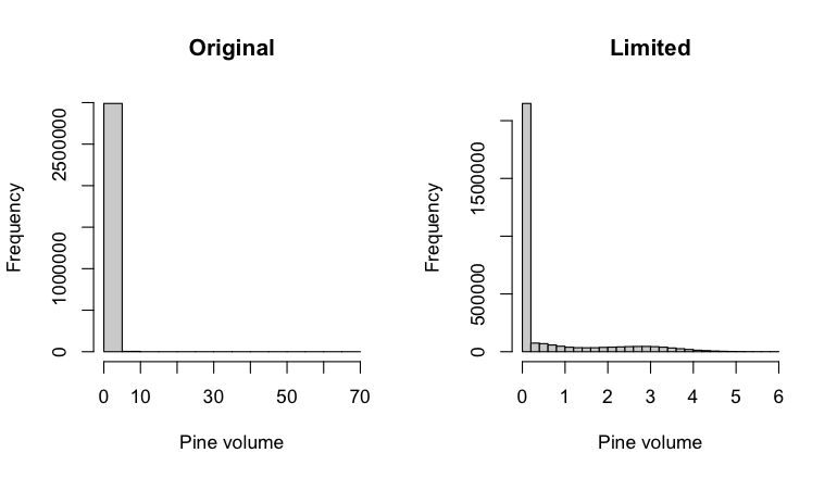
Resulting values at polygon geometries are rasterised with the workflow
egvtools::polygon2input(), restricting to pixels outside the clearcut mask. No
background values are assigned during rasterisation. The resulting layer is
then aggregated to EGV resolution using the workflow egvtools::input2egv() by calculating
sum of pixel values. After the aggregation, cells with no forest information
are filled with value 0. Finally, the layer is standardised by subtracting
the arithmetic mean and dividing by the root mean squared error.
Code
# libs ----
if(!require(egvtools)) {remotes::install_github("aavotins/egvtools"); require(egvtools)}
if(!require(terra)) {install.packages("terra"); require(terra)}
if(!require(sf)) {install.packages("sf"); require(sf)}
if(!require(tidyverse)) {install.packages("tidyverse"); require(tidyverse)}
if(!require(sfarrow)) {install.packages("sfarrow"); require(sfarrow)}
if(!require(readxl)) {install.packages("readxl"); require(readxl)}
if(!require(raster)) {install.packages("raster"); require(raster)}
if(!require(fasterize)) {install.packages("fasterize"); require(fasterize)}
# templates ----
template100=rast("./Templates/TemplateRasters/LV100m_10km.tif")
template10=rast("./Templates/TemplateRasters/LV10m_10km.tif")
rastrs10=raster(template10)
nulls10=rast("./Templates/TemplateRasters/nulls_LV10m_10km.tif")
nulls100=rast("./Templates/TemplateRasters/nulls_LV100m_10km.tif")
# simple landscape ----
simple_landscape=rast("RasterGrids_10m/2024/Ainava_vienk_mask.tif")
# mvr ----
mvr=st_read_parquet("./Geodata/2024/MVR/nogabali_2024janv.parquet")
mvr$yes=1
# clear cut mask ----
izcirtumi=mvr %>%
filter(zkat %in% c("12","14")) %>%
dplyr::select(yes)
r_izcirtumi_mvr=fasterize(izcirtumi,rastrs10,field="yes")
t_izcirtumi_mvr=rast(r_izcirtumi_mvr)
plot(t_izcirtumi_mvr)
tcl=rast("./Geodata/2024/Trees/GFW/TreeCoverLoss_v1_12.tif")
tcl2=ifel(tcl<20,0,1)
tclX=cover(tcl2,nulls10)
plot(tclX)
clearcut_mask=cover(t_izcirtumi_mvr,tclX,
filename="./RasterGrids_10m/2024/Mask_clearcuts.tif",
overwrite=TRUE)
plot(clearcut_mask)
rm(izcirtumi)
rm(r_izcirtumi_mvr)
rm(t_izcirtumi_mvr)
rm(tcl)
rm(tcl2)
rm(tclX)
# ForestsQuant_VolumePine-sum_cell.tif egv_302 ----
priedes=c("1","14","22")
nogabali=mvr %>%
mutate(PriezuKraja=ifelse(s10 %in% priedes, v10, 0)+ifelse(s11 %in% priedes,v11,0)+
ifelse(s12 %in% priedes, v12,0)+ifelse(s13 %in% priedes,v13,0)+
ifelse(s14 %in% priedes, v14,0)) %>%
mutate(PriezuKraja2=PriezuKraja/10000*10*10) %>%
mutate(PriezuKraja3=ifelse(PriezuKraja2>6,6,PriezuKraja2)) %>%
filter(!is.na(PriezuKraja2))
par(mfrow=c(1,2))
options(scipen=999)
hist(nogabali$PriezuKraja2,main="Original",xlab="Pine volume")
hist(nogabali$PriezuKraja3,main="Limited",xlab="Pine volume")
par(mfrow=c(1,1))
options(scipen=0)
p2i_rez=polygon2input(vector_data=nogabali,
template_path = "./Templates/TemplateRasters/LV10m_10km.tif",
out_path = "./RasterGrids_10m/2024/",
file_name = "ForestsQuant_VolumePine.tif",
value_field = "PriezuKraja3",
fun="max",
prepare=FALSE,
restrict_to = clearcut_mask,
restrict_values = 0,
plot_result=TRUE,
overwrite=TRUE)
p2i_rez
i2e_rez=input2egv(input="./RasterGrids_10m/2024/ForestsQuant_VolumePine.tif",
egv_template = "./Templates/TemplateRasters/LV100m_10km.tif",
summary_function = "sum",
missing_job = "CoverOutput",
output_bg = "./Templates/TemplateRasters/nulls_LV100m_10km.tif",
outlocation = "./RasterGrids_100m/2024/RAW/",
outfilename = "ForestsQuant_VolumePine-sum_cell.tif",
layername = "egv_302",
plot_final=TRUE)
i2e_rez
rm(p2i_rez)
rm(nogabali)
rm(priedes)
rm(i2e_rez)
unlink("./RasterGrids_10m/2024/ForestsQuant_VolumePine.tif")
# standardisation ----
if(!require(terra)) {install.packages("terra"); require(terra)}
if(!require(tidyverse)) {install.packages("tidyverse"); require(tidyverse)}
nosaukums="ForestsQuant_VolumePine-sum_cell.tif"
ielasisanas_cels=paste0("./RasterGrids_100m/2024/RAW/",nosaukums)
saglabasanas_cels=paste0("./RasterGrids_100m/2024/Scaled/",nosaukums)
slanis=rast(ielasisanas_cels)
videjais=global(slanis,fun="mean",na.rm=TRUE)
centrets=slanis-videjais[,1]
standartnovirze=terra::global(centrets,fun="rms",na.rm=TRUE)
merogots=centrets/standartnovirze[,1]
writeRaster(merogots,
filename=saglabasanas_cels,
overwrite=TRUE)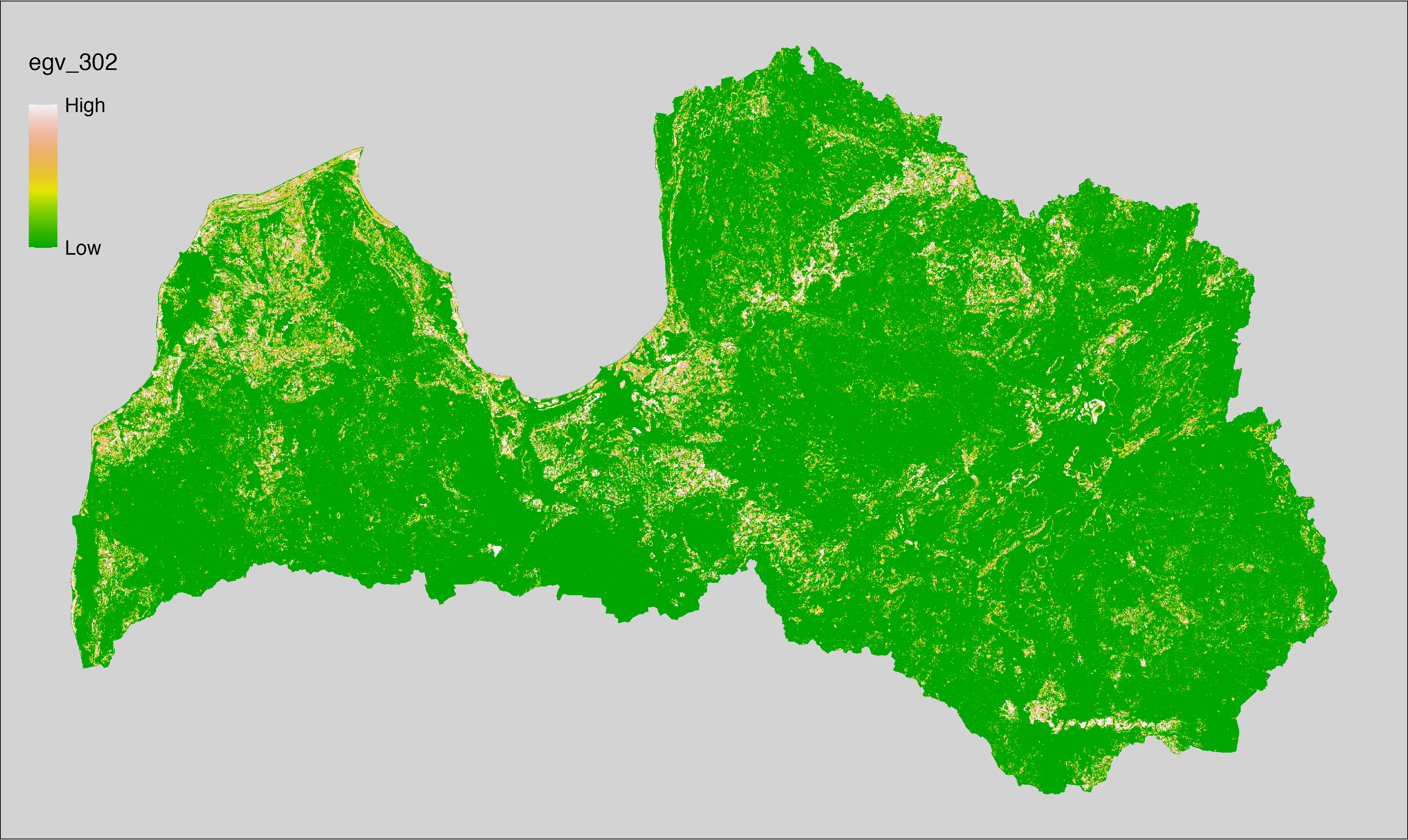
6.303 ForestsQuant_VolumeSpruce-sum_cell
filename: ForestsQuant_VolumeSpruce-sum_cell.tif
layername: egv_303
English name: Timber volume of Spruces within the analysis cell (1 ha)
Latvian name: Egļu krāja analīzes šūnā (1 ha)
Procedure: Most EGVs describing forests are spatially restricted to areas outside of clearcuts and dead stands. This mask is created using a combination of the State Forest Service’s State Forest Registry land category 12 and 14, and The Global Forest Watch pixels classified as lost tree canopy cover since 2020 (raster layer matching input, presence = 1, absence = 0).
This EGV is prepared based on the information of timber volume of spruces
(species codes: 3, 13, 15, 23, 28; see tree species codes in Terminology and
acronyms) in the inventoried forest stands - State Forest Service’s
State Forest Registry. This attribute has some extreme
values. We chose to limit them to the nearest integer showing only minimal
accumulation in histogram.
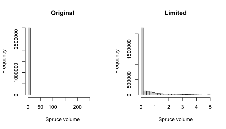
Resulting values at polygon geometries are rasterised with the workflow
egvtools::polygon2input(), restricting to pixels outside the clearcut mask. No
background values are assigned during rasterisation. The resulting layer is
then aggregated to EGV resolution using the workflow egvtools::input2egv() by calculating
sum of pixel values. After the aggregation, cells with no forest information
are filled with value 0. Finally, the layer is standardised by subtracting
the arithmetic mean and dividing by the root mean squared error.
Code
# libs ----
if(!require(egvtools)) {remotes::install_github("aavotins/egvtools"); require(egvtools)}
if(!require(terra)) {install.packages("terra"); require(terra)}
if(!require(sf)) {install.packages("sf"); require(sf)}
if(!require(tidyverse)) {install.packages("tidyverse"); require(tidyverse)}
if(!require(sfarrow)) {install.packages("sfarrow"); require(sfarrow)}
if(!require(readxl)) {install.packages("readxl"); require(readxl)}
if(!require(raster)) {install.packages("raster"); require(raster)}
if(!require(fasterize)) {install.packages("fasterize"); require(fasterize)}
# templates ----
template100=rast("./Templates/TemplateRasters/LV100m_10km.tif")
template10=rast("./Templates/TemplateRasters/LV10m_10km.tif")
rastrs10=raster(template10)
nulls10=rast("./Templates/TemplateRasters/nulls_LV10m_10km.tif")
nulls100=rast("./Templates/TemplateRasters/nulls_LV100m_10km.tif")
# simple landscape ----
simple_landscape=rast("RasterGrids_10m/2024/Ainava_vienk_mask.tif")
# mvr ----
mvr=st_read_parquet("./Geodata/2024/MVR/nogabali_2024janv.parquet")
mvr$yes=1
# clear cut mask ----
izcirtumi=mvr %>%
filter(zkat %in% c("12","14")) %>%
dplyr::select(yes)
r_izcirtumi_mvr=fasterize(izcirtumi,rastrs10,field="yes")
t_izcirtumi_mvr=rast(r_izcirtumi_mvr)
plot(t_izcirtumi_mvr)
tcl=rast("./Geodata/2024/Trees/GFW/TreeCoverLoss_v1_12.tif")
tcl2=ifel(tcl<20,0,1)
tclX=cover(tcl2,nulls10)
plot(tclX)
clearcut_mask=cover(t_izcirtumi_mvr,tclX,
filename="./RasterGrids_10m/2024/Mask_clearcuts.tif",
overwrite=TRUE)
plot(clearcut_mask)
rm(izcirtumi)
rm(r_izcirtumi_mvr)
rm(t_izcirtumi_mvr)
rm(tcl)
rm(tcl2)
rm(tclX)
# ForestsQuant_VolumeSpruce-sum_cell.tif egv_303 ----
egles=c("3","13","15","23","28")
nogabali=mvr %>%
mutate(EgluKraja=ifelse(s10 %in% egles, v10, 0)+ifelse(s11 %in% egles,v11,0)+
ifelse(s12 %in% egles, v12,0)+ifelse(s13 %in% egles,v13,0)+
ifelse(s14 %in% egles, v14,0)) %>%
mutate(EgluKraja2=EgluKraja/10000*10*10) %>%
mutate(EgluKraja3=ifelse(EgluKraja2>5,5,EgluKraja2)) %>%
filter(!is.na(EgluKraja2))
par(mfrow=c(1,2))
options(scipen=999)
hist(nogabali$EgluKraja2,main="Original",xlab="Spruce volume")
hist(nogabali$EgluKraja3,main="Limited",xlab="Spruce volume")
par(mfrow=c(1,1))
options(scipen=0)
p2i_rez=polygon2input(vector_data=nogabali,
template_path = "./Templates/TemplateRasters/LV10m_10km.tif",
out_path = "./RasterGrids_10m/2024/",
file_name = "ForestsQuant_VolumeSpruce.tif",
value_field = "EgluKraja3",
fun="max",
prepare=FALSE,
restrict_to = clearcut_mask,
restrict_values = 0,
plot_result=TRUE,
overwrite=TRUE)
p2i_rez
i2e_rez=input2egv(input="./RasterGrids_10m/2024/ForestsQuant_VolumeSpruce.tif",
egv_template = "./Templates/TemplateRasters/LV100m_10km.tif",
summary_function = "sum",
missing_job = "CoverOutput",
output_bg = "./Templates/TemplateRasters/nulls_LV100m_10km.tif",
outlocation = "./RasterGrids_100m/2024/RAW/",
outfilename = "ForestsQuant_VolumeSpruce-sum_cell.tif",
layername = "egv_303",
plot_final=TRUE)
i2e_rez
rm(p2i_rez)
rm(nogabali)
rm(egles)
rm(i2e_rez)
unlink("./RasterGrids_10m/2024/ForestsQuant_VolumeSpruce.tif")
# standardisation ----
if(!require(terra)) {install.packages("terra"); require(terra)}
if(!require(tidyverse)) {install.packages("tidyverse"); require(tidyverse)}
nosaukums="ForestsQuant_VolumeSpruce-sum_cell.tif"
ielasisanas_cels=paste0("./RasterGrids_100m/2024/RAW/",nosaukums)
saglabasanas_cels=paste0("./RasterGrids_100m/2024/Scaled/",nosaukums)
slanis=rast(ielasisanas_cels)
videjais=global(slanis,fun="mean",na.rm=TRUE)
centrets=slanis-videjais[,1]
standartnovirze=terra::global(centrets,fun="rms",na.rm=TRUE)
merogots=centrets/standartnovirze[,1]
writeRaster(merogots,
filename=saglabasanas_cels,
overwrite=TRUE)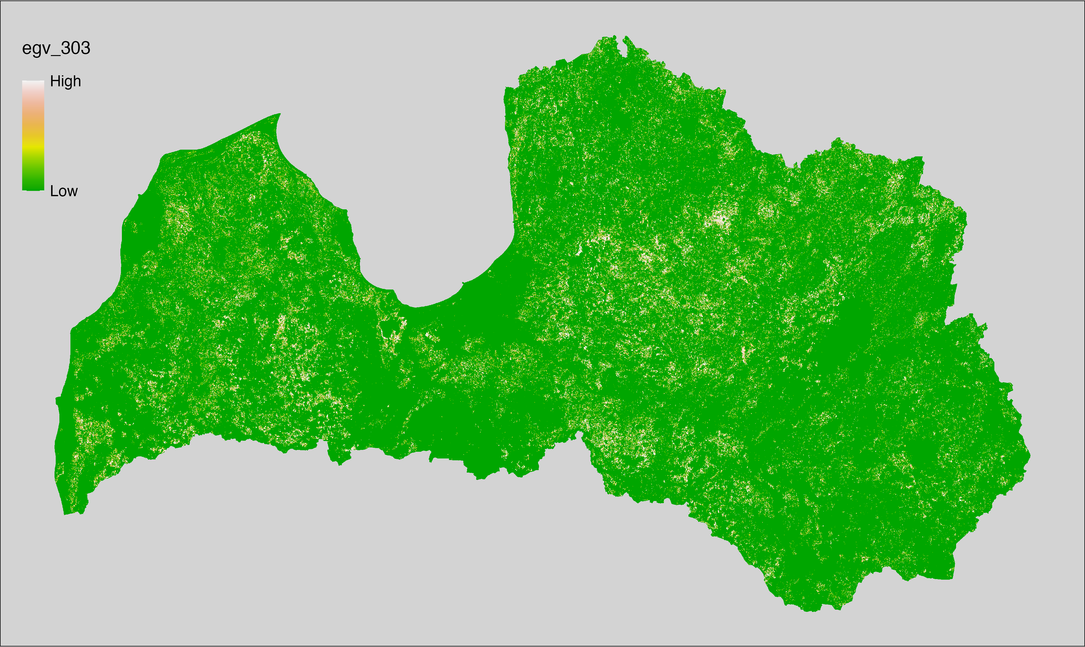
6.304 ForestsQuant_VolumeTemperateDeciduousTotal-sum_cell
filename: ForestsQuant_VolumeTemperateDeciduousTotal-sum_cell.tif
layername: egv_304
English name: Timber volume of Temperate Deciduous trees within the analysis cell (1 ha)
Latvian name: Platlapju krāja analīzes šūnā (1 ha)
Procedure: Most EGVs describing forests are spatially restricted to areas outside of clearcuts and dead stands. This mask is created using a combination of the State Forest Service’s State Forest Registry land category 12 and 14, and The Global Forest Watch pixels classified as lost tree canopy cover since 2020 (raster layer matching input, presence = 1, absence = 0).
This EGV is prepared based on the information of timber volume of temperate deciduous tree species (species codes: 10, 11, 12, 16, 17, 18, 24, 25, 26, 27, 29, 50, 61, 62, 63, 64, 65, 66, 67, 69; see tree species codes in Terminology and acronyms) in the inventoried forest stands - State Forest Service’s State Forest Registry. This attribute has some extreme values. We chose to limit them to the nearest integer showing only minimal accumulation in histogram.
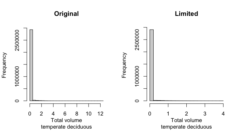
Resulting values at polygon geometries are rasterised with the workflow
egvtools::polygon2input(), restricting to pixels outside the clearcut mask. No
background values are assigned during rasterisation. The resulting layer is
then aggregated to EGV resolution using the workflow egvtools::input2egv() by calculating
sum of pixel values. After the aggregation, cells with no forest information
are filled with value 0. Finally, the layer is standardised by subtracting
the arithmetic mean and dividing by the root mean squared error.
Code
# libs ----
if(!require(egvtools)) {remotes::install_github("aavotins/egvtools"); require(egvtools)}
if(!require(terra)) {install.packages("terra"); require(terra)}
if(!require(sf)) {install.packages("sf"); require(sf)}
if(!require(tidyverse)) {install.packages("tidyverse"); require(tidyverse)}
if(!require(sfarrow)) {install.packages("sfarrow"); require(sfarrow)}
if(!require(readxl)) {install.packages("readxl"); require(readxl)}
if(!require(raster)) {install.packages("raster"); require(raster)}
if(!require(fasterize)) {install.packages("fasterize"); require(fasterize)}
# templates ----
template100=rast("./Templates/TemplateRasters/LV100m_10km.tif")
template10=rast("./Templates/TemplateRasters/LV10m_10km.tif")
rastrs10=raster(template10)
nulls10=rast("./Templates/TemplateRasters/nulls_LV10m_10km.tif")
nulls100=rast("./Templates/TemplateRasters/nulls_LV100m_10km.tif")
# simple landscape ----
simple_landscape=rast("RasterGrids_10m/2024/Ainava_vienk_mask.tif")
# mvr ----
mvr=st_read_parquet("./Geodata/2024/MVR/nogabali_2024janv.parquet")
mvr$yes=1
# clear cut mask ----
izcirtumi=mvr %>%
filter(zkat %in% c("12","14")) %>%
dplyr::select(yes)
r_izcirtumi_mvr=fasterize(izcirtumi,rastrs10,field="yes")
t_izcirtumi_mvr=rast(r_izcirtumi_mvr)
plot(t_izcirtumi_mvr)
tcl=rast("./Geodata/2024/Trees/GFW/TreeCoverLoss_v1_12.tif")
tcl2=ifel(tcl<20,0,1)
tclX=cover(tcl2,nulls10)
plot(tclX)
clearcut_mask=cover(t_izcirtumi_mvr,tclX,
filename="./RasterGrids_10m/2024/Mask_clearcuts.tif",
overwrite=TRUE)
plot(clearcut_mask)
rm(izcirtumi)
rm(r_izcirtumi_mvr)
rm(t_izcirtumi_mvr)
rm(tcl)
rm(tcl2)
rm(tclX)
# ForestsQuant_VolumeTemperateDeciduousTotal-sum_cell.tif egv_304 ----
platlapji=c("10","11","12","16","17","18","24","25","26","27","29","50",
"61","62","63","64","65","66","67","69")
nogabali=mvr %>%
mutate(PlatKraja=ifelse(s10 %in% platlapji, v10, 0)+ifelse(s11 %in% platlapji,v11,0)+
ifelse(s12 %in% platlapji, v12,0)+ifelse(s13 %in% platlapji,v13,0)+
ifelse(s14 %in% platlapji, v14,0)) %>%
mutate(PlatKraja2=PlatKraja/10000*10*10) %>%
mutate(PlatKraja3=ifelse(PlatKraja2>4,4,PlatKraja2)) %>%
filter(!is.na(PlatKraja2))
par(mfrow=c(1,2))
options(scipen=999)
hist(nogabali$PlatKraja2,main="Original",xlab="Total volume\ntemperate deciduous")
hist(nogabali$PlatKraja3,main="Limited",xlab="Total volume\ntemperate deciduous")
par(mfrow=c(1,1))
options(scipen=0)
p2i_rez=polygon2input(vector_data=nogabali,
template_path = "./Templates/TemplateRasters/LV10m_10km.tif",
out_path = "./RasterGrids_10m/2024/",
file_name = "ForestsQuant_VolumeTemperateDeciduousTotal.tif",
value_field = "PlatKraja3",
fun="max",
prepare=FALSE,
restrict_to = clearcut_mask,
restrict_values = 0,
plot_result=TRUE,
overwrite=TRUE)
p2i_rez
i2e_rez=input2egv(input="./RasterGrids_10m/2024/ForestsQuant_VolumeTemperateDeciduousTotal.tif",
egv_template = "./Templates/TemplateRasters/LV100m_10km.tif",
summary_function = "sum",
missing_job = "CoverOutput",
output_bg = "./Templates/TemplateRasters/nulls_LV100m_10km.tif",
outlocation = "./RasterGrids_100m/2024/RAW/",
outfilename = "ForestsQuant_VolumeTemperateDeciduousTotal-sum_cell.tif",
layername = "egv_304",
plot_final=TRUE)
i2e_rez
rm(p2i_rez)
rm(nogabali)
rm(platlapji)
rm(i2e_rez)
unlink("./RasterGrids_10m/2024/ForestsQuant_VolumeTemperateDeciduousTotal.tif")
# standardisation ----
if(!require(terra)) {install.packages("terra"); require(terra)}
if(!require(tidyverse)) {install.packages("tidyverse"); require(tidyverse)}
nosaukums="ForestsQuant_VolumeTemperateDeciduousTotal-sum_cell.tif"
ielasisanas_cels=paste0("./RasterGrids_100m/2024/RAW/",nosaukums)
saglabasanas_cels=paste0("./RasterGrids_100m/2024/Scaled/",nosaukums)
slanis=rast(ielasisanas_cels)
videjais=global(slanis,fun="mean",na.rm=TRUE)
centrets=slanis-videjais[,1]
standartnovirze=terra::global(centrets,fun="rms",na.rm=TRUE)
merogots=centrets/standartnovirze[,1]
writeRaster(merogots,
filename=saglabasanas_cels,
overwrite=TRUE)
6.305 ForestsQuant_VolumeTemperateWithoutOak-sum_cell
filename: ForestsQuant_VolumeTemperateWithoutOak-sum_cell.tif
layername: egv_305
English name: Timber volume of Temperate Deciduous trees (without oaks) within the analysis cell (1 ha)
Latvian name: Platlapju (bez ozoliem) krāja analīzes šūnā (1 ha)
Procedure: Most EGVs describing forests are spatially restricted to areas outside of clearcuts and dead stands. This mask is created using a combination of the State Forest Service’s State Forest Registry land category 12 and 14, and The Global Forest Watch pixels classified as lost tree canopy cover since 2020 (raster layer matching input, presence = 1, absence = 0).
This EGV is prepared based on the information of timber volume of temperate deciduous tree species except oaks (species codes: 11, 12, 16, 17, 18, 24, 25, 26, 27, 29, 50, 62, 63, 64, 65, 66, 67, 69; see tree species codes in Terminology and acronyms) in the inventoried forest stands - State Forest Service’s State Forest Registry. This attribute has some extreme values. We chose to limit them to the nearest integer showing only minimal accumulation in histogram.
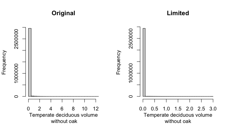
Resulting values at polygon geometries are rasterised with the workflow
egvtools::polygon2input(), restricting to pixels outside the clearcut mask. No
background values are assigned during rasterisation. The resulting layer is
then aggregated to EGV resolution using the workflow egvtools::input2egv() by calculating
sum of pixel values. After the aggregation, cells with no forest information
are filled with value 0. Finally, the layer is standardised by subtracting
the arithmetic mean and dividing by the root mean squared error.
Code
# libs ----
if(!require(egvtools)) {remotes::install_github("aavotins/egvtools"); require(egvtools)}
if(!require(terra)) {install.packages("terra"); require(terra)}
if(!require(sf)) {install.packages("sf"); require(sf)}
if(!require(tidyverse)) {install.packages("tidyverse"); require(tidyverse)}
if(!require(sfarrow)) {install.packages("sfarrow"); require(sfarrow)}
if(!require(readxl)) {install.packages("readxl"); require(readxl)}
if(!require(raster)) {install.packages("raster"); require(raster)}
if(!require(fasterize)) {install.packages("fasterize"); require(fasterize)}
# templates ----
template100=rast("./Templates/TemplateRasters/LV100m_10km.tif")
template10=rast("./Templates/TemplateRasters/LV10m_10km.tif")
rastrs10=raster(template10)
nulls10=rast("./Templates/TemplateRasters/nulls_LV10m_10km.tif")
nulls100=rast("./Templates/TemplateRasters/nulls_LV100m_10km.tif")
# simple landscape ----
simple_landscape=rast("RasterGrids_10m/2024/Ainava_vienk_mask.tif")
# mvr ----
mvr=st_read_parquet("./Geodata/2024/MVR/nogabali_2024janv.parquet")
mvr$yes=1
# clear cut mask ----
izcirtumi=mvr %>%
filter(zkat %in% c("12","14")) %>%
dplyr::select(yes)
r_izcirtumi_mvr=fasterize(izcirtumi,rastrs10,field="yes")
t_izcirtumi_mvr=rast(r_izcirtumi_mvr)
plot(t_izcirtumi_mvr)
tcl=rast("./Geodata/2024/Trees/GFW/TreeCoverLoss_v1_12.tif")
tcl2=ifel(tcl<20,0,1)
tclX=cover(tcl2,nulls10)
plot(tclX)
clearcut_mask=cover(t_izcirtumi_mvr,tclX,
filename="./RasterGrids_10m/2024/Mask_clearcuts.tif",
overwrite=TRUE)
plot(clearcut_mask)
rm(izcirtumi)
rm(r_izcirtumi_mvr)
rm(t_izcirtumi_mvr)
rm(tcl)
rm(tcl2)
rm(tclX)
# ForestsQuant_VolumeTemperateWithoutOak-sum_cell.tif egv_305 ----
neozoli=c("11","12","16","17","18","24","25","26","27","29","50",
"62","63","64","65","66","67","69")
nogabali=mvr %>%
mutate(BezOzoluKraja=ifelse(s10 %in% neozoli, v10, 0)+ifelse(s11 %in% neozoli,v11,0)+
ifelse(s12 %in% neozoli, v12,0)+ifelse(s13 %in% neozoli,v13,0)+
ifelse(s14 %in% neozoli, v14,0)) %>%
mutate(BezOzoluKraja2=BezOzoluKraja/10000*10*10) %>%
mutate(BezOzoluKraja3=ifelse(BezOzoluKraja2>3,3,BezOzoluKraja2)) %>%
filter(!is.na(BezOzoluKraja2))
par(mfrow=c(1,2))
options(scipen=999)
hist(nogabali$BezOzoluKraja2,main="Original",xlab="Temperate deciduous volume\n without oak")
hist(nogabali$BezOzoluKraja3,main="Limited",xlab="Temperate deciduous volume\nwithout oak")
par(mfrow=c(1,1))
options(scipen=0)
p2i_rez=polygon2input(vector_data=nogabali,
template_path = "./Templates/TemplateRasters/LV10m_10km.tif",
out_path = "./RasterGrids_10m/2024/",
file_name = "ForestsQuant_VolumeTemperateWithoutOak.tif",
value_field = "BezOzoluKraja3",
fun="max",
prepare=FALSE,
restrict_to = clearcut_mask,
restrict_values = 0,
plot_result=TRUE,
overwrite=TRUE)
p2i_rez
i2e_rez=input2egv(input="./RasterGrids_10m/2024/ForestsQuant_VolumeTemperateWithoutOak.tif",
egv_template = "./Templates/TemplateRasters/LV100m_10km.tif",
summary_function = "sum",
missing_job = "CoverOutput",
output_bg = "./Templates/TemplateRasters/nulls_LV100m_10km.tif",
outlocation = "./RasterGrids_100m/2024/RAW/",
outfilename = "ForestsQuant_VolumeTemperateWithoutOak-sum_cell.tif",
layername = "egv_305",
plot_final=TRUE)
i2e_rez
rm(p2i_rez)
rm(nogabali)
rm(neozoli)
rm(i2e_rez)
unlink("./RasterGrids_10m/2024/ForestsQuant_VolumeTemperateWithoutOak.tif")
# standardisation ----
if(!require(terra)) {install.packages("terra"); require(terra)}
if(!require(tidyverse)) {install.packages("tidyverse"); require(tidyverse)}
nosaukums="ForestsQuant_VolumeTemperateWithoutOak-sum_cell.tif"
ielasisanas_cels=paste0("./RasterGrids_100m/2024/RAW/",nosaukums)
saglabasanas_cels=paste0("./RasterGrids_100m/2024/Scaled/",nosaukums)
slanis=rast(ielasisanas_cels)
videjais=global(slanis,fun="mean",na.rm=TRUE)
centrets=slanis-videjais[,1]
standartnovirze=terra::global(centrets,fun="rms",na.rm=TRUE)
merogots=centrets/standartnovirze[,1]
writeRaster(merogots,
filename=saglabasanas_cels,
overwrite=TRUE)
6.306 ForestsQuant_VolumeTemperateWithoutOakMaple-sum_cell
filename: ForestsQuant_VolumeTemperateWithoutOakMaple-sum_cell.tif
layername: egv_306
English name: Timber volume of Temperate Deciduous trees (without oaks, maples) within the analysis cell (1 ha)
Latvian name: Platlapju (bez ozoliem, kļavām) krāja analīzes šūnā (1 ha)
Procedure: Most EGVs describing forests are spatially restricted to areas outside of clearcuts and dead stands. This mask is created using a combination of the State Forest Service’s State Forest Registry land category 12 and 14, and The Global Forest Watch pixels classified as lost tree canopy cover since 2020 (raster layer matching input, presence = 1, absence = 0).
This EGV is prepared based on the information of timber volume of teperate deciduous trees except oaks and maples (species codes: 11, 12, 16, 17, 18, 25, 26, 27, 29, 50, 62, 64, 65, 66, 67, 69; see tree species codes in Terminology and acronyms) in the inventoried forest stands - State Forest Service’s State Forest Registry. This attribute has some extreme values. We chose to limit them to the nearest integer showing only minimal accumulation in histogram.
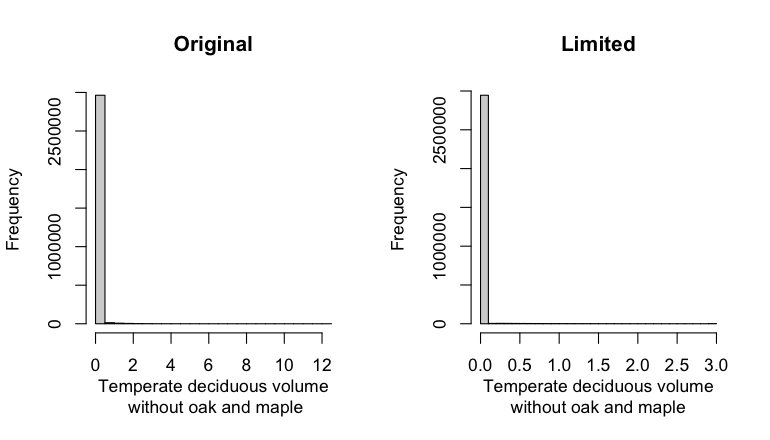
Resulting values at polygon geometries are rasterised with the workflow
egvtools::polygon2input(), restricting to pixels outside the clearcut mask. No
background values are assigned during rasterisation. The resulting layer is
then aggregated to EGV resolution using the workflow egvtools::input2egv() by calculating
sum of pixel values. After the aggregation, cells with no forest information
are filled with value 0. Finally, the layer is standardised by subtracting
the arithmetic mean and dividing by the root mean squared error.
Code
# libs ----
if(!require(egvtools)) {remotes::install_github("aavotins/egvtools"); require(egvtools)}
if(!require(terra)) {install.packages("terra"); require(terra)}
if(!require(sf)) {install.packages("sf"); require(sf)}
if(!require(tidyverse)) {install.packages("tidyverse"); require(tidyverse)}
if(!require(sfarrow)) {install.packages("sfarrow"); require(sfarrow)}
if(!require(readxl)) {install.packages("readxl"); require(readxl)}
if(!require(raster)) {install.packages("raster"); require(raster)}
if(!require(fasterize)) {install.packages("fasterize"); require(fasterize)}
# templates ----
template100=rast("./Templates/TemplateRasters/LV100m_10km.tif")
template10=rast("./Templates/TemplateRasters/LV10m_10km.tif")
rastrs10=raster(template10)
nulls10=rast("./Templates/TemplateRasters/nulls_LV10m_10km.tif")
nulls100=rast("./Templates/TemplateRasters/nulls_LV100m_10km.tif")
# simple landscape ----
simple_landscape=rast("RasterGrids_10m/2024/Ainava_vienk_mask.tif")
# mvr ----
mvr=st_read_parquet("./Geodata/2024/MVR/nogabali_2024janv.parquet")
mvr$yes=1
# clear cut mask ----
izcirtumi=mvr %>%
filter(zkat %in% c("12","14")) %>%
dplyr::select(yes)
r_izcirtumi_mvr=fasterize(izcirtumi,rastrs10,field="yes")
t_izcirtumi_mvr=rast(r_izcirtumi_mvr)
plot(t_izcirtumi_mvr)
tcl=rast("./Geodata/2024/Trees/GFW/TreeCoverLoss_v1_12.tif")
tcl2=ifel(tcl<20,0,1)
tclX=cover(tcl2,nulls10)
plot(tclX)
clearcut_mask=cover(t_izcirtumi_mvr,tclX,
filename="./RasterGrids_10m/2024/Mask_clearcuts.tif",
overwrite=TRUE)
plot(clearcut_mask)
rm(izcirtumi)
rm(r_izcirtumi_mvr)
rm(t_izcirtumi_mvr)
rm(tcl)
rm(tcl2)
rm(tclX)
# ForestsQuant_VolumeTemperateWithoutOakMaple-sum_cell.tif egv_306 ----
neozolklavas=c("11","12","16","17","18","25","26","27","29","50",
"62","64","65","66","67","69")
nogabali=mvr %>%
mutate(BezOzolKlavuKraja=ifelse(s10 %in% neozolklavas, v10, 0)+ifelse(s11 %in% neozolklavas,v11,0)+
ifelse(s12 %in% neozolklavas, v12,0)+ifelse(s13 %in% neozolklavas,v13,0)+
ifelse(s14 %in% neozolklavas, v14,0)) %>%
mutate(BezOzolKlavuKraja2=BezOzolKlavuKraja/10000*10*10) %>%
mutate(BezOzolKlavuKraja3=ifelse(BezOzolKlavuKraja2>3,3,BezOzolKlavuKraja2)) %>%
filter(!is.na(BezOzolKlavuKraja2))
par(mfrow=c(1,2))
options(scipen=999)
hist(nogabali$BezOzolKlavuKraja2,main="Original",xlab="Temperate deciduous volume\n without oak and maple")
hist(nogabali$BezOzolKlavuKraja3,main="Limited",xlab="Temperate deciduous volume\nwithout oak and maple")
par(mfrow=c(1,1))
options(scipen=0)
p2i_rez=polygon2input(vector_data=nogabali,
template_path = "./Templates/TemplateRasters/LV10m_10km.tif",
out_path = "./RasterGrids_10m/2024/",
file_name = "ForestsQuant_VolumeTemperateWithoutOakMaple.tif",
value_field = "BezOzolKlavuKraja3",
fun="max",
prepare=FALSE,
restrict_to = clearcut_mask,
restrict_values = 0,
plot_result=TRUE,
overwrite=TRUE)
p2i_rez
i2e_rez=input2egv(input="./RasterGrids_10m/2024/ForestsQuant_VolumeTemperateWithoutOakMaple.tif",
egv_template = "./Templates/TemplateRasters/LV100m_10km.tif",
summary_function = "sum",
missing_job = "CoverOutput",
output_bg = "./Templates/TemplateRasters/nulls_LV100m_10km.tif",
outlocation = "./RasterGrids_100m/2024/RAW/",
outfilename = "ForestsQuant_VolumeTemperateWithoutOakMaple-sum_cell.tif",
layername = "egv_306",
plot_final=TRUE)
i2e_rez
rm(p2i_rez)
rm(nogabali)
rm(neozolklavas)
rm(i2e_rez)
unlink("./RasterGrids_10m/2024/ForestsQuant_VolumeTemperateWithoutOakMaple.tif")
# standardisation ----
if(!require(terra)) {install.packages("terra"); require(terra)}
if(!require(tidyverse)) {install.packages("tidyverse"); require(tidyverse)}
nosaukums="ForestsQuant_VolumeTemperateWithoutOakMaple-sum_cell.tif"
ielasisanas_cels=paste0("./RasterGrids_100m/2024/RAW/",nosaukums)
saglabasanas_cels=paste0("./RasterGrids_100m/2024/Scaled/",nosaukums)
slanis=rast(ielasisanas_cels)
videjais=global(slanis,fun="mean",na.rm=TRUE)
centrets=slanis-videjais[,1]
standartnovirze=terra::global(centrets,fun="rms",na.rm=TRUE)
merogots=centrets/standartnovirze[,1]
writeRaster(merogots,
filename=saglabasanas_cels,
overwrite=TRUE)
6.307 ForestsQuant_VolumeTotal-sum_cell
filename: ForestsQuant_VolumeTotal-sum_cell.tif
layername: egv_307
English name: Timber volume within the analysis cell (1 ha)
Latvian name: Kopējā krāja analīzes šūnā (1 ha)
Procedure: Most EGVs describing forests are spatially restricted to areas outside of clearcuts and dead stands. This mask is created using a combination of the State Forest Service’s State Forest Registry land category 12 and 14, and The Global Forest Watch pixels classified as lost tree canopy cover since 2020 (raster layer matching input, presence = 1, absence = 0).
This EGV is prepared based on the information of timber volume in the inventoried forest stands - State Forest Service’s State Forest Registry. This attribute has some extreme values. We chose to limit them to the nearest integer showing only minimal accumulation in histogram.
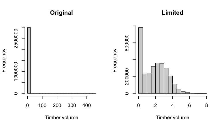
Resulting values at polygon geometries are rasterised with the workflow
egvtools::polygon2input(), restricting to pixels outside the clearcut mask. No
background values are assigned during rasterisation. The resulting layer is
then aggregated to EGV resolution using the workflow egvtools::input2egv() by calculating
sum of pixel values. After the aggregation, cells with no forest information
are filled with value 0. Finally, the layer is standardised by subtracting
the arithmetic mean and dividing by the root mean squared error.
Code
# libs ----
if(!require(egvtools)) {remotes::install_github("aavotins/egvtools"); require(egvtools)}
if(!require(terra)) {install.packages("terra"); require(terra)}
if(!require(sf)) {install.packages("sf"); require(sf)}
if(!require(tidyverse)) {install.packages("tidyverse"); require(tidyverse)}
if(!require(sfarrow)) {install.packages("sfarrow"); require(sfarrow)}
if(!require(readxl)) {install.packages("readxl"); require(readxl)}
if(!require(raster)) {install.packages("raster"); require(raster)}
if(!require(fasterize)) {install.packages("fasterize"); require(fasterize)}
# templates ----
template100=rast("./Templates/TemplateRasters/LV100m_10km.tif")
template10=rast("./Templates/TemplateRasters/LV10m_10km.tif")
rastrs10=raster(template10)
nulls10=rast("./Templates/TemplateRasters/nulls_LV10m_10km.tif")
nulls100=rast("./Templates/TemplateRasters/nulls_LV100m_10km.tif")
# simple landscape ----
simple_landscape=rast("RasterGrids_10m/2024/Ainava_vienk_mask.tif")
# mvr ----
mvr=st_read_parquet("./Geodata/2024/MVR/nogabali_2024janv.parquet")
mvr$yes=1
# clear cut mask ----
izcirtumi=mvr %>%
filter(zkat %in% c("12","14")) %>%
dplyr::select(yes)
r_izcirtumi_mvr=fasterize(izcirtumi,rastrs10,field="yes")
t_izcirtumi_mvr=rast(r_izcirtumi_mvr)
plot(t_izcirtumi_mvr)
tcl=rast("./Geodata/2024/Trees/GFW/TreeCoverLoss_v1_12.tif")
tcl2=ifel(tcl<20,0,1)
tclX=cover(tcl2,nulls10)
plot(tclX)
clearcut_mask=cover(t_izcirtumi_mvr,tclX,
filename="./RasterGrids_10m/2024/Mask_clearcuts.tif",
overwrite=TRUE)
plot(clearcut_mask)
rm(izcirtumi)
rm(r_izcirtumi_mvr)
rm(t_izcirtumi_mvr)
rm(tcl)
rm(tcl2)
rm(tclX)
# ForestsQuant_VolumeTotal-sum_cell.tif egv_307 ----
nogabali=mvr %>%
mutate(KopejaKraja=v10+v11+v12+v13+v14) %>%
mutate(KopejaKraja2=KopejaKraja/10000*10*10) %>%
mutate(KopejaKraja3=ifelse(KopejaKraja2>8,8,KopejaKraja2)) %>%
filter(!is.na(KopejaKraja2))
par(mfrow=c(1,2))
options(scipen=999)
hist(nogabali$KopejaKraja2,main="Original",xlab="Timber volume")
hist(nogabali$KopejaKraja3,main="Limited",xlab="Timber volume")
par(mfrow=c(1,1))
options(scipen=0)
p2i_rez=polygon2input(vector_data=nogabali,
template_path = "./Templates/TemplateRasters/LV10m_10km.tif",
out_path = "./RasterGrids_10m/2024/",
file_name = "ForestsQuant_VolumeTotal.tif",
value_field = "KopejaKraja3",
fun="max",
prepare=FALSE,
restrict_to = clearcut_mask,
restrict_values = 0,
plot_result=TRUE,
overwrite=TRUE)
p2i_rez
i2e_rez=input2egv(input="./RasterGrids_10m/2024/ForestsQuant_VolumeTotal.tif",
egv_template = "./Templates/TemplateRasters/LV100m_10km.tif",
summary_function = "sum",
missing_job = "CoverOutput",
output_bg = "./Templates/TemplateRasters/nulls_LV100m_10km.tif",
outlocation = "./RasterGrids_100m/2024/RAW/",
outfilename = "ForestsQuant_VolumeTotal-sum_cell.tif",
layername = "egv_307",
plot_final=TRUE)
i2e_rez
rm(p2i_rez)
rm(nogabali)
rm(i2e_rez)
unlink("./RasterGrids_10m/2024/ForestsQuant_VolumeTotal.tif")
# standardisation ----
if(!require(terra)) {install.packages("terra"); require(terra)}
if(!require(tidyverse)) {install.packages("tidyverse"); require(tidyverse)}
nosaukums="ForestsQuant_VolumeTotal-sum_cell.tif"
ielasisanas_cels=paste0("./RasterGrids_100m/2024/RAW/",nosaukums)
saglabasanas_cels=paste0("./RasterGrids_100m/2024/Scaled/",nosaukums)
slanis=rast(ielasisanas_cels)
videjais=global(slanis,fun="mean",na.rm=TRUE)
centrets=slanis-videjais[,1]
standartnovirze=terra::global(centrets,fun="rms",na.rm=TRUE)
merogots=centrets/standartnovirze[,1]
writeRaster(merogots,
filename=saglabasanas_cels,
overwrite=TRUE)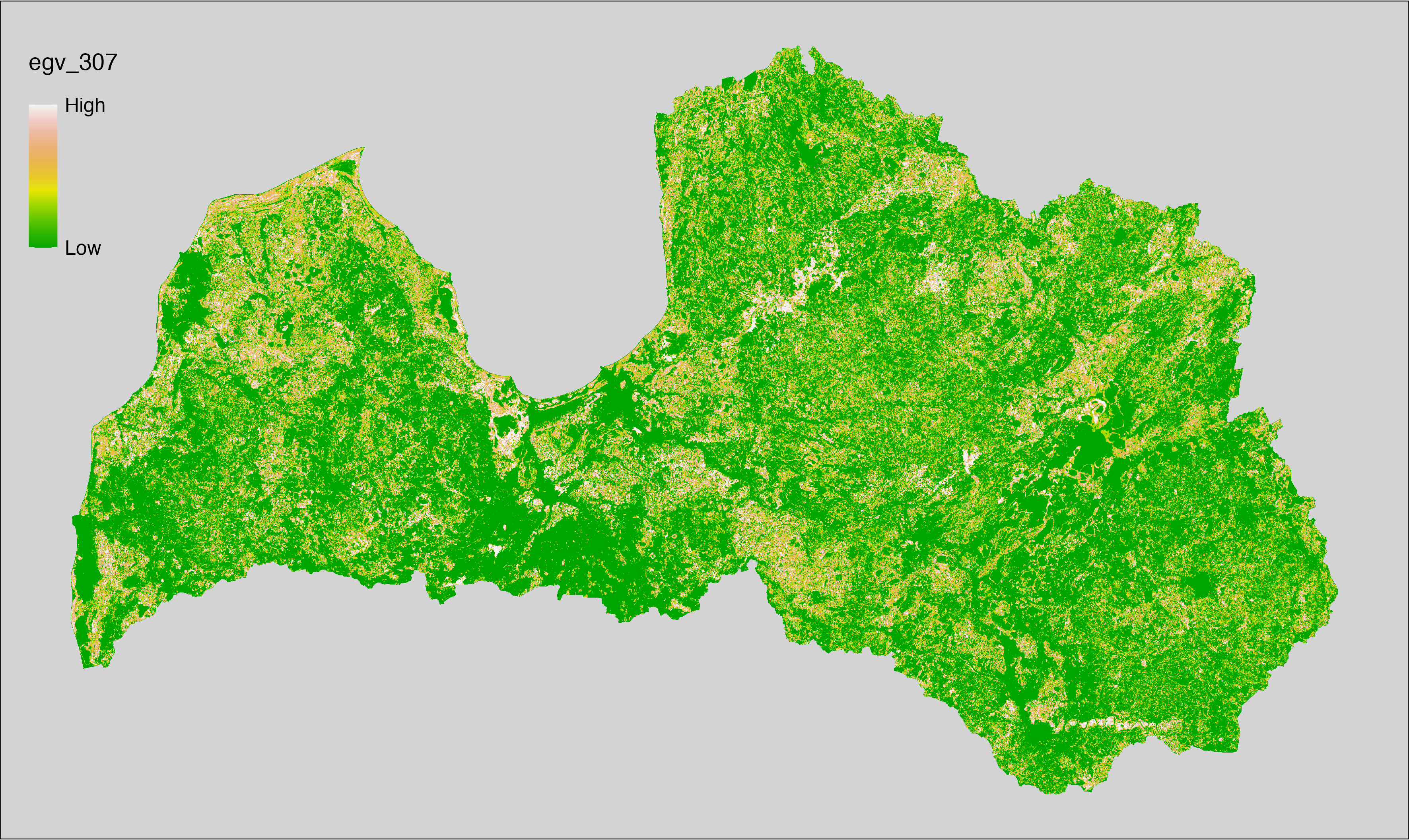
6.308 ForestsSoil_EutrophicDrained_cell
filename: ForestsSoil_EutrophicDrained_cell.tif
layername: egv_308
English name: Fractional cover of Drained Eutrophic Forests within the analysis cell (1 ha)
Latvian name: Susinātu eitrofu mežu platības īpatsvars analīzes šūnā (1 ha)
Procedure: To prepare this EGV, forest stands with forest type equal to
“19”, “21”, “24” or “25” are selected from the State Forest Service’s State Forest
Registry and rasterised. Rasterisation is performed using the
workflow egvtools::polygon2input() with background
covering (value 0). The resulting layer
is then aggregated to EGV resolution using the workflow egvtools::input2egv(), which
calculates the arithmetic mean to determine the cover fraction. During
aggregation, inverse distance weighted (power = 2) gap filling on the output is
applied to ensure no missing values at the edges. Finally, the layer is
standardised by subtracting the arithmetic mean and dividing by the root mean squared
error.
Code
# libs ----
if(!require(egvtools)) {remotes::install_github("aavotins/egvtools"); require(egvtools)}
if(!require(terra)) {install.packages("terra"); require(terra)}
if(!require(sf)) {install.packages("sf"); require(sf)}
if(!require(tidyverse)) {install.packages("tidyverse"); require(tidyverse)}
if(!require(sfarrow)) {install.packages("sfarrow"); require(sfarrow)}
if(!require(readxl)) {install.packages("readxl"); require(readxl)}
if(!require(raster)) {install.packages("raster"); require(raster)}
if(!require(fasterize)) {install.packages("fasterize"); require(fasterize)}
# templates ----
template100=rast("./Templates/TemplateRasters/LV100m_10km.tif")
template10=rast("./Templates/TemplateRasters/LV10m_10km.tif")
rastrs10=raster(template10)
nulls10=rast("./Templates/TemplateRasters/nulls_LV10m_10km.tif")
nulls100=rast("./Templates/TemplateRasters/nulls_LV100m_10km.tif")
# simple landscape ----
simple_landscape=rast("RasterGrids_10m/2024/Ainava_vienk_mask.tif")
# mvr ----
mvr=st_read_parquet("./Geodata/2024/MVR/nogabali_2024janv.parquet")
mvr$yes=1
# ForestsSoil_EutrophicDrained_cell.tif egv_308 ----
EutrophicDrained=mvr %>%
filter(mt %in% c("19","21","24","25"))
p2i_rez=egvtools::polygon2input(vector_data = EutrophicDrained,
template_path = "./Templates/TemplateRasters/LV10m_10km.tif",
out_path = "./RasterGrids_10m/2024/",
file_name = "ForestsSoil_EutrophicDrained_input.tif",
value_field = "yes",
prepare=FALSE,
background_raster = "./Templates/TemplateRasters/nulls_LV10m_10km.tif",
plot_result = TRUE)
p2i_rez
i2e_rez=egvtools::input2egv(input=paste0("./RasterGrids_10m/2024/",
"ForestsSoil_EutrophicDrained_input.tif"),
egv_template= "./Templates/TemplateRasters/LV100m_10km.tif",
summary_function = "average",
missing_job = "FillOutput",
outlocation = "./RasterGrids_100m/2024/RAW/",
outfilename = "ForestsSoil_EutrophicDrained_cell.tif",
layername = "egv_308",
idw_weight = 2,
plot_gaps = FALSE,plot_final = TRUE)
i2e_rez
rm(EutrophicDrained)
rm(p2i_rez)
rm(i2e_rez)
unlink("./RasterGrids_10m/2024/ForestsSoil_EutrophicDrained_input.tif")
# standardisation ----
if(!require(terra)) {install.packages("terra"); require(terra)}
if(!require(tidyverse)) {install.packages("tidyverse"); require(tidyverse)}
nosaukums="ForestsSoil_EutrophicDrained_cell.tif"
ielasisanas_cels=paste0("./RasterGrids_100m/2024/RAW/",nosaukums)
saglabasanas_cels=paste0("./RasterGrids_100m/2024/Scaled/",nosaukums)
slanis=rast(ielasisanas_cels)
videjais=global(slanis,fun="mean",na.rm=TRUE)
centrets=slanis-videjais[,1]
standartnovirze=terra::global(centrets,fun="rms",na.rm=TRUE)
merogots=centrets/standartnovirze[,1]
writeRaster(merogots,
filename=saglabasanas_cels,
overwrite=TRUE)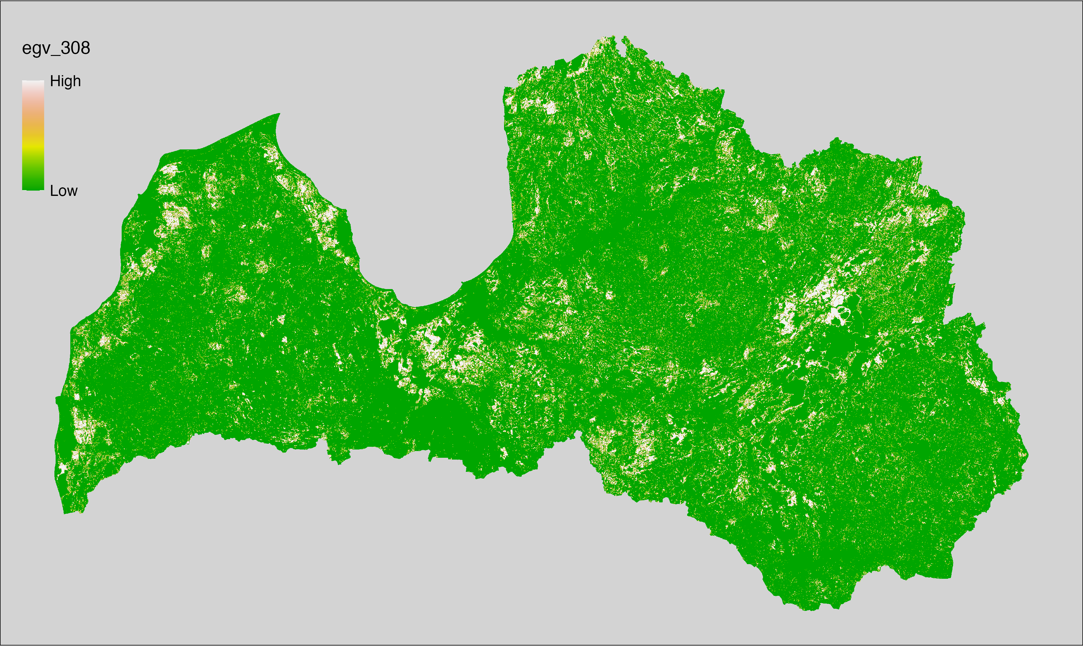
6.309 ForestsSoil_EutrophicDrained_r500
filename: ForestsSoil_EutrophicDrained_r500.tif
layername: egv_309
English name: Fractional cover of Drained Eutrophic Forests within the 0.5 km landscape
Latvian name: Susinātu eitrofu mežu platības īpatsvars 0,5 km ainavā
Procedure: The cover fraction within a radius of 500 m around the analysis grid cell is
calculated as the area-weighted sum of the analysis cells inside the
buffer, using the workflow egvtools::radius_function(). During the calculation of the landscape metric,
inverse distance weighted (power = 2) gap filling on the output is applied
to ensure no missing values at the edges. Then the layer is rewritten to set
its name. Finally, the layer is standardised by subtracting the arithmetic
mean and dividing by the root mean squared error.
Code
# libs ----
if(!require(terra)) {install.packages("terra"); require(terra)}
if(!require(egvtools)) {remotes::install_github("aavotins/egvtools"); require(egvtools)}
# Templates -----
template100=rast("./Templates/TemplateRasters/LV100m_10km.tif")
# radii ----
radius_function(
kvadrati_path = "./Templates/TemplateGrids/tiles/",
radii_path = "./Templates/TemplateGridPoints/tiles/",
tikls100_path = "./Templates/TemplateGrids/tikls100_sauzeme.parquet",
template_path = "./Templates/TemplateRasters/LV100m_10km.tif",
input_layers = c("./RasterGrids_100m/2024/RAW/ForestsSoil_EutrophicDrained_cell.tif"),
layer_prefixes = c("ForestsSoil_EutrophicDrained"),
output_dir = "./RasterGrids_100m/2024/RAW/",
n_workers = 6,
radii = c("r500"),
radius_mode = "sparse",
extract_fun = "mean",
fill_missing = TRUE,
IDW_weight = 2,
future_max_size = 40 * 1024^3)
# ForestsSoil_EutrophicDrained_r500.tif egv_309
slanis=rast("./RasterGrids_100m/2024/RAW/ForestsSoil_EutrophicDrained_r500.tif")
names(slanis)="egv_309"
slanis2=project(slanis,template100)
writeRaster(slanis2,
"./RasterGrids_100m/2024/RAW/ForestsSoil_EutrophicDrained_r500.tif",
overwrite=TRUE)
# standardisation ----
if(!require(terra)) {install.packages("terra"); require(terra)}
if(!require(tidyverse)) {install.packages("tidyverse"); require(tidyverse)}
nosaukums="ForestsSoil_EutrophicDrained_r500.tif"
ielasisanas_cels=paste0("./RasterGrids_100m/2024/RAW/",nosaukums)
saglabasanas_cels=paste0("./RasterGrids_100m/2024/Scaled/",nosaukums)
slanis=rast(ielasisanas_cels)
videjais=global(slanis,fun="mean",na.rm=TRUE)
centrets=slanis-videjais[,1]
standartnovirze=terra::global(centrets,fun="rms",na.rm=TRUE)
merogots=centrets/standartnovirze[,1]
writeRaster(merogots,
filename=saglabasanas_cels,
overwrite=TRUE)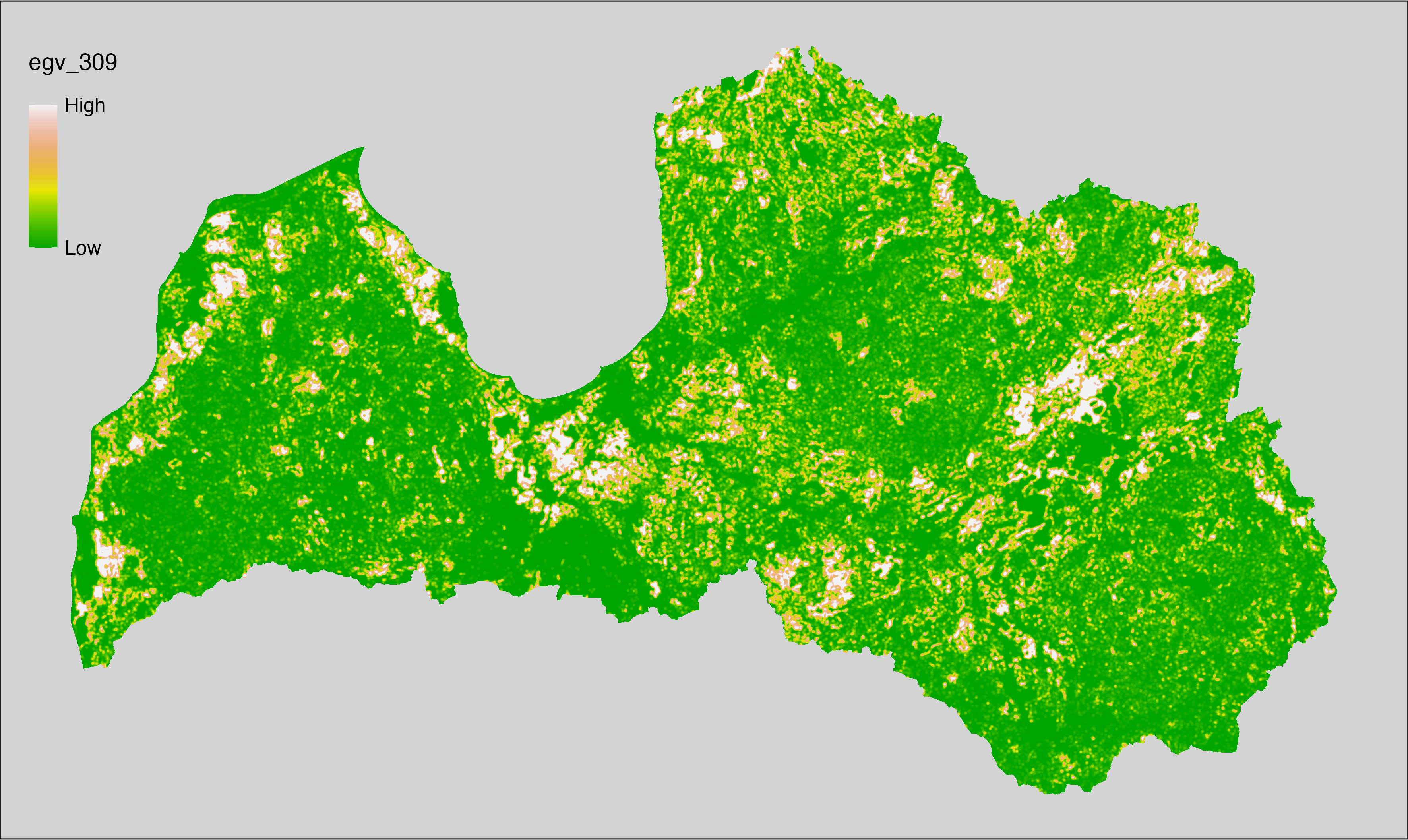
6.310 ForestsSoil_EutrophicDrained_r1250
filename: ForestsSoil_EutrophicDrained_r1250.tif
layername: egv_310
English name: Fractional cover of Drained Eutrophic Forests within the 1.25 km landscape
Latvian name: Susinātu eitrofu mežu platības īpatsvars 1,25 km ainavā
Procedure: The cover fraction within a radius of 1250 m around the analysis grid cell
is calculated as the area-weighted sum of the analysis cells inside
the buffer, using the workflow egvtools::radius_function(). During the calculation of the landscape
metric, inverse distance weighted (power = 2) gap filling on the output is
applied to ensure no missing values at the edges. Then the layer is
rewritten to set its name. Finally, the layer is standardised by
subtracting the arithmetic mean and dividing by the root mean squared error.
Code
# libs ----
if(!require(terra)) {install.packages("terra"); require(terra)}
if(!require(egvtools)) {remotes::install_github("aavotins/egvtools"); require(egvtools)}
# Templates -----
template100=rast("./Templates/TemplateRasters/LV100m_10km.tif")
# radii ----
radius_function(
kvadrati_path = "./Templates/TemplateGrids/tiles/",
radii_path = "./Templates/TemplateGridPoints/tiles/",
tikls100_path = "./Templates/TemplateGrids/tikls100_sauzeme.parquet",
template_path = "./Templates/TemplateRasters/LV100m_10km.tif",
input_layers = c("./RasterGrids_100m/2024/RAW/ForestsSoil_EutrophicDrained_cell.tif"),
layer_prefixes = c("ForestsSoil_EutrophicDrained"),
output_dir = "./RasterGrids_100m/2024/RAW/",
n_workers = 6,
radii = c("r1250"),
radius_mode = "sparse",
extract_fun = "mean",
fill_missing = TRUE,
IDW_weight = 2,
future_max_size = 40 * 1024^3)
# ForestsSoil_EutrophicDrained_r1250.tif egv_310
slanis=rast("./RasterGrids_100m/2024/RAW/ForestsSoil_EutrophicDrained_r1250.tif")
names(slanis)="egv_310"
slanis2=project(slanis,template100)
writeRaster(slanis2,
"./RasterGrids_100m/2024/RAW/ForestsSoil_EutrophicDrained_r1250.tif",
overwrite=TRUE)
# standardisation ----
if(!require(terra)) {install.packages("terra"); require(terra)}
if(!require(tidyverse)) {install.packages("tidyverse"); require(tidyverse)}
nosaukums="ForestsSoil_EutrophicDrained_r1250.tif"
ielasisanas_cels=paste0("./RasterGrids_100m/2024/RAW/",nosaukums)
saglabasanas_cels=paste0("./RasterGrids_100m/2024/Scaled/",nosaukums)
slanis=rast(ielasisanas_cels)
videjais=global(slanis,fun="mean",na.rm=TRUE)
centrets=slanis-videjais[,1]
standartnovirze=terra::global(centrets,fun="rms",na.rm=TRUE)
merogots=centrets/standartnovirze[,1]
writeRaster(merogots,
filename=saglabasanas_cels,
overwrite=TRUE)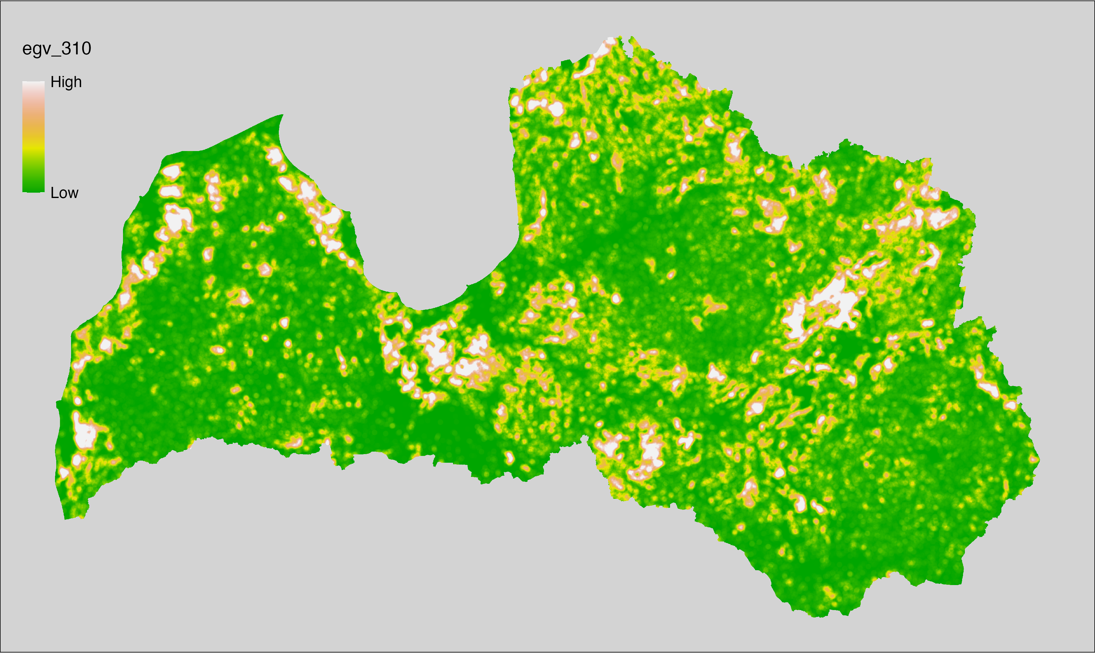
6.311 ForestsSoil_EutrophicDrained_r3000
filename: ForestsSoil_EutrophicDrained_r3000.tif
layername: egv_311
English name: Fractional cover of Drained Eutrophic Forests within the 3 km landscape
Latvian name: Susinātu eitrofu mežu platības īpatsvars 3 km ainavā
Procedure: The cover fraction within a radius of 3000 m around the analysis grid cell
is calculated as the area-weighted sum of the analysis cells inside
the buffer, using the workflow egvtools::radius_function(). During the calculation of the landscape
metric, inverse distance weighted (power = 2) gap filling on the output is
applied to ensure no missing values at the edges. Then the layer is
rewritten to set its name. Finally, the layer is standardised by
subtracting the arithmetic mean and dividing by the root mean squared error.
Code
# libs ----
if(!require(terra)) {install.packages("terra"); require(terra)}
if(!require(egvtools)) {remotes::install_github("aavotins/egvtools"); require(egvtools)}
# Templates -----
template100=rast("./Templates/TemplateRasters/LV100m_10km.tif")
# radii ----
radius_function(
kvadrati_path = "./Templates/TemplateGrids/tiles/",
radii_path = "./Templates/TemplateGridPoints/tiles/",
tikls100_path = "./Templates/TemplateGrids/tikls100_sauzeme.parquet",
template_path = "./Templates/TemplateRasters/LV100m_10km.tif",
input_layers = c("./RasterGrids_100m/2024/RAW/ForestsSoil_EutrophicDrained_cell.tif"),
layer_prefixes = c("ForestsSoil_EutrophicDrained"),
output_dir = "./RasterGrids_100m/2024/RAW/",
n_workers = 6,
radii = c("r3000"),
radius_mode = "sparse",
extract_fun = "mean",
fill_missing = TRUE,
IDW_weight = 2,
future_max_size = 40 * 1024^3)
# ForestsSoil_EutrophicDrained_r3000.tif egv_311
slanis=rast("./RasterGrids_100m/2024/RAW/ForestsSoil_EutrophicDrained_r3000.tif")
names(slanis)="egv_311"
slanis2=project(slanis,template100)
writeRaster(slanis2,
"./RasterGrids_100m/2024/RAW/ForestsSoil_EutrophicDrained_r3000.tif",
overwrite=TRUE)
# standardisation ----
if(!require(terra)) {install.packages("terra"); require(terra)}
if(!require(tidyverse)) {install.packages("tidyverse"); require(tidyverse)}
nosaukums="ForestsSoil_EutrophicDrained_r3000.tif"
ielasisanas_cels=paste0("./RasterGrids_100m/2024/RAW/",nosaukums)
saglabasanas_cels=paste0("./RasterGrids_100m/2024/Scaled/",nosaukums)
slanis=rast(ielasisanas_cels)
videjais=global(slanis,fun="mean",na.rm=TRUE)
centrets=slanis-videjais[,1]
standartnovirze=terra::global(centrets,fun="rms",na.rm=TRUE)
merogots=centrets/standartnovirze[,1]
writeRaster(merogots,
filename=saglabasanas_cels,
overwrite=TRUE)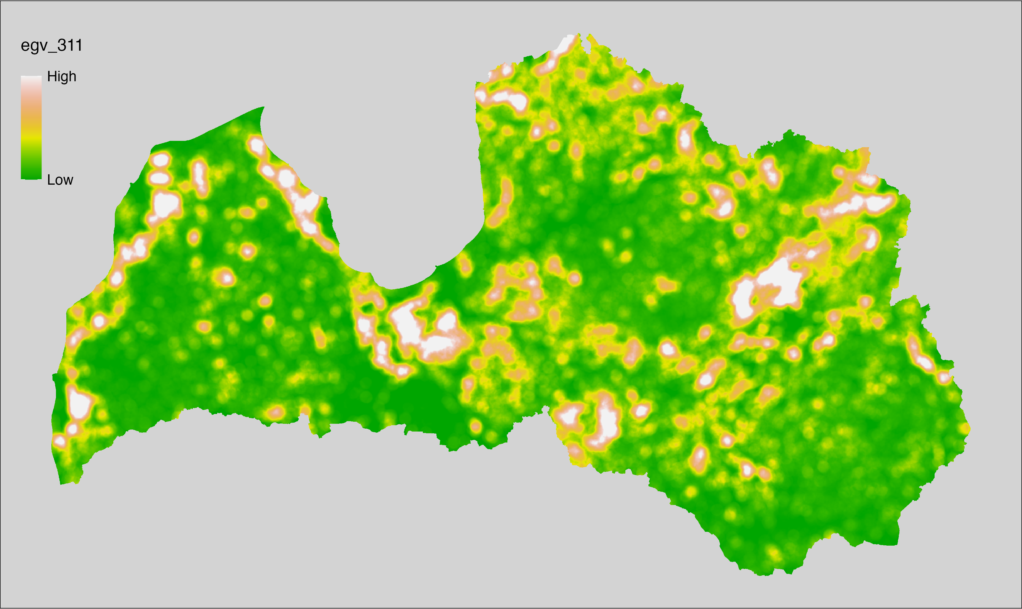
6.312 ForestsSoil_EutrophicDrained_r10000
filename: ForestsSoil_EutrophicDrained_r10000.tif
layername: egv_312
English name: Fractional cover of Drained Eutrophic Forests within the 10 km landscape
Latvian name: Susinātu eitrofu mežu platības īpatsvars 10 km ainavā
Procedure: The cover fraction within a radius of 10000 m around the analysis grid cell
is calculated as the area-weighted sum of the analysis cells inside
the buffer, using the workflow egvtools::radius_function(). During the calculation of the landscape
metric, inverse distance weighted (power = 2) gap filling on the output is
applied to ensure no missing values at the edges. Then the layer is
rewritten to set its name. Finally, the layer is standardised by
subtracting the arithmetic mean and dividing by the root mean squared error.
Code
# libs ----
if(!require(terra)) {install.packages("terra"); require(terra)}
if(!require(egvtools)) {remotes::install_github("aavotins/egvtools"); require(egvtools)}
# Templates -----
template100=rast("./Templates/TemplateRasters/LV100m_10km.tif")
# radii ----
radius_function(
kvadrati_path = "./Templates/TemplateGrids/tiles/",
radii_path = "./Templates/TemplateGridPoints/tiles/",
tikls100_path = "./Templates/TemplateGrids/tikls100_sauzeme.parquet",
template_path = "./Templates/TemplateRasters/LV100m_10km.tif",
input_layers = c("./RasterGrids_100m/2024/RAW/ForestsSoil_EutrophicDrained_cell.tif"),
layer_prefixes = c("ForestsSoil_EutrophicDrained"),
output_dir = "./RasterGrids_100m/2024/RAW/",
n_workers = 6,
radii = c("r10000"),
radius_mode = "sparse",
extract_fun = "mean",
fill_missing = TRUE,
IDW_weight = 2,
future_max_size = 40 * 1024^3)
# ForestsSoil_EutrophicDrained_r10000.tif egv_312
slanis=rast("./RasterGrids_100m/2024/RAW/ForestsSoil_EutrophicDrained_r10000.tif")
names(slanis)="egv_312"
slanis2=project(slanis,template100)
writeRaster(slanis2,
"./RasterGrids_100m/2024/RAW/ForestsSoil_EutrophicDrained_r10000.tif",
overwrite=TRUE)
# standardisation ----
if(!require(terra)) {install.packages("terra"); require(terra)}
if(!require(tidyverse)) {install.packages("tidyverse"); require(tidyverse)}
nosaukums="ForestsSoil_EutrophicDrained_r10000.tif"
ielasisanas_cels=paste0("./RasterGrids_100m/2024/RAW/",nosaukums)
saglabasanas_cels=paste0("./RasterGrids_100m/2024/Scaled/",nosaukums)
slanis=rast(ielasisanas_cels)
videjais=global(slanis,fun="mean",na.rm=TRUE)
centrets=slanis-videjais[,1]
standartnovirze=terra::global(centrets,fun="rms",na.rm=TRUE)
merogots=centrets/standartnovirze[,1]
writeRaster(merogots,
filename=saglabasanas_cels,
overwrite=TRUE)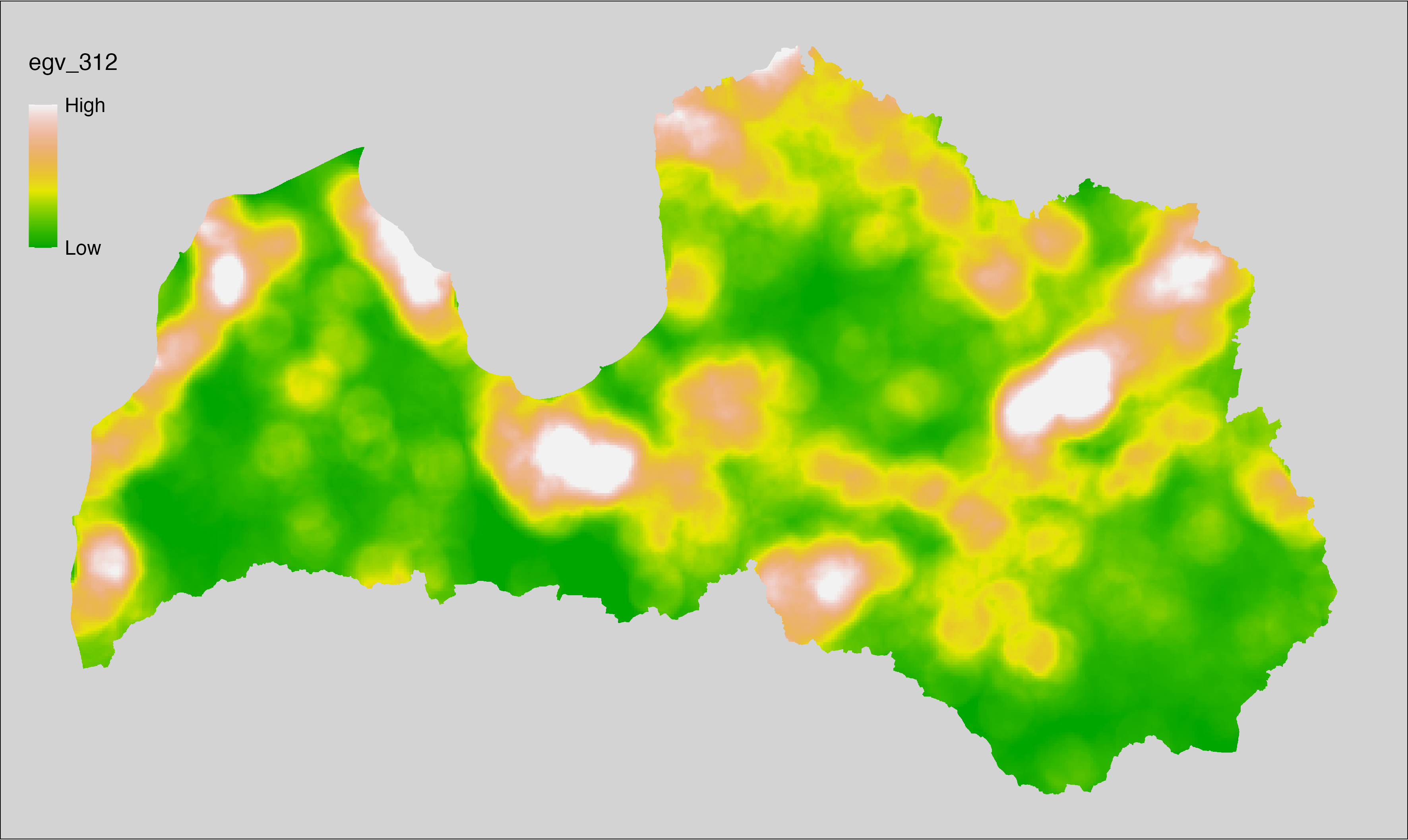
6.313 ForestsSoil_EutrophicMineral_cell
filename: ForestsSoil_EutrophicMineral_cell.tif
layername: egv_313
English name: Fractional cover of Eutrophic Forests on undrained Mineral Soils within the analysis cell (1 ha)
Latvian name: Eitrofu mežu nesusinātās minerālaugsnēs platības īpatsvars analīzes šūnā (1 ha)
Procedure: To prepare this EGV, forest stands with forest type equal to “5”,
“6”, “10” or “11” are selected from the State Forest Service’s State Forest
Registry and rasterised. Rasterisation is performed using
the workflow egvtools::polygon2input() with background
covering (value 0). The resulting layer
is then aggregated to EGV resolution using the workflow egvtools::input2egv(), which
calculates the arithmetic mean to determine the cover fraction. During
aggregation, inverse distance weighted (power = 2) gap filling on the output is
applied to ensure no missing values at the edges. Finally, the layer is
standardised by subtracting the arithmetic mean and dividing by the root mean squared
error.
Code
# libs ----
if(!require(egvtools)) {remotes::install_github("aavotins/egvtools"); require(egvtools)}
if(!require(terra)) {install.packages("terra"); require(terra)}
if(!require(sf)) {install.packages("sf"); require(sf)}
if(!require(tidyverse)) {install.packages("tidyverse"); require(tidyverse)}
if(!require(sfarrow)) {install.packages("sfarrow"); require(sfarrow)}
if(!require(readxl)) {install.packages("readxl"); require(readxl)}
if(!require(raster)) {install.packages("raster"); require(raster)}
if(!require(fasterize)) {install.packages("fasterize"); require(fasterize)}
# templates ----
template100=rast("./Templates/TemplateRasters/LV100m_10km.tif")
template10=rast("./Templates/TemplateRasters/LV10m_10km.tif")
rastrs10=raster(template10)
nulls10=rast("./Templates/TemplateRasters/nulls_LV10m_10km.tif")
nulls100=rast("./Templates/TemplateRasters/nulls_LV100m_10km.tif")
# simple landscape ----
simple_landscape=rast("RasterGrids_10m/2024/Ainava_vienk_mask.tif")
# mvr ----
mvr=st_read_parquet("./Geodata/2024/MVR/nogabali_2024janv.parquet")
mvr$yes=1
# ForestsSoil_EutrophicMineral_cell.tif egv_313 ----
EutrophicMineral=mvr %>%
filter(mt %in% c("5","6","10","11"))
p2i_rez=egvtools::polygon2input(vector_data = EutrophicMineral,
template_path = "./Templates/TemplateRasters/LV10m_10km.tif",
out_path = "./RasterGrids_10m/2024/",
file_name = "ForestsSoil_EutrophicMineral_input.tif",
value_field = "yes",
prepare=FALSE,
background_raster = "./Templates/TemplateRasters/nulls_LV10m_10km.tif",
plot_result = TRUE)
p2i_rez
i2e_rez=egvtools::input2egv(input=paste0("./RasterGrids_10m/2024/",
"ForestsSoil_EutrophicMineral_input.tif"),
egv_template= "./Templates/TemplateRasters/LV100m_10km.tif",
summary_function = "average",
missing_job = "FillOutput",
outlocation = "./RasterGrids_100m/2024/RAW/",
outfilename = "ForestsSoil_EutrophicMineral_cell.tif",
layername = "egv_313",
idw_weight = 2,
plot_gaps = FALSE,plot_final = TRUE)
i2e_rez
rm(EutrophicMineral)
rm(p2i_rez)
rm(i2e_rez)
unlink("./RasterGrids_10m/2024/ForestsSoil_EutrophicMineral_input.tif")
# standardisation ----
if(!require(terra)) {install.packages("terra"); require(terra)}
if(!require(tidyverse)) {install.packages("tidyverse"); require(tidyverse)}
nosaukums="ForestsSoil_EutrophicMineral_cell.tif"
ielasisanas_cels=paste0("./RasterGrids_100m/2024/RAW/",nosaukums)
saglabasanas_cels=paste0("./RasterGrids_100m/2024/Scaled/",nosaukums)
slanis=rast(ielasisanas_cels)
videjais=global(slanis,fun="mean",na.rm=TRUE)
centrets=slanis-videjais[,1]
standartnovirze=terra::global(centrets,fun="rms",na.rm=TRUE)
merogots=centrets/standartnovirze[,1]
writeRaster(merogots,
filename=saglabasanas_cels,
overwrite=TRUE)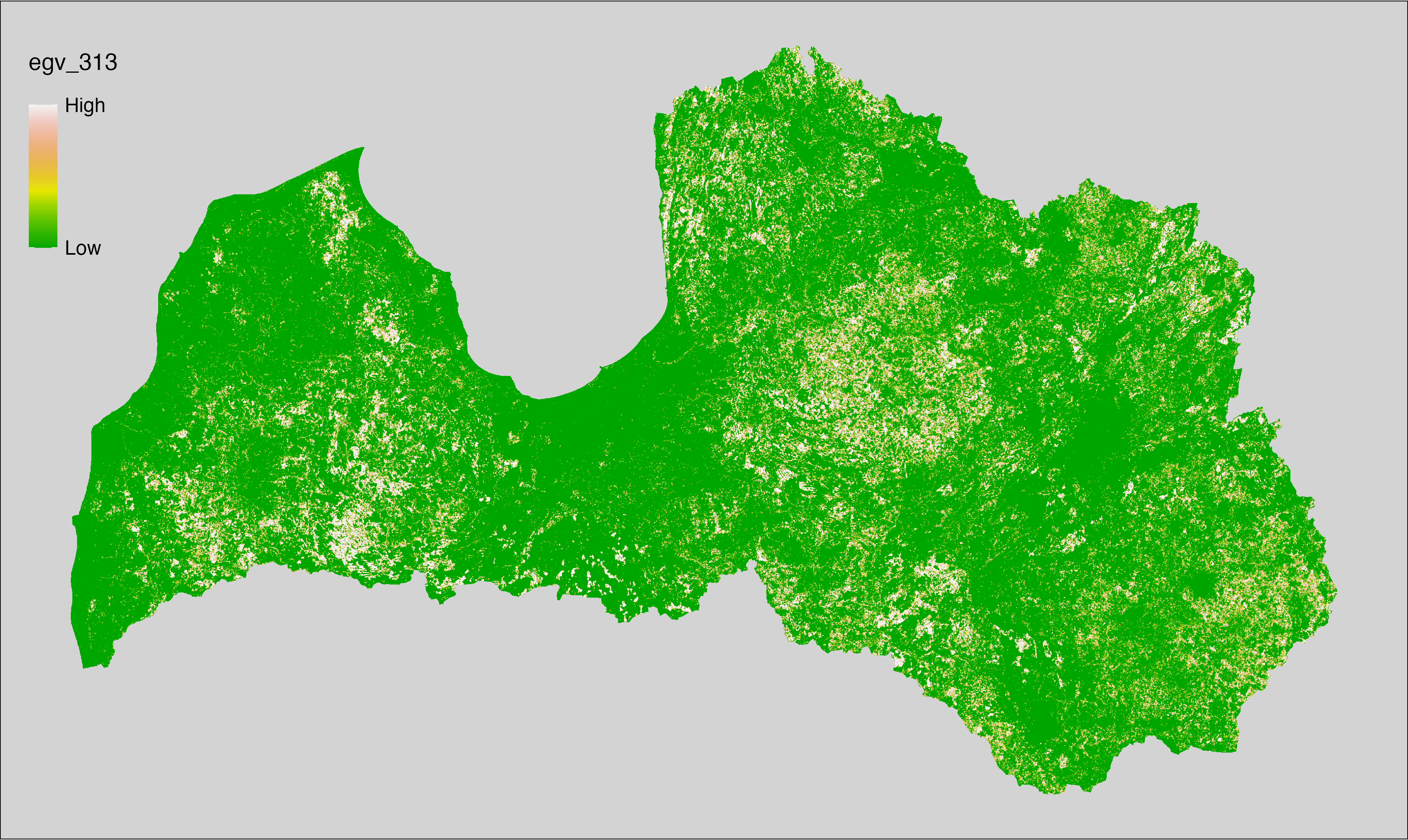
6.314 ForestsSoil_EutrophicMineral_r500
filename: ForestsSoil_EutrophicMineral_r500.tif
layername: egv_314
English name: Fractional cover of Eutrophic Forests on undrained Mineral Soils within the 0.5 km landscape
Latvian name: Eitrofu mežu nesusinātās minerālaugsnēs platības īpatsvars 0,5 km ainavā
Procedure: The cover fraction within a radius of 500 m around the analysis grid cell is
calculated as the area-weighted sum of the analysis cells inside the
buffer, using the workflow egvtools::radius_function(). During the calculation of the landscape metric,
inverse distance weighted (power = 2) gap filling on the output is applied
to ensure no missing values at the edges. Then the layer is rewritten to set
its name. Finally, the layer is standardised by subtracting the arithmetic
mean and dividing by the root mean squared error.
Code
# libs ----
if(!require(terra)) {install.packages("terra"); require(terra)}
if(!require(egvtools)) {remotes::install_github("aavotins/egvtools"); require(egvtools)}
# Templates -----
template100=rast("./Templates/TemplateRasters/LV100m_10km.tif")
# radii ----
radius_function(
kvadrati_path = "./Templates/TemplateGrids/tiles/",
radii_path = "./Templates/TemplateGridPoints/tiles/",
tikls100_path = "./Templates/TemplateGrids/tikls100_sauzeme.parquet",
template_path = "./Templates/TemplateRasters/LV100m_10km.tif",
input_layers = c("./RasterGrids_100m/2024/RAW/ForestsSoil_EutrophicMineral_cell.tif"),
layer_prefixes = c("ForestsSoil_EutrophicMineral"),
output_dir = "./RasterGrids_100m/2024/RAW/",
n_workers = 6,
radii = c("r500"),
radius_mode = "sparse",
extract_fun = "mean",
fill_missing = TRUE,
IDW_weight = 2,
future_max_size = 40 * 1024^3)
# ForestsSoil_EutrophicMineral_r500.tif egv_314
slanis=rast("./RasterGrids_100m/2024/RAW/ForestsSoil_EutrophicMineral_r500.tif")
names(slanis)="egv_314"
slanis2=project(slanis,template100)
writeRaster(slanis2,
"./RasterGrids_100m/2024/RAW/ForestsSoil_EutrophicMineral_r500.tif",
overwrite=TRUE)
# standardisation ----
if(!require(terra)) {install.packages("terra"); require(terra)}
if(!require(tidyverse)) {install.packages("tidyverse"); require(tidyverse)}
nosaukums="ForestsSoil_EutrophicMineral_r500.tif"
ielasisanas_cels=paste0("./RasterGrids_100m/2024/RAW/",nosaukums)
saglabasanas_cels=paste0("./RasterGrids_100m/2024/Scaled/",nosaukums)
slanis=rast(ielasisanas_cels)
videjais=global(slanis,fun="mean",na.rm=TRUE)
centrets=slanis-videjais[,1]
standartnovirze=terra::global(centrets,fun="rms",na.rm=TRUE)
merogots=centrets/standartnovirze[,1]
writeRaster(merogots,
filename=saglabasanas_cels,
overwrite=TRUE)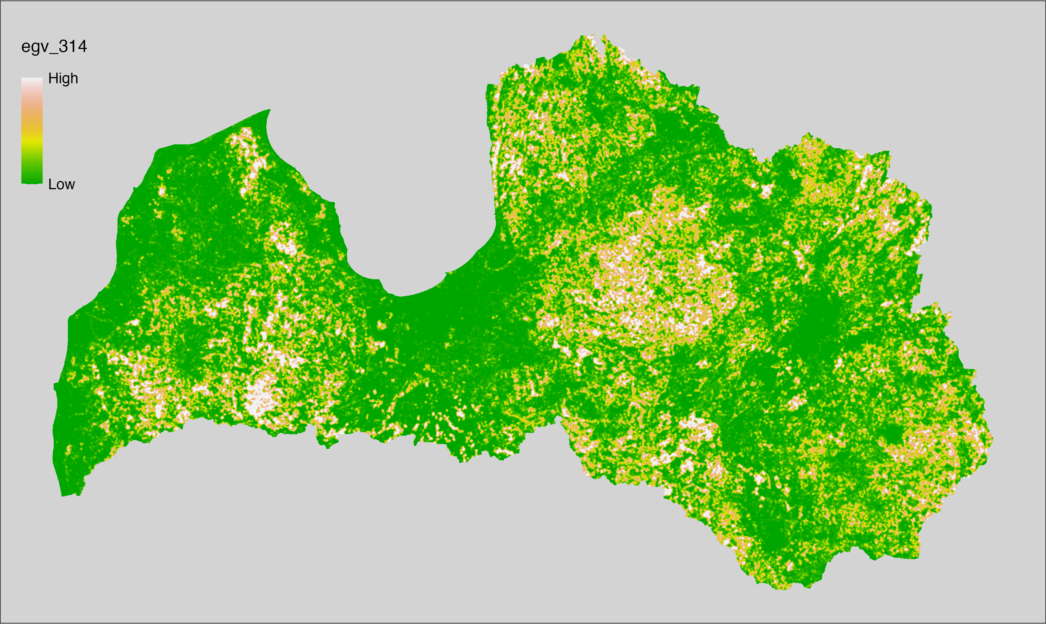
6.315 ForestsSoil_EutrophicMineral_r1250
filename: ForestsSoil_EutrophicMineral_r1250.tif
layername: egv_315
English name: Fractional cover of Eutrophic Forests on undrained Mineral Soils within the 1.25 km landscape
Latvian name: Eitrofu mežu nesusinātās minerālaugsnēs platības īpatsvars 1,25 km ainavā
Procedure: The cover fraction within a radius of 1250 m around the analysis grid cell
is calculated as the area-weighted sum of the analysis cells inside
the buffer, using the workflow egvtools::radius_function(). During the calculation of the landscape
metric, inverse distance weighted (power = 2) gap filling on the output is
applied to ensure no missing values at the edges. Then the layer is
rewritten to set its name. Finally, the layer is standardised by
subtracting the arithmetic mean and dividing by the root mean squared error.
Code
# libs ----
if(!require(terra)) {install.packages("terra"); require(terra)}
if(!require(egvtools)) {remotes::install_github("aavotins/egvtools"); require(egvtools)}
# Templates -----
template100=rast("./Templates/TemplateRasters/LV100m_10km.tif")
# radii ----
radius_function(
kvadrati_path = "./Templates/TemplateGrids/tiles/",
radii_path = "./Templates/TemplateGridPoints/tiles/",
tikls100_path = "./Templates/TemplateGrids/tikls100_sauzeme.parquet",
template_path = "./Templates/TemplateRasters/LV100m_10km.tif",
input_layers = c("./RasterGrids_100m/2024/RAW/ForestsSoil_EutrophicMineral_cell.tif"),
layer_prefixes = c("ForestsSoil_EutrophicMineral"),
output_dir = "./RasterGrids_100m/2024/RAW/",
n_workers = 6,
radii = c("r1250"),
radius_mode = "sparse",
extract_fun = "mean",
fill_missing = TRUE,
IDW_weight = 2,
future_max_size = 40 * 1024^3)
# ForestsSoil_EutrophicMineral_r1250.tif egv_315
slanis=rast("./RasterGrids_100m/2024/RAW/ForestsSoil_EutrophicMineral_r1250.tif")
names(slanis)="egv_315"
slanis2=project(slanis,template100)
writeRaster(slanis2,
"./RasterGrids_100m/2024/RAW/ForestsSoil_EutrophicMineral_r1250.tif",
overwrite=TRUE)
# standardisation ----
if(!require(terra)) {install.packages("terra"); require(terra)}
if(!require(tidyverse)) {install.packages("tidyverse"); require(tidyverse)}
nosaukums="ForestsSoil_EutrophicMineral_r1250.tif"
ielasisanas_cels=paste0("./RasterGrids_100m/2024/RAW/",nosaukums)
saglabasanas_cels=paste0("./RasterGrids_100m/2024/Scaled/",nosaukums)
slanis=rast(ielasisanas_cels)
videjais=global(slanis,fun="mean",na.rm=TRUE)
centrets=slanis-videjais[,1]
standartnovirze=terra::global(centrets,fun="rms",na.rm=TRUE)
merogots=centrets/standartnovirze[,1]
writeRaster(merogots,
filename=saglabasanas_cels,
overwrite=TRUE)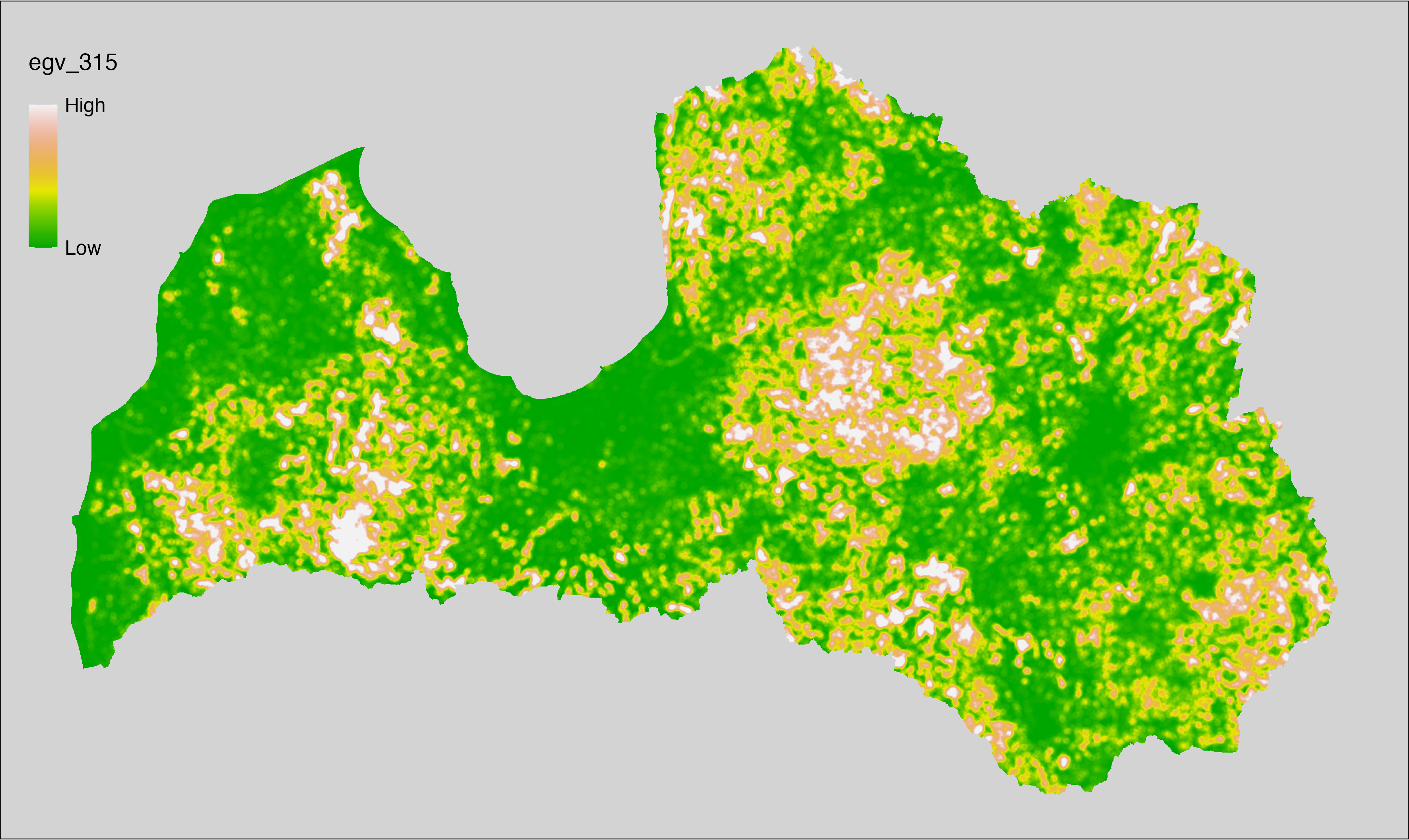
6.316 ForestsSoil_EutrophicMineral_r3000
filename: ForestsSoil_EutrophicMineral_r3000.tif
layername: egv_316
English name: Fractional cover of Eutrophic Forests on undrained Mineral Soils within the 3 km landscape
Latvian name: Eitrofu mežu nesusinātās minerālaugsnēs platības īpatsvars 3 km ainavā
Procedure: The cover fraction within a radius of 3000 m around the analysis grid cell
is calculated as the area-weighted sum of the analysis cells inside
the buffer, using the workflow egvtools::radius_function(). During the calculation of the landscape
metric, inverse distance weighted (power = 2) gap filling on the output is
applied to ensure no missing values at the edges. Then the layer is
rewritten to set its name. Finally, the layer is standardised by
subtracting the arithmetic mean and dividing by the root mean squared error.
Code
# libs ----
if(!require(terra)) {install.packages("terra"); require(terra)}
if(!require(egvtools)) {remotes::install_github("aavotins/egvtools"); require(egvtools)}
# Templates -----
template100=rast("./Templates/TemplateRasters/LV100m_10km.tif")
# radii ----
radius_function(
kvadrati_path = "./Templates/TemplateGrids/tiles/",
radii_path = "./Templates/TemplateGridPoints/tiles/",
tikls100_path = "./Templates/TemplateGrids/tikls100_sauzeme.parquet",
template_path = "./Templates/TemplateRasters/LV100m_10km.tif",
input_layers = c("./RasterGrids_100m/2024/RAW/ForestsSoil_EutrophicMineral_cell.tif"),
layer_prefixes = c("ForestsSoil_EutrophicMineral"),
output_dir = "./RasterGrids_100m/2024/RAW/",
n_workers = 6,
radii = c("r3000"),
radius_mode = "sparse",
extract_fun = "mean",
fill_missing = TRUE,
IDW_weight = 2,
future_max_size = 40 * 1024^3)
# ForestsSoil_EutrophicMineral_r3000.tif egv_316
slanis=rast("./RasterGrids_100m/2024/RAW/ForestsSoil_EutrophicMineral_r3000.tif")
names(slanis)="egv_316"
slanis2=project(slanis,template100)
writeRaster(slanis2,
"./RasterGrids_100m/2024/RAW/ForestsSoil_EutrophicMineral_r3000.tif",
overwrite=TRUE)
# standardisation ----
if(!require(terra)) {install.packages("terra"); require(terra)}
if(!require(tidyverse)) {install.packages("tidyverse"); require(tidyverse)}
nosaukums="ForestsSoil_EutrophicMineral_r3000.tif"
ielasisanas_cels=paste0("./RasterGrids_100m/2024/RAW/",nosaukums)
saglabasanas_cels=paste0("./RasterGrids_100m/2024/Scaled/",nosaukums)
slanis=rast(ielasisanas_cels)
videjais=global(slanis,fun="mean",na.rm=TRUE)
centrets=slanis-videjais[,1]
standartnovirze=terra::global(centrets,fun="rms",na.rm=TRUE)
merogots=centrets/standartnovirze[,1]
writeRaster(merogots,
filename=saglabasanas_cels,
overwrite=TRUE)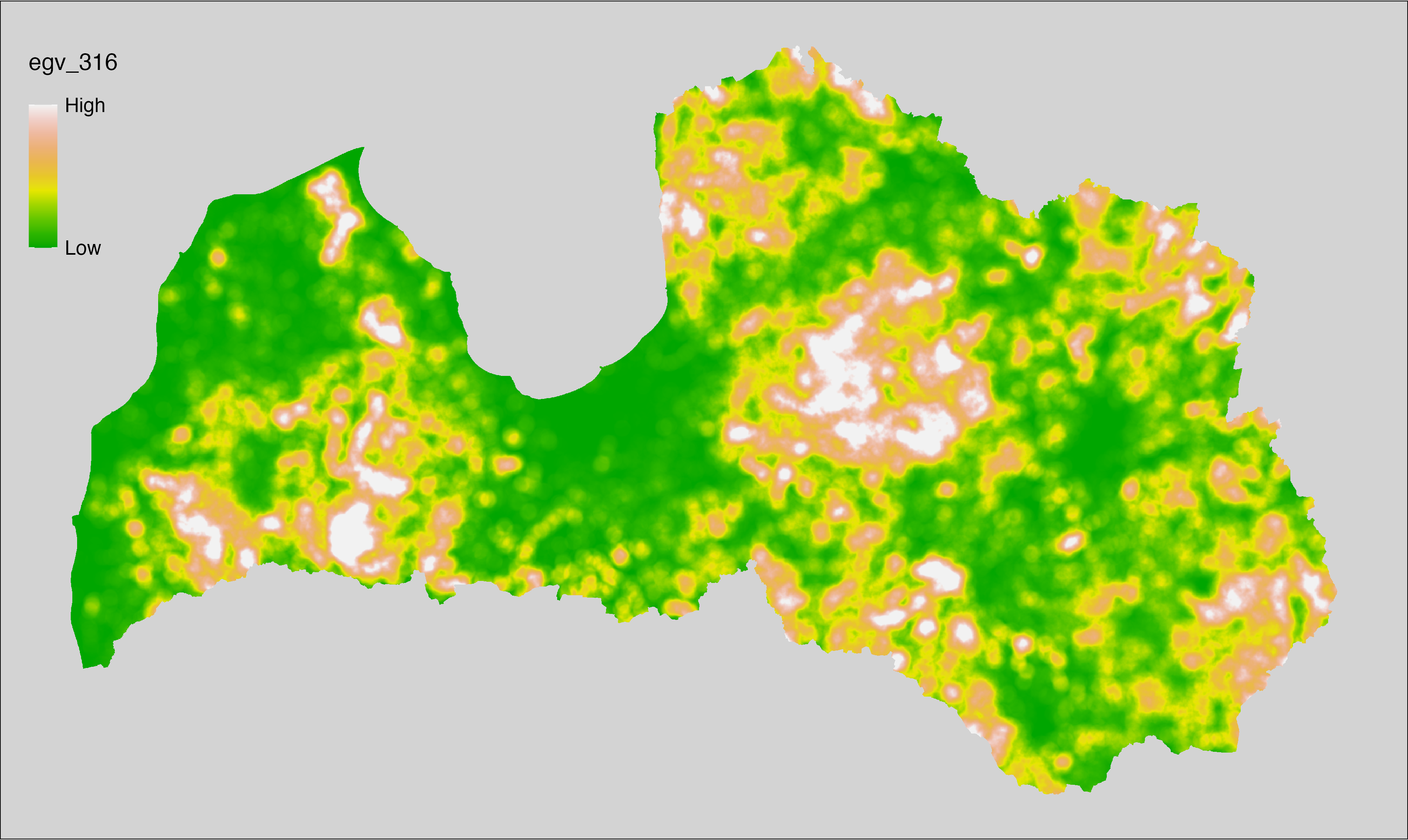
6.317 ForestsSoil_EutrophicMineral_r10000
filename: ForestsSoil_EutrophicMineral_r10000.tif
layername: egv_317
English name: Fractional cover of Eutrophic Forests on undrained Mineral Soils within the 10 km landscape
Latvian name: Eitrofu mežu nesusinātās minerālaugsnēs platības īpatsvars 10 km ainavā
Procedure: The cover fraction within a radius of 10000 m around the analysis grid cell
is calculated as the area-weighted sum of the analysis cells inside
the buffer, using the workflow egvtools::radius_function(). During the calculation of the landscape
metric, inverse distance weighted (power = 2) gap filling on the output is
applied to ensure no missing values at the edges. Then the layer is
rewritten to set its name. Finally, the layer is standardised by
subtracting the arithmetic mean and dividing by the root mean squared error.
Code
# libs ----
if(!require(terra)) {install.packages("terra"); require(terra)}
if(!require(egvtools)) {remotes::install_github("aavotins/egvtools"); require(egvtools)}
# Templates -----
template100=rast("./Templates/TemplateRasters/LV100m_10km.tif")
# radii ----
radius_function(
kvadrati_path = "./Templates/TemplateGrids/tiles/",
radii_path = "./Templates/TemplateGridPoints/tiles/",
tikls100_path = "./Templates/TemplateGrids/tikls100_sauzeme.parquet",
template_path = "./Templates/TemplateRasters/LV100m_10km.tif",
input_layers = c("./RasterGrids_100m/2024/RAW/ForestsSoil_EutrophicMineral_cell.tif"),
layer_prefixes = c("ForestsSoil_EutrophicMineral"),
output_dir = "./RasterGrids_100m/2024/RAW/",
n_workers = 6,
radii = c("r10000"),
radius_mode = "sparse",
extract_fun = "mean",
fill_missing = TRUE,
IDW_weight = 2,
future_max_size = 40 * 1024^3)
# ForestsSoil_EutrophicMineral_r10000.tif egv_317
slanis=rast("./RasterGrids_100m/2024/RAW/ForestsSoil_EutrophicMineral_r10000.tif")
names(slanis)="egv_317"
slanis2=project(slanis,template100)
writeRaster(slanis2,
"./RasterGrids_100m/2024/RAW/ForestsSoil_EutrophicMineral_r10000.tif",
overwrite=TRUE)
# standardisation ----
if(!require(terra)) {install.packages("terra"); require(terra)}
if(!require(tidyverse)) {install.packages("tidyverse"); require(tidyverse)}
nosaukums="ForestsSoil_EutrophicMineral_r10000.tif"
ielasisanas_cels=paste0("./RasterGrids_100m/2024/RAW/",nosaukums)
saglabasanas_cels=paste0("./RasterGrids_100m/2024/Scaled/",nosaukums)
slanis=rast(ielasisanas_cels)
videjais=global(slanis,fun="mean",na.rm=TRUE)
centrets=slanis-videjais[,1]
standartnovirze=terra::global(centrets,fun="rms",na.rm=TRUE)
merogots=centrets/standartnovirze[,1]
writeRaster(merogots,
filename=saglabasanas_cels,
overwrite=TRUE)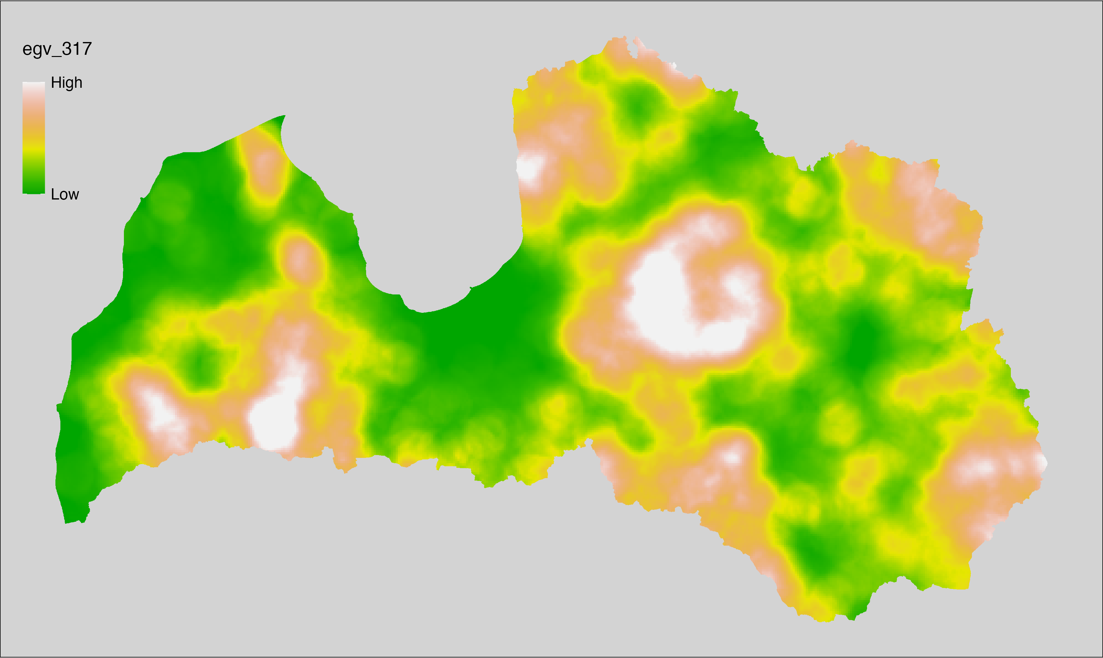
6.318 ForestsSoil_EutrophicOrganic_cell
filename: ForestsSoil_EutrophicOrganic_cell.tif
layername: egv_318
English name: Fractional cover of Eutrophic Forests on undrained Organic Soils within the analysis cell (1 ha)
Latvian name: Eitrofu mežu nesusinātās organiskajās augsnēs platības īpatsvars analīzes šūnā (1 ha)
Procedure: To prepare this EGV, forest stands with forest type equal to “15”
or “16” are selected from the State Forest Service’s State Forest
Registry and rasterised. Rasterisation is performed using
the workflow egvtools::polygon2input() with background
covering (value 0). The resulting layer
is then aggregated to EGV resolution using the workflow egvtools::input2egv(), which
calculates the arithmetic mean to determine the cover fraction. During
aggregation, inverse distance weighted (power = 2) gap filling on the output is
applied to ensure no missing values at the edges. Finally, the layer is
standardised by subtracting the arithmetic mean and dividing by the root mean squared
error.
Code
# libs ----
if(!require(egvtools)) {remotes::install_github("aavotins/egvtools"); require(egvtools)}
if(!require(terra)) {install.packages("terra"); require(terra)}
if(!require(sf)) {install.packages("sf"); require(sf)}
if(!require(tidyverse)) {install.packages("tidyverse"); require(tidyverse)}
if(!require(sfarrow)) {install.packages("sfarrow"); require(sfarrow)}
if(!require(readxl)) {install.packages("readxl"); require(readxl)}
if(!require(raster)) {install.packages("raster"); require(raster)}
if(!require(fasterize)) {install.packages("fasterize"); require(fasterize)}
# templates ----
template100=rast("./Templates/TemplateRasters/LV100m_10km.tif")
template10=rast("./Templates/TemplateRasters/LV10m_10km.tif")
rastrs10=raster(template10)
nulls10=rast("./Templates/TemplateRasters/nulls_LV10m_10km.tif")
nulls100=rast("./Templates/TemplateRasters/nulls_LV100m_10km.tif")
# simple landscape ----
simple_landscape=rast("RasterGrids_10m/2024/Ainava_vienk_mask.tif")
# mvr ----
mvr=st_read_parquet("./Geodata/2024/MVR/nogabali_2024janv.parquet")
mvr$yes=1
# ForestsSoil_EutrophicOrganic_cell.tif egv_318 ----
EutrophicOrganic=mvr %>%
filter(mt %in% c("15","16"))
p2i_rez=egvtools::polygon2input(vector_data = EutrophicOrganic,
template_path = "./Templates/TemplateRasters/LV10m_10km.tif",
out_path = "./RasterGrids_10m/2024/",
file_name = "ForestsSoil_EutrophicOrganic_input.tif",
value_field = "yes",
prepare=FALSE,
background_raster = "./Templates/TemplateRasters/nulls_LV10m_10km.tif",
plot_result = TRUE)
p2i_rez
i2e_rez=egvtools::input2egv(input=paste0("./RasterGrids_10m/2024/",
"ForestsSoil_EutrophicOrganic_input.tif"),
egv_template= "./Templates/TemplateRasters/LV100m_10km.tif",
summary_function = "average",
missing_job = "FillOutput",
outlocation = "./RasterGrids_100m/2024/RAW/",
outfilename = "ForestsSoil_EutrophicOrganic_cell.tif",
layername = "egv_318",
idw_weight = 2,
plot_gaps = FALSE,plot_final = TRUE)
i2e_rez
rm(EutrophicOrganic)
rm(p2i_rez)
rm(i2e_rez)
unlink("./RasterGrids_10m/2024/ForestsSoil_EutrophicOrganic_input.tif")
# standardisation ----
if(!require(terra)) {install.packages("terra"); require(terra)}
if(!require(tidyverse)) {install.packages("tidyverse"); require(tidyverse)}
nosaukums="ForestsSoil_EutrophicOrganic_cell.tif"
ielasisanas_cels=paste0("./RasterGrids_100m/2024/RAW/",nosaukums)
saglabasanas_cels=paste0("./RasterGrids_100m/2024/Scaled/",nosaukums)
slanis=rast(ielasisanas_cels)
videjais=global(slanis,fun="mean",na.rm=TRUE)
centrets=slanis-videjais[,1]
standartnovirze=terra::global(centrets,fun="rms",na.rm=TRUE)
merogots=centrets/standartnovirze[,1]
writeRaster(merogots,
filename=saglabasanas_cels,
overwrite=TRUE)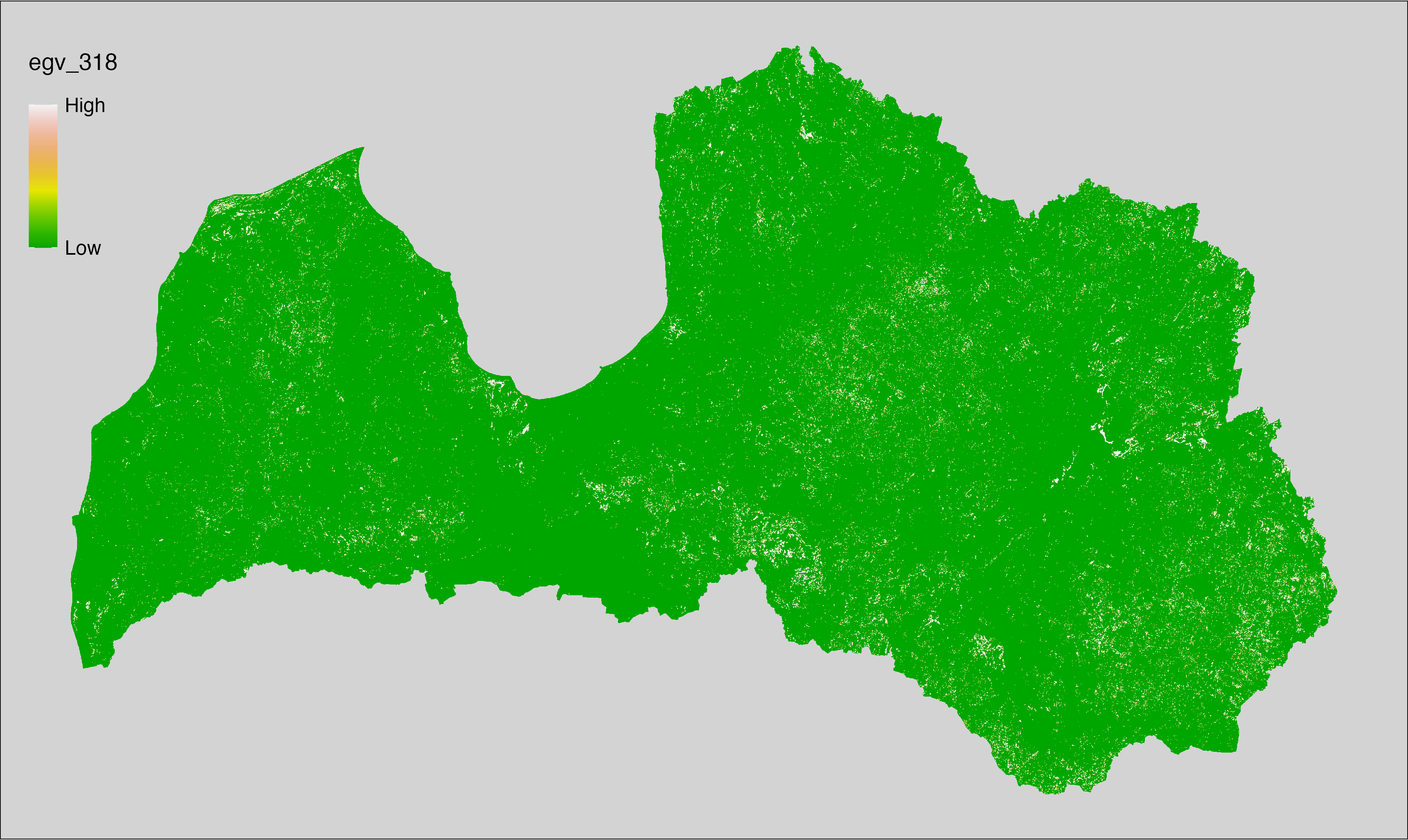
6.319 ForestsSoil_EutrophicOrganic_r500
filename: ForestsSoil_EutrophicOrganic_r500.tif
layername: egv_319
English name: Fractional cover of Eutrophic Forests on undrained Organic Soils within the 0.5 km landscape
Latvian name: Eitrofu mežu nesusinātās organiskajās augsnēs platības īpatsvars 0,5 km ainavā
Procedure: The cover fraction within a radius of 500 m around the analysis grid cell is
calculated as the area-weighted sum of the analysis cells inside the
buffer, using the workflow egvtools::radius_function(). During the calculation of the landscape metric,
inverse distance weighted (power = 2) gap filling on the output is applied
to ensure no missing values at the edges. Then the layer is rewritten to set
its name. Finally, the layer is standardised by subtracting the arithmetic
mean and dividing by the root mean squared error.
Code
# libs ----
if(!require(terra)) {install.packages("terra"); require(terra)}
if(!require(egvtools)) {remotes::install_github("aavotins/egvtools"); require(egvtools)}
# Templates -----
template100=rast("./Templates/TemplateRasters/LV100m_10km.tif")
# radii ----
radius_function(
kvadrati_path = "./Templates/TemplateGrids/tiles/",
radii_path = "./Templates/TemplateGridPoints/tiles/",
tikls100_path = "./Templates/TemplateGrids/tikls100_sauzeme.parquet",
template_path = "./Templates/TemplateRasters/LV100m_10km.tif",
input_layers = c("./RasterGrids_100m/2024/RAW/ForestsSoil_EutrophicOrganic_cell.tif"),
layer_prefixes = c("ForestsSoil_EutrophicOrganic"),
output_dir = "./RasterGrids_100m/2024/RAW/",
n_workers = 6,
radii = c("r500"),
radius_mode = "sparse",
extract_fun = "mean",
fill_missing = TRUE,
IDW_weight = 2,
future_max_size = 40 * 1024^3)
# ForestsSoil_EutrophicOrganic_r500.tif egv_319
slanis=rast("./RasterGrids_100m/2024/RAW/ForestsSoil_EutrophicOrganic_r500.tif")
names(slanis)="egv_319"
slanis2=project(slanis,template100)
writeRaster(slanis2,
"./RasterGrids_100m/2024/RAW/ForestsSoil_EutrophicOrganic_r500.tif",
overwrite=TRUE)
# standardisation ----
if(!require(terra)) {install.packages("terra"); require(terra)}
if(!require(tidyverse)) {install.packages("tidyverse"); require(tidyverse)}
nosaukums="ForestsSoil_EutrophicOrganic_r500.tif"
ielasisanas_cels=paste0("./RasterGrids_100m/2024/RAW/",nosaukums)
saglabasanas_cels=paste0("./RasterGrids_100m/2024/Scaled/",nosaukums)
slanis=rast(ielasisanas_cels)
videjais=global(slanis,fun="mean",na.rm=TRUE)
centrets=slanis-videjais[,1]
standartnovirze=terra::global(centrets,fun="rms",na.rm=TRUE)
merogots=centrets/standartnovirze[,1]
writeRaster(merogots,
filename=saglabasanas_cels,
overwrite=TRUE)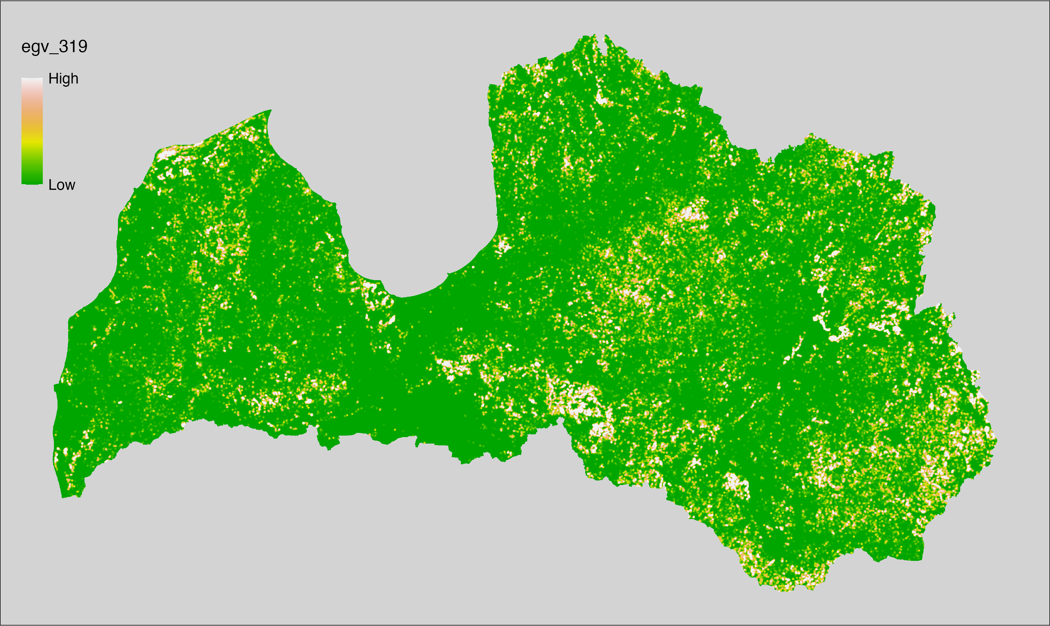
6.320 ForestsSoil_EutrophicOrganic_r1250
filename: ForestsSoil_EutrophicOrganic_r1250.tif
layername: egv_320
English name: Fractional cover of Eutrophic Forests on undrained Organic Soils within the 1.25 km landscape
Latvian name: Eitrofu mežu nesusinātās organiskajās augsnēs platības īpatsvars 1,25 km ainavā
Procedure: The cover fraction within a radius of 1250 m around the analysis grid cell
is calculated as the area-weighted sum of the analysis cells inside
the buffer, using the workflow egvtools::radius_function(). During the calculation of the landscape
metric, inverse distance weighted (power = 2) gap filling on the output is
applied to ensure no missing values at the edges. Then the layer is
rewritten to set its name. Finally, the layer is standardised by
subtracting the arithmetic mean and dividing by the root mean squared error.
Code
# libs ----
if(!require(terra)) {install.packages("terra"); require(terra)}
if(!require(egvtools)) {remotes::install_github("aavotins/egvtools"); require(egvtools)}
# Templates -----
template100=rast("./Templates/TemplateRasters/LV100m_10km.tif")
# radii ----
radius_function(
kvadrati_path = "./Templates/TemplateGrids/tiles/",
radii_path = "./Templates/TemplateGridPoints/tiles/",
tikls100_path = "./Templates/TemplateGrids/tikls100_sauzeme.parquet",
template_path = "./Templates/TemplateRasters/LV100m_10km.tif",
input_layers = c("./RasterGrids_100m/2024/RAW/ForestsSoil_EutrophicOrganic_cell.tif"),
layer_prefixes = c("ForestsSoil_EutrophicOrganic"),
output_dir = "./RasterGrids_100m/2024/RAW/",
n_workers = 6,
radii = c("r1250"),
radius_mode = "sparse",
extract_fun = "mean",
fill_missing = TRUE,
IDW_weight = 2,
future_max_size = 40 * 1024^3)
# ForestsSoil_EutrophicOrganic_r1250.tif egv_320
slanis=rast("./RasterGrids_100m/2024/RAW/ForestsSoil_EutrophicOrganic_r1250.tif")
names(slanis)="egv_320"
slanis2=project(slanis,template100)
writeRaster(slanis2,
"./RasterGrids_100m/2024/RAW/ForestsSoil_EutrophicOrganic_r1250.tif",
overwrite=TRUE)
# standardisation ----
if(!require(terra)) {install.packages("terra"); require(terra)}
if(!require(tidyverse)) {install.packages("tidyverse"); require(tidyverse)}
nosaukums="ForestsSoil_EutrophicOrganic_r1250.tif"
ielasisanas_cels=paste0("./RasterGrids_100m/2024/RAW/",nosaukums)
saglabasanas_cels=paste0("./RasterGrids_100m/2024/Scaled/",nosaukums)
slanis=rast(ielasisanas_cels)
videjais=global(slanis,fun="mean",na.rm=TRUE)
centrets=slanis-videjais[,1]
standartnovirze=terra::global(centrets,fun="rms",na.rm=TRUE)
merogots=centrets/standartnovirze[,1]
writeRaster(merogots,
filename=saglabasanas_cels,
overwrite=TRUE)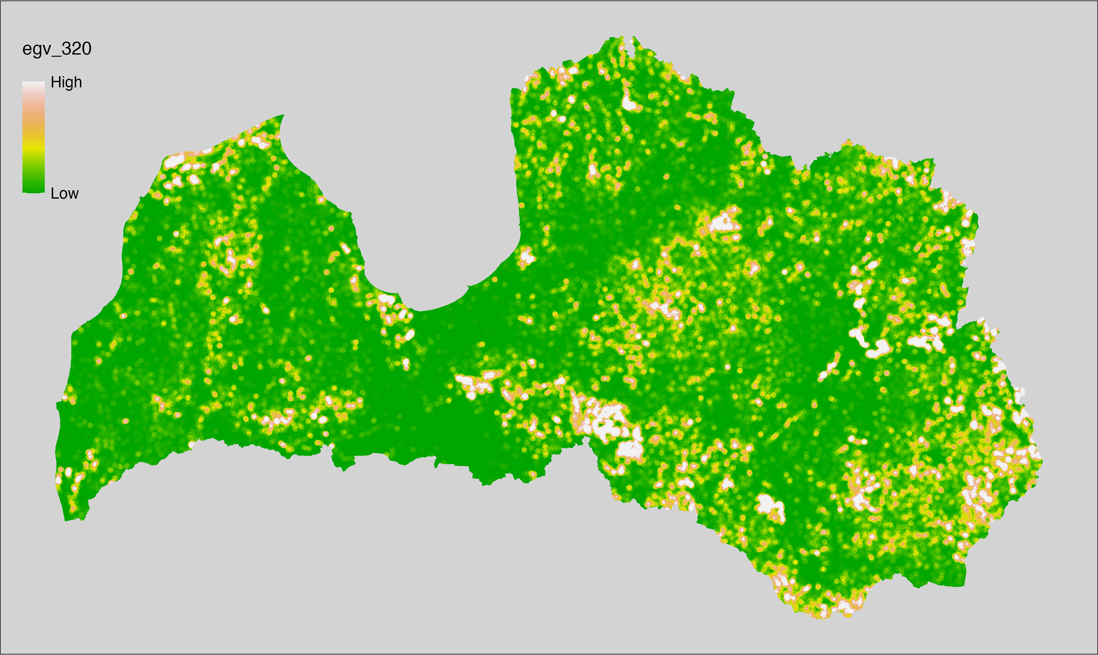
6.321 ForestsSoil_EutrophicOrganic_r3000
filename: ForestsSoil_EutrophicOrganic_r3000.tif
layername: egv_321
English name: Fractional cover of Eutrophic Forests on undrained Organic Soils within the 3 km landscape
Latvian name: Eitrofu mežu nesusinātās organiskajās augsnēs platības īpatsvars 3 km ainavā
Procedure: The cover fraction within a radius of 3000 m around the analysis grid cell
is calculated as the area-weighted sum of the analysis cells inside
the buffer, using the workflow egvtools::radius_function(). During the calculation of the landscape
metric, inverse distance weighted (power = 2) gap filling on the output is
applied to ensure no missing values at the edges. Then the layer is
rewritten to set its name. Finally, the layer is standardised by
subtracting the arithmetic mean and dividing by the root mean squared error.
Code
# libs ----
if(!require(terra)) {install.packages("terra"); require(terra)}
if(!require(egvtools)) {remotes::install_github("aavotins/egvtools"); require(egvtools)}
# Templates -----
template100=rast("./Templates/TemplateRasters/LV100m_10km.tif")
# radii ----
radius_function(
kvadrati_path = "./Templates/TemplateGrids/tiles/",
radii_path = "./Templates/TemplateGridPoints/tiles/",
tikls100_path = "./Templates/TemplateGrids/tikls100_sauzeme.parquet",
template_path = "./Templates/TemplateRasters/LV100m_10km.tif",
input_layers = c("./RasterGrids_100m/2024/RAW/ForestsSoil_EutrophicOrganic_cell.tif"),
layer_prefixes = c("ForestsSoil_EutrophicOrganic"),
output_dir = "./RasterGrids_100m/2024/RAW/",
n_workers = 6,
radii = c("r3000"),
radius_mode = "sparse",
extract_fun = "mean",
fill_missing = TRUE,
IDW_weight = 2,
future_max_size = 40 * 1024^3)
# ForestsSoil_EutrophicOrganic_r3000.tif egv_321
slanis=rast("./RasterGrids_100m/2024/RAW/ForestsSoil_EutrophicOrganic_r3000.tif")
names(slanis)="egv_321"
slanis2=project(slanis,template100)
writeRaster(slanis2,
"./RasterGrids_100m/2024/RAW/ForestsSoil_EutrophicOrganic_r3000.tif",
overwrite=TRUE)
# standardisation ----
if(!require(terra)) {install.packages("terra"); require(terra)}
if(!require(tidyverse)) {install.packages("tidyverse"); require(tidyverse)}
nosaukums="ForestsSoil_EutrophicOrganic_r3000.tif"
ielasisanas_cels=paste0("./RasterGrids_100m/2024/RAW/",nosaukums)
saglabasanas_cels=paste0("./RasterGrids_100m/2024/Scaled/",nosaukums)
slanis=rast(ielasisanas_cels)
videjais=global(slanis,fun="mean",na.rm=TRUE)
centrets=slanis-videjais[,1]
standartnovirze=terra::global(centrets,fun="rms",na.rm=TRUE)
merogots=centrets/standartnovirze[,1]
writeRaster(merogots,
filename=saglabasanas_cels,
overwrite=TRUE)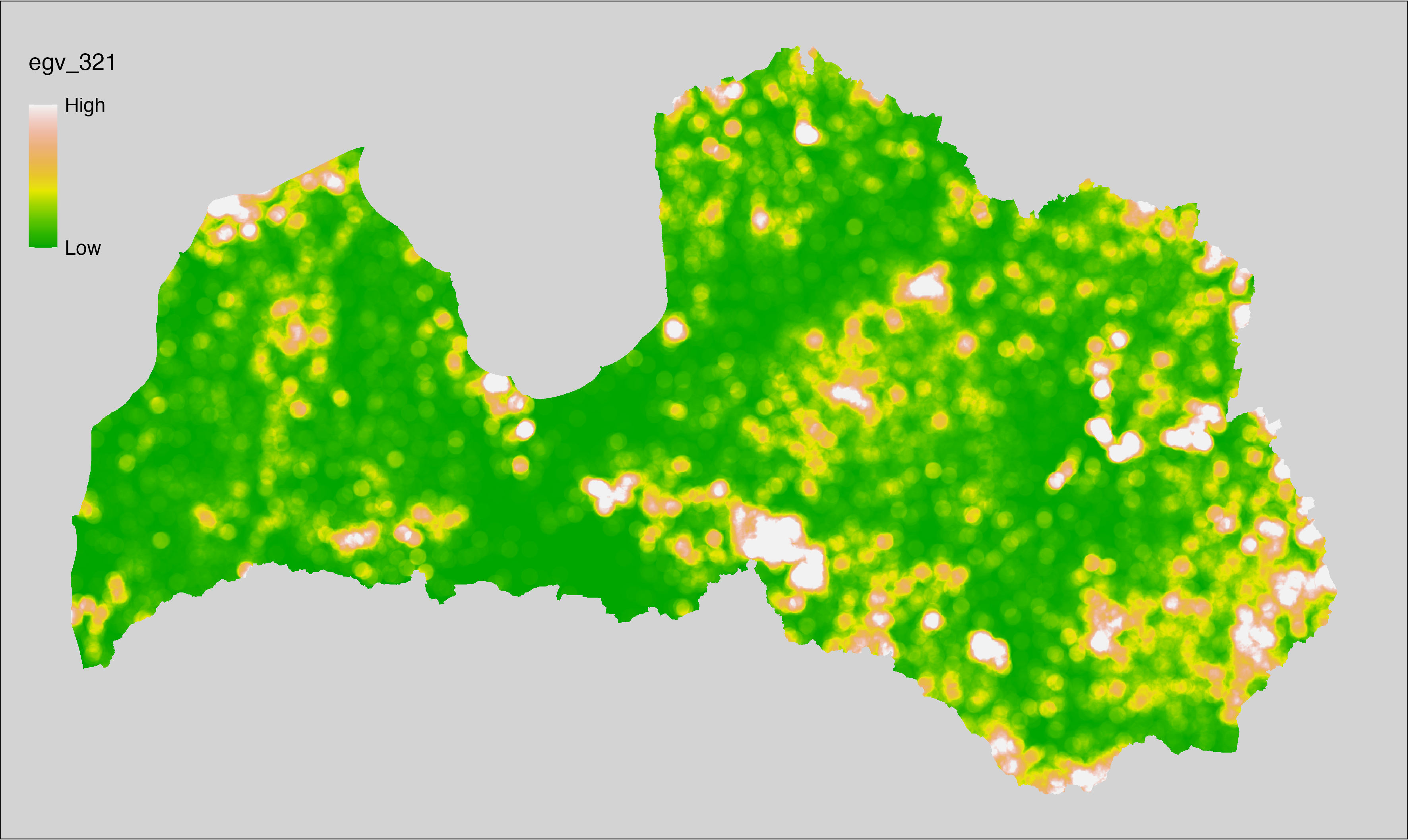
6.322 ForestsSoil_EutrophicOrganic_r10000
filename: ForestsSoil_EutrophicOrganic_r10000.tif
layername: egv_322
English name: Fractional cover of Eutrophic Forests on undrained Organic Soils within the 10 km landscape
Latvian name: Eitrofu mežu nesusinātās organiskajās augsnēs platības īpatsvars 10 km ainavā
Procedure: The cover fraction within a radius of 10000 m around the analysis grid cell
is calculated as the area-weighted sum of the analysis cells inside
the buffer, using the workflow egvtools::radius_function(). During the calculation of the landscape
metric, inverse distance weighted (power = 2) gap filling on the output is
applied to ensure no missing values at the edges. Then the layer is
rewritten to set its name. Finally, the layer is standardised by
subtracting the arithmetic mean and dividing by the root mean squared error.
Code
# libs ----
if(!require(terra)) {install.packages("terra"); require(terra)}
if(!require(egvtools)) {remotes::install_github("aavotins/egvtools"); require(egvtools)}
# Templates -----
template100=rast("./Templates/TemplateRasters/LV100m_10km.tif")
# radii ----
radius_function(
kvadrati_path = "./Templates/TemplateGrids/tiles/",
radii_path = "./Templates/TemplateGridPoints/tiles/",
tikls100_path = "./Templates/TemplateGrids/tikls100_sauzeme.parquet",
template_path = "./Templates/TemplateRasters/LV100m_10km.tif",
input_layers = c("./RasterGrids_100m/2024/RAW/ForestsSoil_EutrophicOrganic_cell.tif"),
layer_prefixes = c("ForestsSoil_EutrophicOrganic"),
output_dir = "./RasterGrids_100m/2024/RAW/",
n_workers = 6,
radii = c("r10000"),
radius_mode = "sparse",
extract_fun = "mean",
fill_missing = TRUE,
IDW_weight = 2,
future_max_size = 40 * 1024^3)
# ForestsSoil_EutrophicOrganic_r10000.tif egv_322
slanis=rast("./RasterGrids_100m/2024/RAW/ForestsSoil_EutrophicOrganic_r10000.tif")
names(slanis)="egv_322"
slanis2=project(slanis,template100)
writeRaster(slanis2,
"./RasterGrids_100m/2024/RAW/ForestsSoil_EutrophicOrganic_r10000.tif",
overwrite=TRUE)
# standardisation ----
if(!require(terra)) {install.packages("terra"); require(terra)}
if(!require(tidyverse)) {install.packages("tidyverse"); require(tidyverse)}
nosaukums="ForestsSoil_EutrophicOrganic_r10000.tif"
ielasisanas_cels=paste0("./RasterGrids_100m/2024/RAW/",nosaukums)
saglabasanas_cels=paste0("./RasterGrids_100m/2024/Scaled/",nosaukums)
slanis=rast(ielasisanas_cels)
videjais=global(slanis,fun="mean",na.rm=TRUE)
centrets=slanis-videjais[,1]
standartnovirze=terra::global(centrets,fun="rms",na.rm=TRUE)
merogots=centrets/standartnovirze[,1]
writeRaster(merogots,
filename=saglabasanas_cels,
overwrite=TRUE)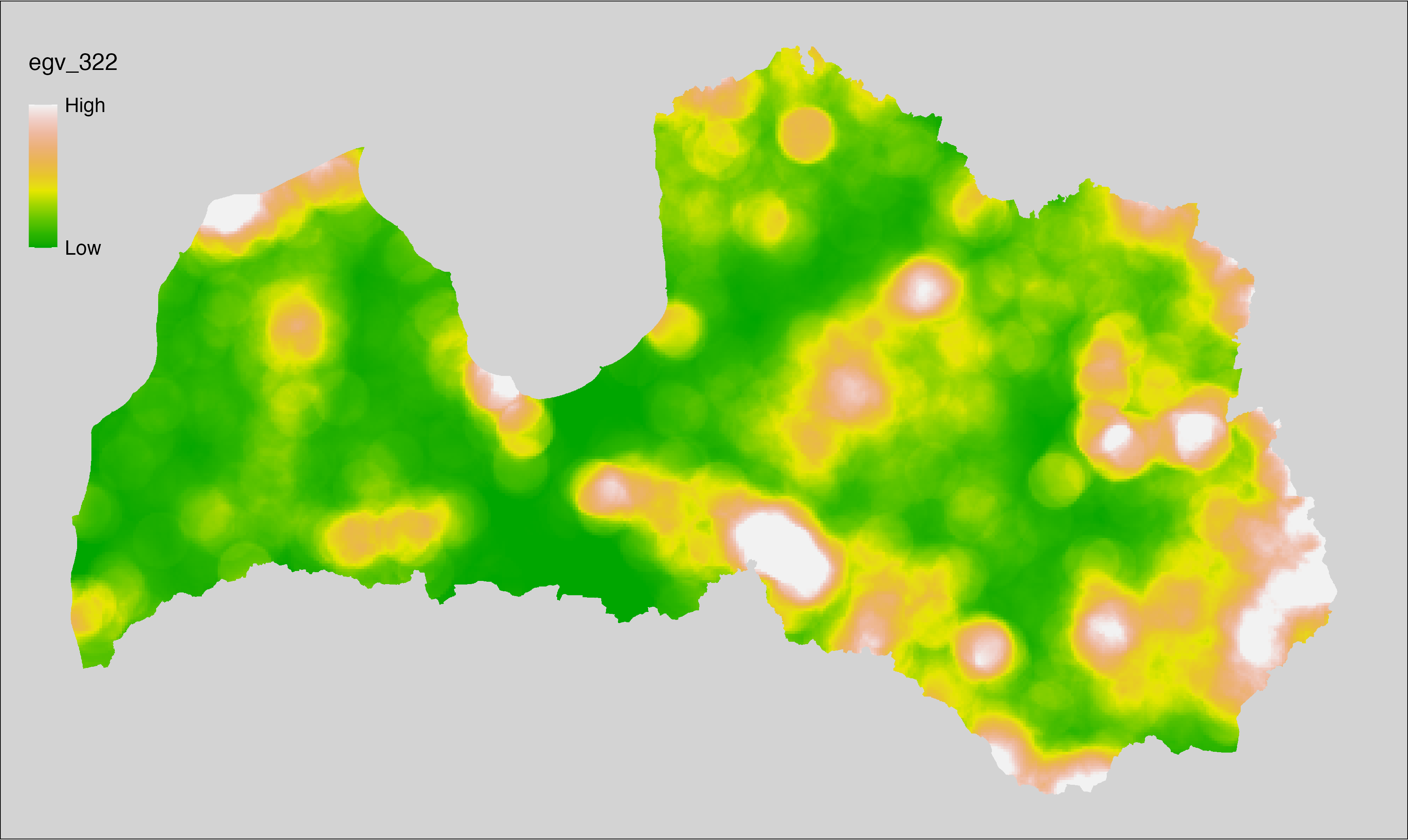
6.323 ForestsSoil_MesotrophicMineral_cell
filename: ForestsSoil_MesotrophicMineral_cell.tif
layername: egv_323
English name: Fractional cover of Mesotrophic Forests on undrained Mineral Soils within the analysis cell (1 ha)
Latvian name: Mezotrofu mežu nesusinātās minerālaugsnēs platības īpatsvars analīzes šūnā (1 ha)
Procedure: To prepare this EGV, forest stands with forest type equal to “4”
or “9” are selected from the State Forest Service’s State Forest
Registry and rasterised. Rasterisation is performed using the
workflow egvtools::polygon2input() with background
covering (value 0). The resulting layer
is then aggregated to EGV resolution using the workflow egvtools::input2egv(), which
calculates the arithmetic mean to determine the cover fraction. During
aggregation, inverse distance weighted (power = 2) gap filling on the output is
applied to ensure no missing values at the edges. Finally, the layer is
standardised by subtracting the arithmetic mean and dividing by the root mean squared
error.
Code
# libs ----
if(!require(egvtools)) {remotes::install_github("aavotins/egvtools"); require(egvtools)}
if(!require(terra)) {install.packages("terra"); require(terra)}
if(!require(sf)) {install.packages("sf"); require(sf)}
if(!require(tidyverse)) {install.packages("tidyverse"); require(tidyverse)}
if(!require(sfarrow)) {install.packages("sfarrow"); require(sfarrow)}
if(!require(readxl)) {install.packages("readxl"); require(readxl)}
if(!require(raster)) {install.packages("raster"); require(raster)}
if(!require(fasterize)) {install.packages("fasterize"); require(fasterize)}
# templates ----
template100=rast("./Templates/TemplateRasters/LV100m_10km.tif")
template10=rast("./Templates/TemplateRasters/LV10m_10km.tif")
rastrs10=raster(template10)
nulls10=rast("./Templates/TemplateRasters/nulls_LV10m_10km.tif")
nulls100=rast("./Templates/TemplateRasters/nulls_LV100m_10km.tif")
# simple landscape ----
simple_landscape=rast("RasterGrids_10m/2024/Ainava_vienk_mask.tif")
# mvr ----
mvr=st_read_parquet("./Geodata/2024/MVR/nogabali_2024janv.parquet")
mvr$yes=1
# ForestsSoil_MesotrophicMineral_cell.tif egv_323 ----
MesotrophicMineral=mvr %>%
filter(mt %in% c("4","9"))
p2i_rez=egvtools::polygon2input(vector_data = MesotrophicMineral,
template_path = "./Templates/TemplateRasters/LV10m_10km.tif",
out_path = "./RasterGrids_10m/2024/",
file_name = "ForestsSoil_MesotrophicMineral_input.tif",
value_field = "yes",
prepare=FALSE,
background_raster = "./Templates/TemplateRasters/nulls_LV10m_10km.tif",
plot_result = TRUE)
p2i_rez
i2e_rez=egvtools::input2egv(input=paste0("./RasterGrids_10m/2024/",
"ForestsSoil_MesotrophicMineral_input.tif"),
egv_template= "./Templates/TemplateRasters/LV100m_10km.tif",
summary_function = "average",
missing_job = "FillOutput",
outlocation = "./RasterGrids_100m/2024/RAW/",
outfilename = "ForestsSoil_MesotrophicMineral_cell.tif",
layername = "egv_323",
idw_weight = 2,
plot_gaps = FALSE,plot_final = TRUE)
i2e_rez
rm(MesotrophicMineral)
rm(p2i_rez)
rm(i2e_rez)
unlink("./RasterGrids_10m/2024/ForestsSoil_MesotrophicMineral_input.tif")
# standardisation ----
if(!require(terra)) {install.packages("terra"); require(terra)}
if(!require(tidyverse)) {install.packages("tidyverse"); require(tidyverse)}
nosaukums="ForestsSoil_MesotrophicMineral_cell.tif"
ielasisanas_cels=paste0("./RasterGrids_100m/2024/RAW/",nosaukums)
saglabasanas_cels=paste0("./RasterGrids_100m/2024/Scaled/",nosaukums)
slanis=rast(ielasisanas_cels)
videjais=global(slanis,fun="mean",na.rm=TRUE)
centrets=slanis-videjais[,1]
standartnovirze=terra::global(centrets,fun="rms",na.rm=TRUE)
merogots=centrets/standartnovirze[,1]
writeRaster(merogots,
filename=saglabasanas_cels,
overwrite=TRUE)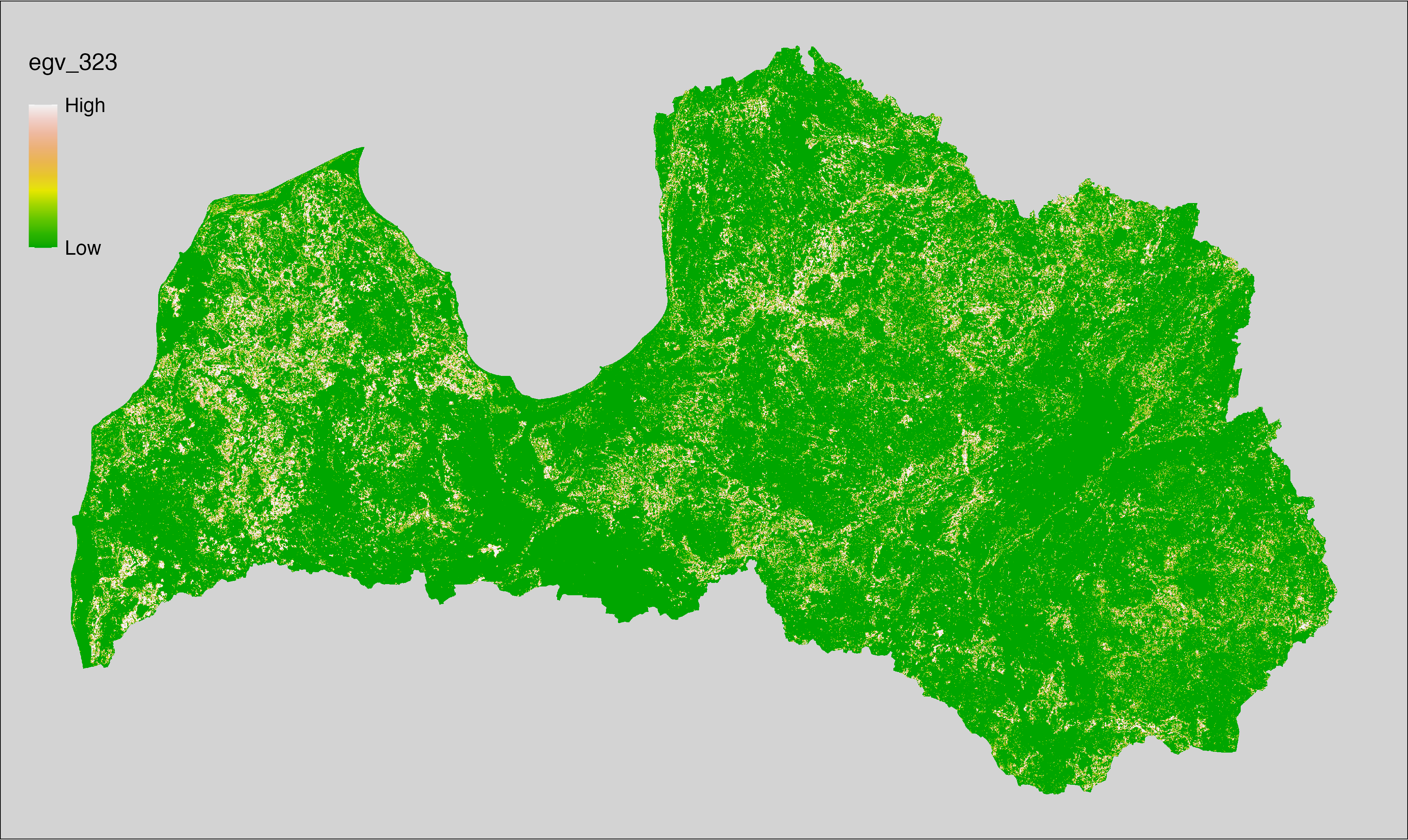
6.324 ForestsSoil_MesotrophicMineral_r500
filename: ForestsSoil_MesotrophicMineral_r500.tif
layername: egv_324
English name: Fractional cover of Mesotrophic Forests on undrained Mineral Soils within the 0.5 km landscape
Latvian name: Mezotrofu mežu nesusinātās minerālaugsnēs platības īpatsvars 0,5 km ainavā
Procedure: The cover fraction within a radius of 500 m around the analysis grid cell is
calculated as the area-weighted sum of the analysis cells inside the
buffer, using the workflow egvtools::radius_function(). During the calculation of the landscape metric,
inverse distance weighted (power = 2) gap filling on the output is applied
to ensure no missing values at the edges. Then the layer is rewritten to set
its name. Finally, the layer is standardised by subtracting the arithmetic
mean and dividing by the root mean squared error.
Code
# libs ----
if(!require(terra)) {install.packages("terra"); require(terra)}
if(!require(egvtools)) {remotes::install_github("aavotins/egvtools"); require(egvtools)}
# Templates -----
template100=rast("./Templates/TemplateRasters/LV100m_10km.tif")
# radii ----
radius_function(
kvadrati_path = "./Templates/TemplateGrids/tiles/",
radii_path = "./Templates/TemplateGridPoints/tiles/",
tikls100_path = "./Templates/TemplateGrids/tikls100_sauzeme.parquet",
template_path = "./Templates/TemplateRasters/LV100m_10km.tif",
input_layers = c("./RasterGrids_100m/2024/RAW/ForestsSoil_MesotrophicMineral_cell.tif"),
layer_prefixes = c("ForestsSoil_MesotrophicMineral"),
output_dir = "./RasterGrids_100m/2024/RAW/",
n_workers = 6,
radii = c("r500"),
radius_mode = "sparse",
extract_fun = "mean",
fill_missing = TRUE,
IDW_weight = 2,
future_max_size = 40 * 1024^3)
# ForestsSoil_MesotrophicMineral_r500.tif egv_324
slanis=rast("./RasterGrids_100m/2024/RAW/ForestsSoil_MesotrophicMineral_r500.tif")
names(slanis)="egv_324"
slanis2=project(slanis,template100)
writeRaster(slanis2,
"./RasterGrids_100m/2024/RAW/ForestsSoil_MesotrophicMineral_r500.tif",
overwrite=TRUE)
# standardisation ----
if(!require(terra)) {install.packages("terra"); require(terra)}
if(!require(tidyverse)) {install.packages("tidyverse"); require(tidyverse)}
nosaukums="ForestsSoil_MesotrophicMineral_r500.tif"
ielasisanas_cels=paste0("./RasterGrids_100m/2024/RAW/",nosaukums)
saglabasanas_cels=paste0("./RasterGrids_100m/2024/Scaled/",nosaukums)
slanis=rast(ielasisanas_cels)
videjais=global(slanis,fun="mean",na.rm=TRUE)
centrets=slanis-videjais[,1]
standartnovirze=terra::global(centrets,fun="rms",na.rm=TRUE)
merogots=centrets/standartnovirze[,1]
writeRaster(merogots,
filename=saglabasanas_cels,
overwrite=TRUE)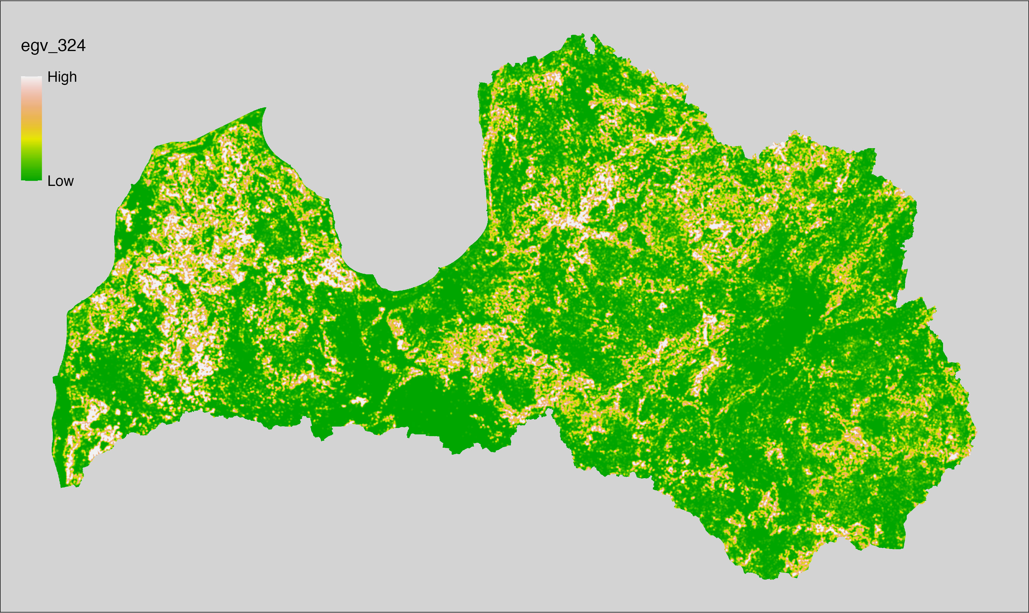
6.325 ForestsSoil_MesotrophicMineral_r1250
filename: ForestsSoil_MesotrophicMineral_r1250.tif
layername: egv_325
English name: Fractional cover of Mesotrophic Forests on undrained Mineral Soils within the 1.25 km landscape
Latvian name: Mezotrofu mežu nesusinātās minerālaugsnēs platības īpatsvars 1,25 km ainavā
Procedure: The cover fraction within a radius of 1250 m around the analysis grid cell
is calculated as the area-weighted sum of the analysis cells inside
the buffer, using the workflow egvtools::radius_function(). During the calculation of the landscape
metric, inverse distance weighted (power = 2) gap filling on the output is
applied to ensure no missing values at the edges. Then the layer is
rewritten to set its name. Finally, the layer is standardised by
subtracting the arithmetic mean and dividing by the root mean squared error.
Code
# libs ----
if(!require(terra)) {install.packages("terra"); require(terra)}
if(!require(egvtools)) {remotes::install_github("aavotins/egvtools"); require(egvtools)}
# Templates -----
template100=rast("./Templates/TemplateRasters/LV100m_10km.tif")
# radii ----
radius_function(
kvadrati_path = "./Templates/TemplateGrids/tiles/",
radii_path = "./Templates/TemplateGridPoints/tiles/",
tikls100_path = "./Templates/TemplateGrids/tikls100_sauzeme.parquet",
template_path = "./Templates/TemplateRasters/LV100m_10km.tif",
input_layers = c("./RasterGrids_100m/2024/RAW/ForestsSoil_MesotrophicMineral_cell.tif"),
layer_prefixes = c("ForestsSoil_MesotrophicMineral"),
output_dir = "./RasterGrids_100m/2024/RAW/",
n_workers = 6,
radii = c("r1250"),
radius_mode = "sparse",
extract_fun = "mean",
fill_missing = TRUE,
IDW_weight = 2,
future_max_size = 40 * 1024^3)
# ForestsSoil_MesotrophicMineral_r1250.tif egv_325
slanis=rast("./RasterGrids_100m/2024/RAW/ForestsSoil_MesotrophicMineral_r1250.tif")
names(slanis)="egv_325"
slanis2=project(slanis,template100)
writeRaster(slanis2,
"./RasterGrids_100m/2024/RAW/ForestsSoil_MesotrophicMineral_r1250.tif",
overwrite=TRUE)
# standardisation ----
if(!require(terra)) {install.packages("terra"); require(terra)}
if(!require(tidyverse)) {install.packages("tidyverse"); require(tidyverse)}
nosaukums="ForestsSoil_MesotrophicMineral_r1250.tif"
ielasisanas_cels=paste0("./RasterGrids_100m/2024/RAW/",nosaukums)
saglabasanas_cels=paste0("./RasterGrids_100m/2024/Scaled/",nosaukums)
slanis=rast(ielasisanas_cels)
videjais=global(slanis,fun="mean",na.rm=TRUE)
centrets=slanis-videjais[,1]
standartnovirze=terra::global(centrets,fun="rms",na.rm=TRUE)
merogots=centrets/standartnovirze[,1]
writeRaster(merogots,
filename=saglabasanas_cels,
overwrite=TRUE)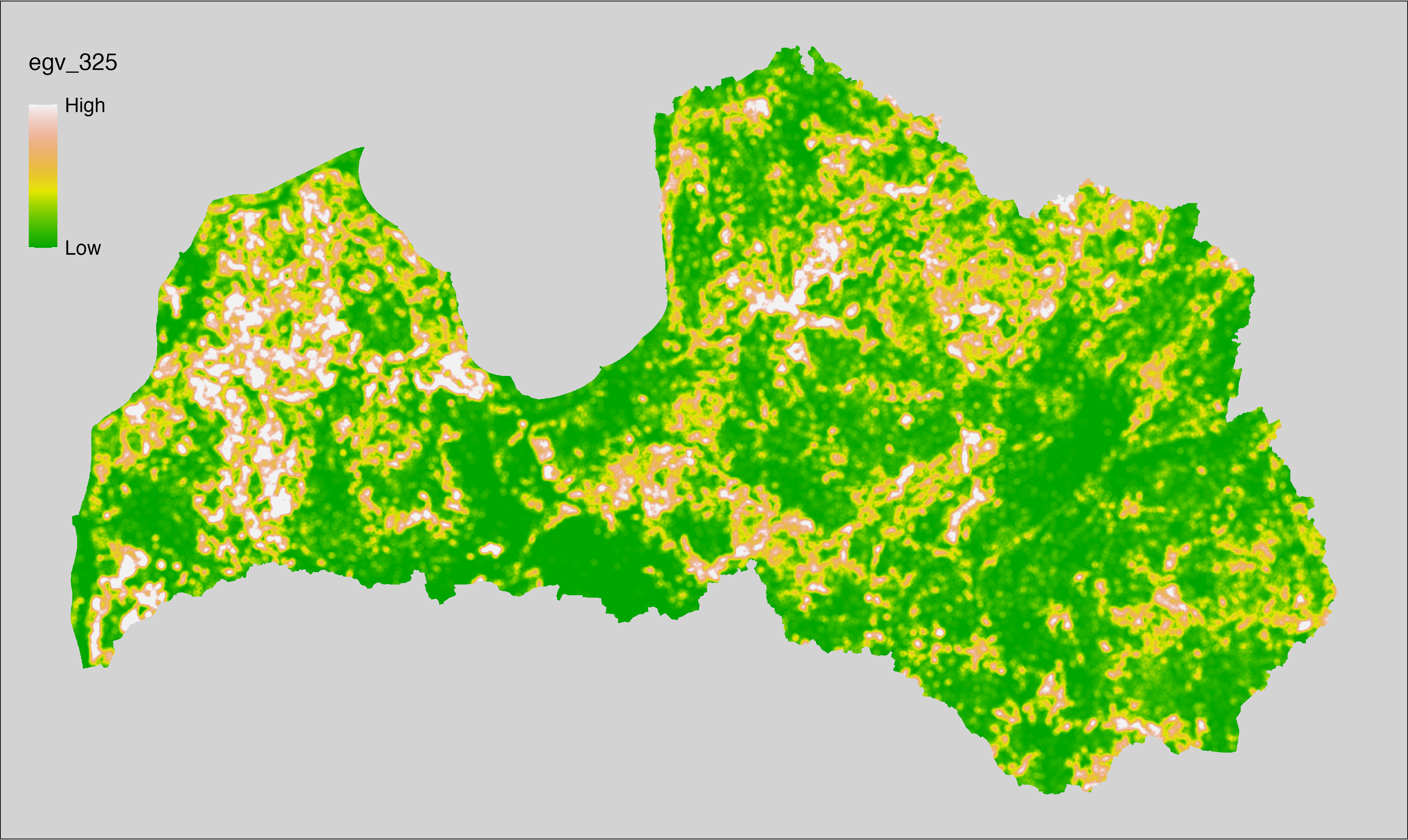
6.326 ForestsSoil_MesotrophicMineral_r3000
filename: ForestsSoil_MesotrophicMineral_r3000.tif
layername: egv_326
English name: Fractional cover of Mesotrophic Forests on undrained Mineral Soils within the 3 km landscape
Latvian name: Mezotrofu mežu nesusinātās minerālaugsnēs platības īpatsvars 3 km ainavā
Procedure: The cover fraction within a radius of 3000 m around the analysis grid cell
is calculated as the area-weighted sum of the analysis cells inside
the buffer, using the workflow egvtools::radius_function(). During the calculation of the landscape
metric, inverse distance weighted (power = 2) gap filling on the output is
applied to ensure no missing values at the edges. Then the layer is
rewritten to set its name. Finally, the layer is standardised by
subtracting the arithmetic mean and dividing by the root mean squared error.
Code
# libs ----
if(!require(terra)) {install.packages("terra"); require(terra)}
if(!require(egvtools)) {remotes::install_github("aavotins/egvtools"); require(egvtools)}
# Templates -----
template100=rast("./Templates/TemplateRasters/LV100m_10km.tif")
# radii ----
radius_function(
kvadrati_path = "./Templates/TemplateGrids/tiles/",
radii_path = "./Templates/TemplateGridPoints/tiles/",
tikls100_path = "./Templates/TemplateGrids/tikls100_sauzeme.parquet",
template_path = "./Templates/TemplateRasters/LV100m_10km.tif",
input_layers = c("./RasterGrids_100m/2024/RAW/ForestsSoil_MesotrophicMineral_cell.tif"),
layer_prefixes = c("ForestsSoil_MesotrophicMineral"),
output_dir = "./RasterGrids_100m/2024/RAW/",
n_workers = 6,
radii = c("r3000"),
radius_mode = "sparse",
extract_fun = "mean",
fill_missing = TRUE,
IDW_weight = 2,
future_max_size = 40 * 1024^3)
# ForestsSoil_MesotrophicMineral_r3000.tif egv_326
slanis=rast("./RasterGrids_100m/2024/RAW/ForestsSoil_MesotrophicMineral_r3000.tif")
names(slanis)="egv_326"
slanis2=project(slanis,template100)
writeRaster(slanis2,
"./RasterGrids_100m/2024/RAW/ForestsSoil_MesotrophicMineral_r3000.tif",
overwrite=TRUE)
# standardisation ----
if(!require(terra)) {install.packages("terra"); require(terra)}
if(!require(tidyverse)) {install.packages("tidyverse"); require(tidyverse)}
nosaukums="ForestsSoil_MesotrophicMineral_r3000.tif"
ielasisanas_cels=paste0("./RasterGrids_100m/2024/RAW/",nosaukums)
saglabasanas_cels=paste0("./RasterGrids_100m/2024/Scaled/",nosaukums)
slanis=rast(ielasisanas_cels)
videjais=global(slanis,fun="mean",na.rm=TRUE)
centrets=slanis-videjais[,1]
standartnovirze=terra::global(centrets,fun="rms",na.rm=TRUE)
merogots=centrets/standartnovirze[,1]
writeRaster(merogots,
filename=saglabasanas_cels,
overwrite=TRUE)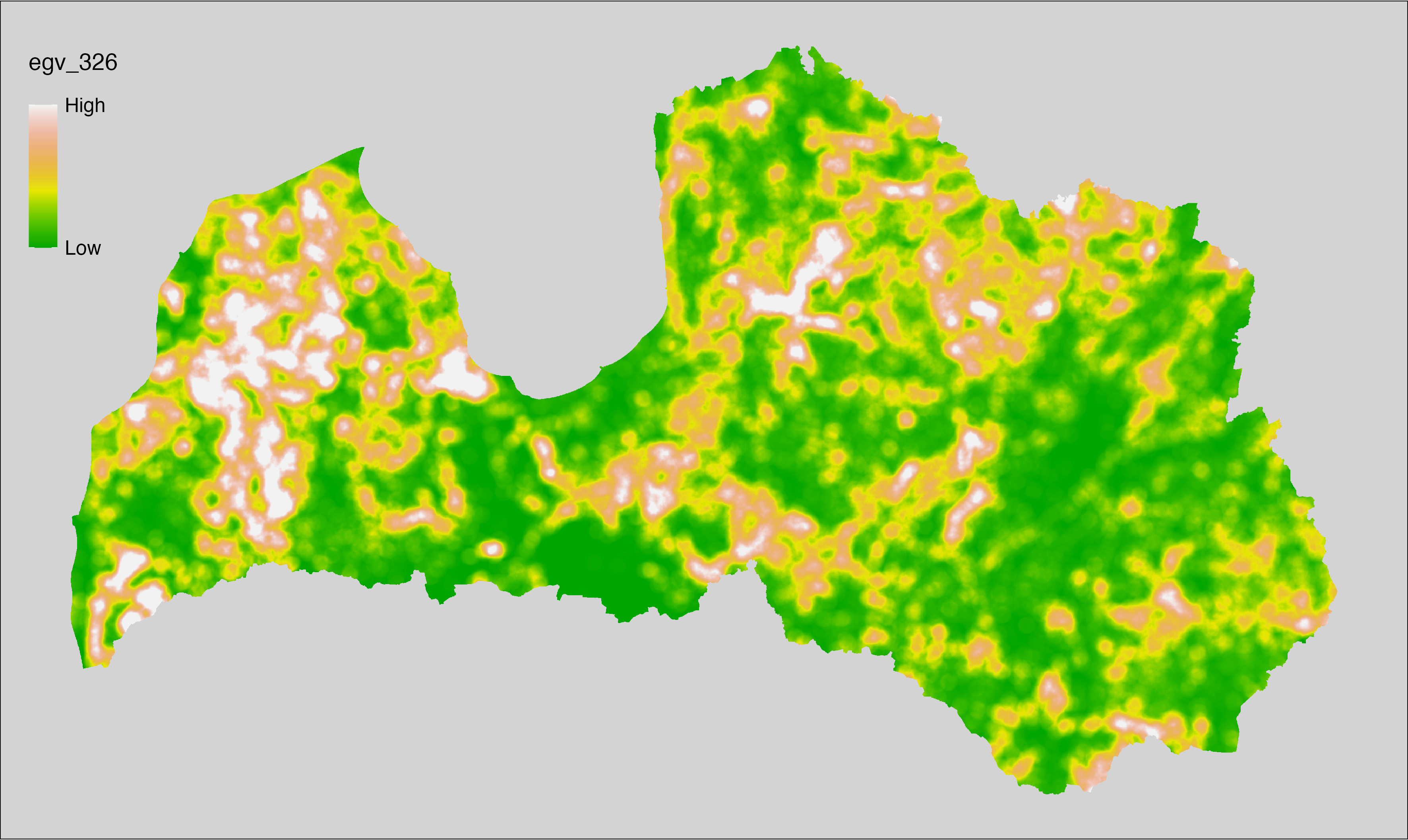
6.327 ForestsSoil_MesotrophicMineral_r10000
filename: ForestsSoil_MesotrophicMineral_r10000.tif
layername: egv_327
English name: Fractional cover of Mesotrophic Forests on undrained Mineral Soils within the 10 km landscape
Latvian name: Mezotrofu mežu nesusinātās minerālaugsnēs platības īpatsvars 10 km ainavā
Procedure: The cover fraction within a radius of 10000 m around the analysis grid cell
is calculated as the area-weighted sum of the analysis cells inside
the buffer, using the workflow egvtools::radius_function(). During the calculation of the landscape
metric, inverse distance weighted (power = 2) gap filling on the output is
applied to ensure no missing values at the edges. Then the layer is
rewritten to set its name. Finally, the layer is standardised by
subtracting the arithmetic mean and dividing by the root mean squared error.
Code
# libs ----
if(!require(terra)) {install.packages("terra"); require(terra)}
if(!require(egvtools)) {remotes::install_github("aavotins/egvtools"); require(egvtools)}
# Templates -----
template100=rast("./Templates/TemplateRasters/LV100m_10km.tif")
# radii ----
radius_function(
kvadrati_path = "./Templates/TemplateGrids/tiles/",
radii_path = "./Templates/TemplateGridPoints/tiles/",
tikls100_path = "./Templates/TemplateGrids/tikls100_sauzeme.parquet",
template_path = "./Templates/TemplateRasters/LV100m_10km.tif",
input_layers = c("./RasterGrids_100m/2024/RAW/ForestsSoil_MesotrophicMineral_cell.tif"),
layer_prefixes = c("ForestsSoil_MesotrophicMineral"),
output_dir = "./RasterGrids_100m/2024/RAW/",
n_workers = 6,
radii = c("r10000"),
radius_mode = "sparse",
extract_fun = "mean",
fill_missing = TRUE,
IDW_weight = 2,
future_max_size = 40 * 1024^3)
# ForestsSoil_MesotrophicMineral_r10000.tif egv_327
slanis=rast("./RasterGrids_100m/2024/RAW/ForestsSoil_MesotrophicMineral_r10000.tif")
names(slanis)="egv_327"
slanis2=project(slanis,template100)
writeRaster(slanis2,
"./RasterGrids_100m/2024/RAW/ForestsSoil_MesotrophicMineral_r10000.tif",
overwrite=TRUE)
# standardisation ----
if(!require(terra)) {install.packages("terra"); require(terra)}
if(!require(tidyverse)) {install.packages("tidyverse"); require(tidyverse)}
nosaukums="ForestsSoil_MesotrophicMineral_r10000.tif"
ielasisanas_cels=paste0("./RasterGrids_100m/2024/RAW/",nosaukums)
saglabasanas_cels=paste0("./RasterGrids_100m/2024/Scaled/",nosaukums)
slanis=rast(ielasisanas_cels)
videjais=global(slanis,fun="mean",na.rm=TRUE)
centrets=slanis-videjais[,1]
standartnovirze=terra::global(centrets,fun="rms",na.rm=TRUE)
merogots=centrets/standartnovirze[,1]
writeRaster(merogots,
filename=saglabasanas_cels,
overwrite=TRUE)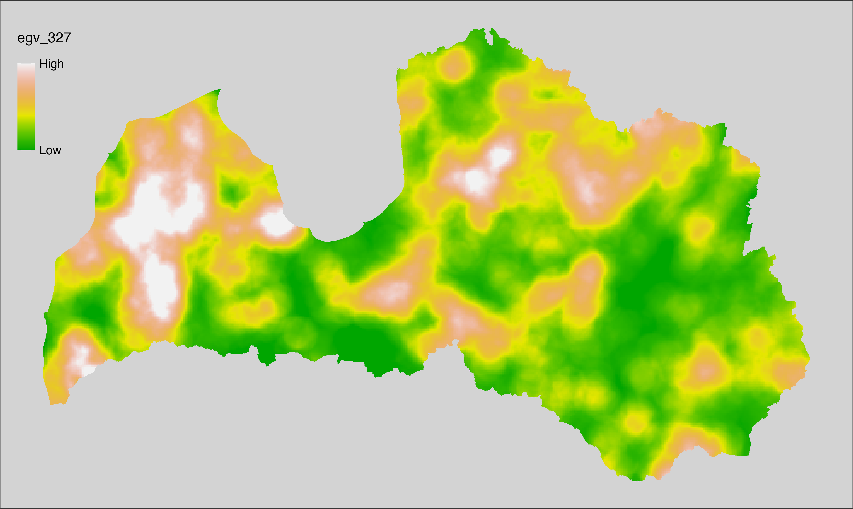
6.328 ForestsSoil_OligotrophicDrained_cell
filename: ForestsSoil_OligotrophicDrained_cell.tif
layername: egv_328
English name: Fractional cover of Drained Oligotrophic Forests within the analysis cell (1 ha)
Latvian name: Susinātu oligotrofu mežu platības īpatsvars analīzes šūnā (1 ha)
Procedure: To prepare this EGV, forest stands with forest type equal to
“17”, “18”, “22” or “23” are selected from the State Forest Service’s State Forest
Registry and rasterised. Rasterisation is performed using
the workflow egvtools::polygon2input() with background
covering (value 0). The resulting layer
is then aggregated to EGV resolution using the workflow egvtools::input2egv(), which
calculates the arithmetic mean to determine the cover fraction. During
aggregation, inverse distance weighted (power = 2) gap filling on the output is
applied to ensure no missing values at the edges. Finally, the layer is
standardised by subtracting the arithmetic mean and dividing by the root mean squared
error.
Code
# libs ----
if(!require(egvtools)) {remotes::install_github("aavotins/egvtools"); require(egvtools)}
if(!require(terra)) {install.packages("terra"); require(terra)}
if(!require(sf)) {install.packages("sf"); require(sf)}
if(!require(tidyverse)) {install.packages("tidyverse"); require(tidyverse)}
if(!require(sfarrow)) {install.packages("sfarrow"); require(sfarrow)}
if(!require(readxl)) {install.packages("readxl"); require(readxl)}
if(!require(raster)) {install.packages("raster"); require(raster)}
if(!require(fasterize)) {install.packages("fasterize"); require(fasterize)}
# templates ----
template100=rast("./Templates/TemplateRasters/LV100m_10km.tif")
template10=rast("./Templates/TemplateRasters/LV10m_10km.tif")
rastrs10=raster(template10)
nulls10=rast("./Templates/TemplateRasters/nulls_LV10m_10km.tif")
nulls100=rast("./Templates/TemplateRasters/nulls_LV100m_10km.tif")
# simple landscape ----
simple_landscape=rast("RasterGrids_10m/2024/Ainava_vienk_mask.tif")
# mvr ----
mvr=st_read_parquet("./Geodata/2024/MVR/nogabali_2024janv.parquet")
mvr$yes=1
# ForestsSoil_OligotrophicDrained_cell.tif egv_328 ----
OligotrophicDrained=mvr %>%
filter(mt %in% c("17","18","22","23"))
p2i_rez=egvtools::polygon2input(vector_data = OligotrophicDrained,
template_path = "./Templates/TemplateRasters/LV10m_10km.tif",
out_path = "./RasterGrids_10m/2024/",
file_name = "ForestsSoil_OligotrophicDrained_input.tif",
value_field = "yes",
prepare=FALSE,
background_raster = "./Templates/TemplateRasters/nulls_LV10m_10km.tif",
plot_result = TRUE)
p2i_rez
i2e_rez=egvtools::input2egv(input=paste0("./RasterGrids_10m/2024/",
"ForestsSoil_OligotrophicDrained_input.tif"),
egv_template= "./Templates/TemplateRasters/LV100m_10km.tif",
summary_function = "average",
missing_job = "FillOutput",
outlocation = "./RasterGrids_100m/2024/RAW/",
outfilename = "ForestsSoil_OligotrophicDrained_cell.tif",
layername = "egv_328",
idw_weight = 2,
plot_gaps = FALSE,plot_final = TRUE)
i2e_rez
rm(OligotrophicDrained)
rm(p2i_rez)
rm(i2e_rez)
unlink("./RasterGrids_10m/2024/ForestsSoil_OligotrophicDrained_input.tif")
# standardisation ----
if(!require(terra)) {install.packages("terra"); require(terra)}
if(!require(tidyverse)) {install.packages("tidyverse"); require(tidyverse)}
nosaukums="ForestsSoil_OligotrophicDrained_cell.tif"
ielasisanas_cels=paste0("./RasterGrids_100m/2024/RAW/",nosaukums)
saglabasanas_cels=paste0("./RasterGrids_100m/2024/Scaled/",nosaukums)
slanis=rast(ielasisanas_cels)
videjais=global(slanis,fun="mean",na.rm=TRUE)
centrets=slanis-videjais[,1]
standartnovirze=terra::global(centrets,fun="rms",na.rm=TRUE)
merogots=centrets/standartnovirze[,1]
writeRaster(merogots,
filename=saglabasanas_cels,
overwrite=TRUE)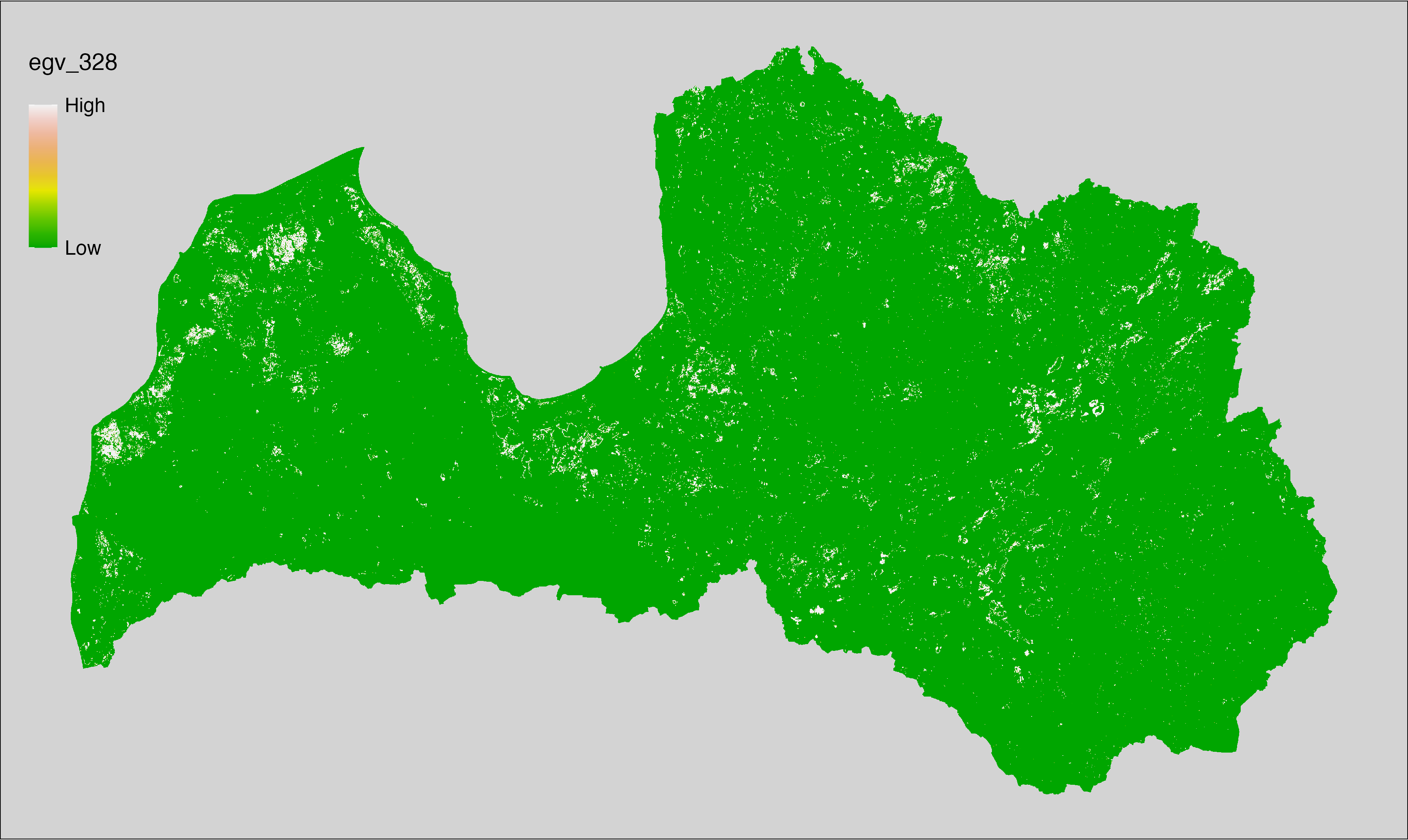
6.329 ForestsSoil_OligotrophicDrained_r500
filename: ForestsSoil_OligotrophicDrained_r500.tif
layername: egv_329
English name: Fractional cover of Drained Oligotrophic Forests within the 0.5 km landscape
Latvian name: Susinātu oligotrofu mežu platības īpatsvars 0,5 km ainavā
Procedure: The cover fraction within a radius of 500 m around the analysis grid cell is
calculated as the area-weighted sum of the analysis cells inside the
buffer, using the workflow egvtools::radius_function(). During the calculation of the landscape metric,
inverse distance weighted (power = 2) gap filling on the output is applied
to ensure no missing values at the edges. Then the layer is rewritten to set
its name. Finally, the layer is standardised by subtracting the arithmetic
mean and dividing by the root mean squared error.
Code
# libs ----
if(!require(terra)) {install.packages("terra"); require(terra)}
if(!require(egvtools)) {remotes::install_github("aavotins/egvtools"); require(egvtools)}
# Templates -----
template100=rast("./Templates/TemplateRasters/LV100m_10km.tif")
# radii ----
radius_function(
kvadrati_path = "./Templates/TemplateGrids/tiles/",
radii_path = "./Templates/TemplateGridPoints/tiles/",
tikls100_path = "./Templates/TemplateGrids/tikls100_sauzeme.parquet",
template_path = "./Templates/TemplateRasters/LV100m_10km.tif",
input_layers = c("./RasterGrids_100m/2024/RAW/ForestsSoil_OligotrophicDrained_cell.tif"),
layer_prefixes = c("ForestsSoil_OligotrophicDrained"),
output_dir = "./RasterGrids_100m/2024/RAW/",
n_workers = 6,
radii = c("r500"),
radius_mode = "sparse",
extract_fun = "mean",
fill_missing = TRUE,
IDW_weight = 2,
future_max_size = 40 * 1024^3)
# ForestsSoil_OligotrophicDrained_r500.tif egv_329
slanis=rast("./RasterGrids_100m/2024/RAW/ForestsSoil_OligotrophicDrained_r500.tif")
names(slanis)="egv_329"
slanis2=project(slanis,template100)
writeRaster(slanis2,
"./RasterGrids_100m/2024/RAW/ForestsSoil_OligotrophicDrained_r500.tif",
overwrite=TRUE)
# standardisation ----
if(!require(terra)) {install.packages("terra"); require(terra)}
if(!require(tidyverse)) {install.packages("tidyverse"); require(tidyverse)}
nosaukums="ForestsSoil_OligotrophicDrained_r500.tif"
ielasisanas_cels=paste0("./RasterGrids_100m/2024/RAW/",nosaukums)
saglabasanas_cels=paste0("./RasterGrids_100m/2024/Scaled/",nosaukums)
slanis=rast(ielasisanas_cels)
videjais=global(slanis,fun="mean",na.rm=TRUE)
centrets=slanis-videjais[,1]
standartnovirze=terra::global(centrets,fun="rms",na.rm=TRUE)
merogots=centrets/standartnovirze[,1]
writeRaster(merogots,
filename=saglabasanas_cels,
overwrite=TRUE)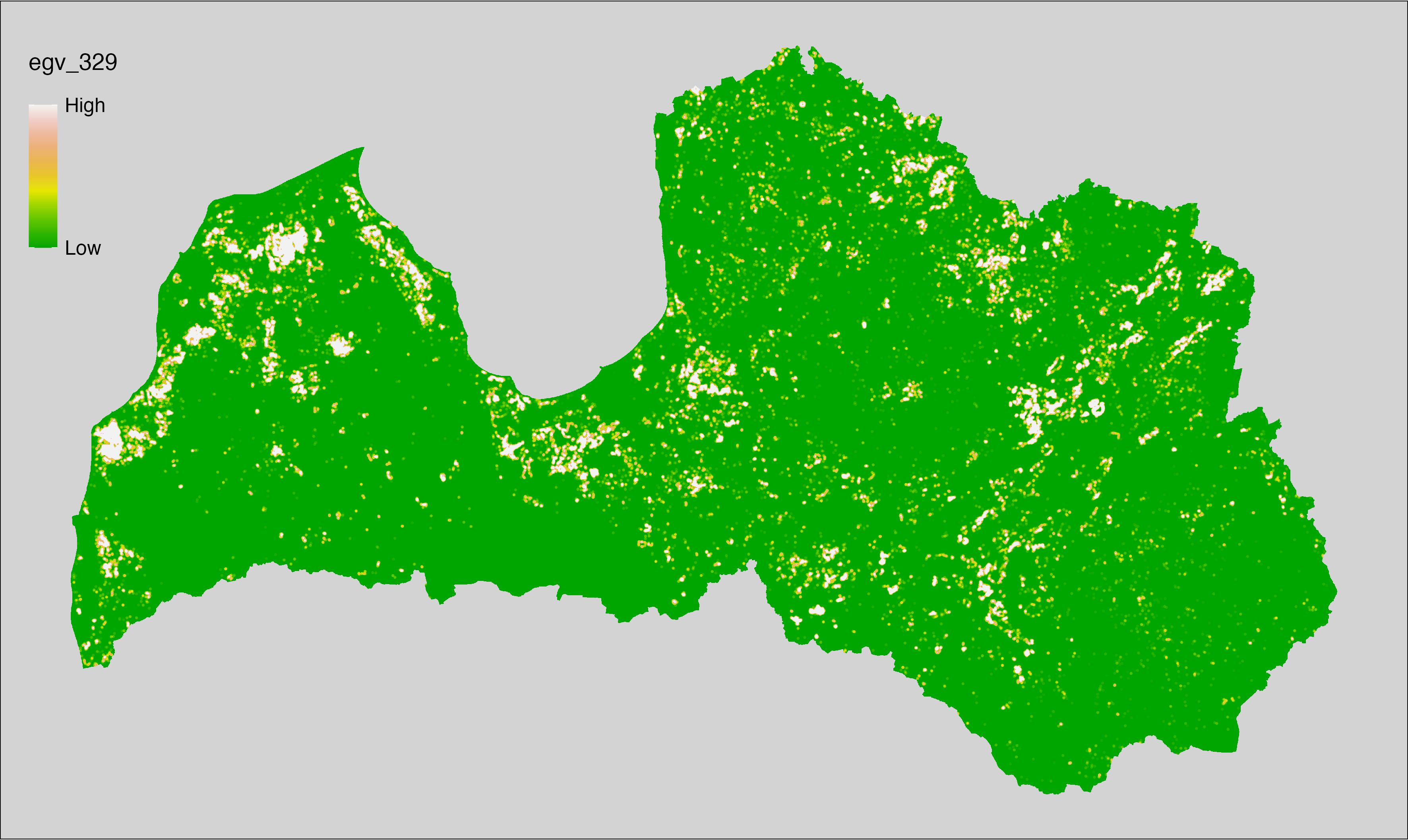
6.330 ForestsSoil_OligotrophicDrained_r1250
filename: ForestsSoil_OligotrophicDrained_r1250.tif
layername: egv_330
English name: Fractional cover of Drained Oligotrophic Forests within the 1.25 km landscape
Latvian name: Susinātu oligotrofu mežu platības īpatsvars 1,25 km ainavā
Procedure: The cover fraction within a radius of 1250 m around the analysis grid cell
is calculated as the area-weighted sum of the analysis cells inside
the buffer, using the workflow egvtools::radius_function(). During the calculation of the landscape
metric, inverse distance weighted (power = 2) gap filling on the output is
applied to ensure no missing values at the edges. Then the layer is
rewritten to set its name. Finally, the layer is standardised by
subtracting the arithmetic mean and dividing by the root mean squared error.
Code
# libs ----
if(!require(terra)) {install.packages("terra"); require(terra)}
if(!require(egvtools)) {remotes::install_github("aavotins/egvtools"); require(egvtools)}
# Templates -----
template100=rast("./Templates/TemplateRasters/LV100m_10km.tif")
# radii ----
radius_function(
kvadrati_path = "./Templates/TemplateGrids/tiles/",
radii_path = "./Templates/TemplateGridPoints/tiles/",
tikls100_path = "./Templates/TemplateGrids/tikls100_sauzeme.parquet",
template_path = "./Templates/TemplateRasters/LV100m_10km.tif",
input_layers = c("./RasterGrids_100m/2024/RAW/ForestsSoil_OligotrophicDrained_cell.tif"),
layer_prefixes = c("ForestsSoil_OligotrophicDrained"),
output_dir = "./RasterGrids_100m/2024/RAW/",
n_workers = 6,
radii = c("r1250"),
radius_mode = "sparse",
extract_fun = "mean",
fill_missing = TRUE,
IDW_weight = 2,
future_max_size = 40 * 1024^3)
# ForestsSoil_OligotrophicDrained_r1250.tif egv_330
slanis=rast("./RasterGrids_100m/2024/RAW/ForestsSoil_OligotrophicDrained_r1250.tif")
names(slanis)="egv_330"
slanis2=project(slanis,template100)
writeRaster(slanis2,
"./RasterGrids_100m/2024/RAW/ForestsSoil_OligotrophicDrained_r1250.tif",
overwrite=TRUE)
# standardisation ----
if(!require(terra)) {install.packages("terra"); require(terra)}
if(!require(tidyverse)) {install.packages("tidyverse"); require(tidyverse)}
nosaukums="ForestsSoil_OligotrophicDrained_r1250.tif"
ielasisanas_cels=paste0("./RasterGrids_100m/2024/RAW/",nosaukums)
saglabasanas_cels=paste0("./RasterGrids_100m/2024/Scaled/",nosaukums)
slanis=rast(ielasisanas_cels)
videjais=global(slanis,fun="mean",na.rm=TRUE)
centrets=slanis-videjais[,1]
standartnovirze=terra::global(centrets,fun="rms",na.rm=TRUE)
merogots=centrets/standartnovirze[,1]
writeRaster(merogots,
filename=saglabasanas_cels,
overwrite=TRUE)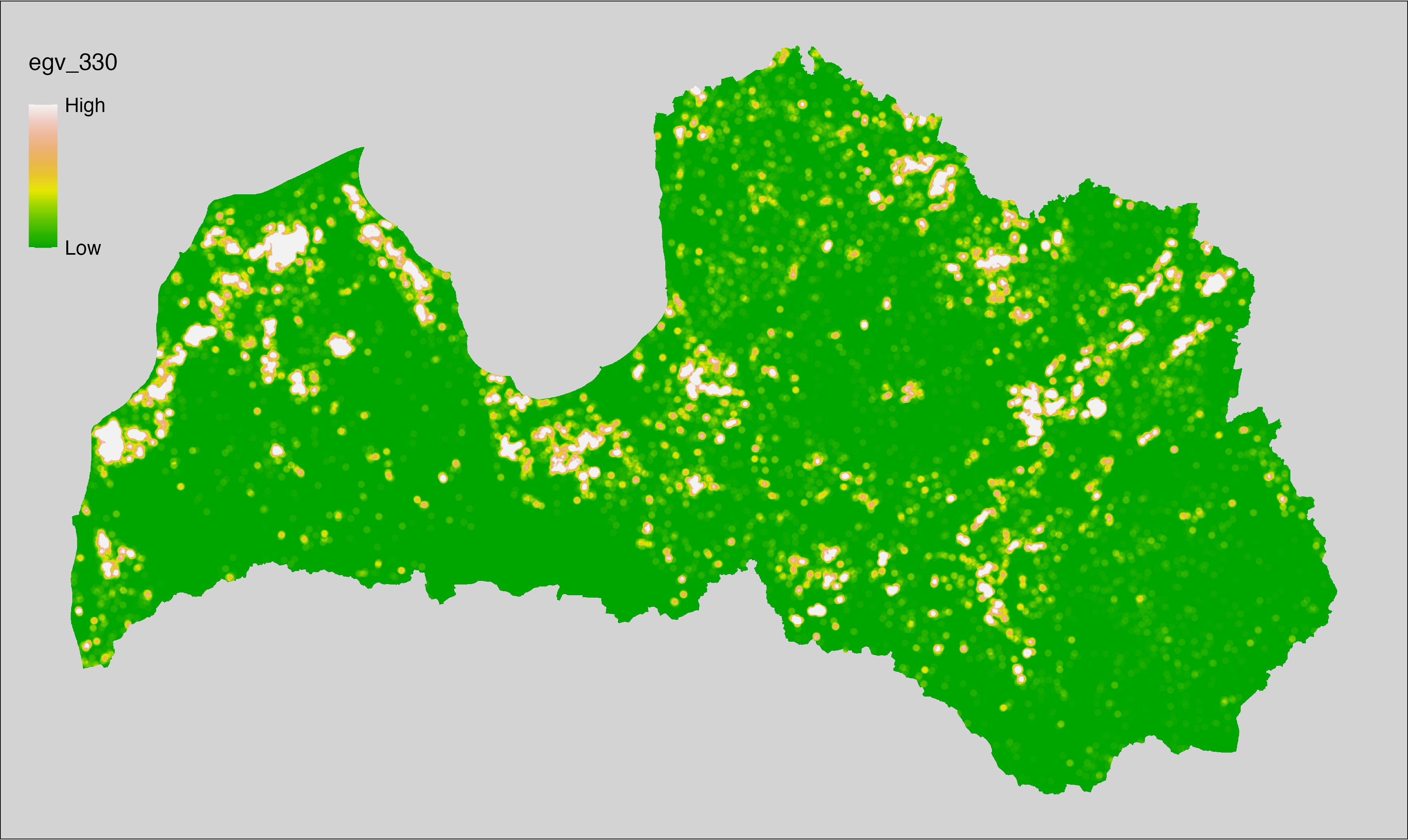
6.331 ForestsSoil_OligotrophicDrained_r3000
filename: ForestsSoil_OligotrophicDrained_r3000.tif
layername: egv_331
English name: Fractional cover of Drained Oligotrophic Forests within the 3 km landscape
Latvian name: Susinātu oligotrofu mežu platības īpatsvars 3 km ainavā
Procedure: The cover fraction within a radius of 3000 m around the analysis grid cell
is calculated as the area-weighted sum of the analysis cells inside
the buffer, using the workflow egvtools::radius_function(). During the calculation of the landscape
metric, inverse distance weighted (power = 2) gap filling on the output is
applied to ensure no missing values at the edges. Then the layer is
rewritten to set its name. Finally, the layer is standardised by
subtracting the arithmetic mean and dividing by the root mean squared error.
Code
# libs ----
if(!require(terra)) {install.packages("terra"); require(terra)}
if(!require(egvtools)) {remotes::install_github("aavotins/egvtools"); require(egvtools)}
# Templates -----
template100=rast("./Templates/TemplateRasters/LV100m_10km.tif")
# radii ----
radius_function(
kvadrati_path = "./Templates/TemplateGrids/tiles/",
radii_path = "./Templates/TemplateGridPoints/tiles/",
tikls100_path = "./Templates/TemplateGrids/tikls100_sauzeme.parquet",
template_path = "./Templates/TemplateRasters/LV100m_10km.tif",
input_layers = c("./RasterGrids_100m/2024/RAW/ForestsSoil_OligotrophicDrained_cell.tif"),
layer_prefixes = c("ForestsSoil_OligotrophicDrained"),
output_dir = "./RasterGrids_100m/2024/RAW/",
n_workers = 6,
radii = c("r3000"),
radius_mode = "sparse",
extract_fun = "mean",
fill_missing = TRUE,
IDW_weight = 2,
future_max_size = 40 * 1024^3)
# ForestsSoil_OligotrophicDrained_r3000.tif egv_331
slanis=rast("./RasterGrids_100m/2024/RAW/ForestsSoil_OligotrophicDrained_r3000.tif")
names(slanis)="egv_331"
slanis2=project(slanis,template100)
writeRaster(slanis2,
"./RasterGrids_100m/2024/RAW/ForestsSoil_OligotrophicDrained_r3000.tif",
overwrite=TRUE)
# standardisation ----
if(!require(terra)) {install.packages("terra"); require(terra)}
if(!require(tidyverse)) {install.packages("tidyverse"); require(tidyverse)}
nosaukums="ForestsSoil_OligotrophicDrained_r3000.tif"
ielasisanas_cels=paste0("./RasterGrids_100m/2024/RAW/",nosaukums)
saglabasanas_cels=paste0("./RasterGrids_100m/2024/Scaled/",nosaukums)
slanis=rast(ielasisanas_cels)
videjais=global(slanis,fun="mean",na.rm=TRUE)
centrets=slanis-videjais[,1]
standartnovirze=terra::global(centrets,fun="rms",na.rm=TRUE)
merogots=centrets/standartnovirze[,1]
writeRaster(merogots,
filename=saglabasanas_cels,
overwrite=TRUE)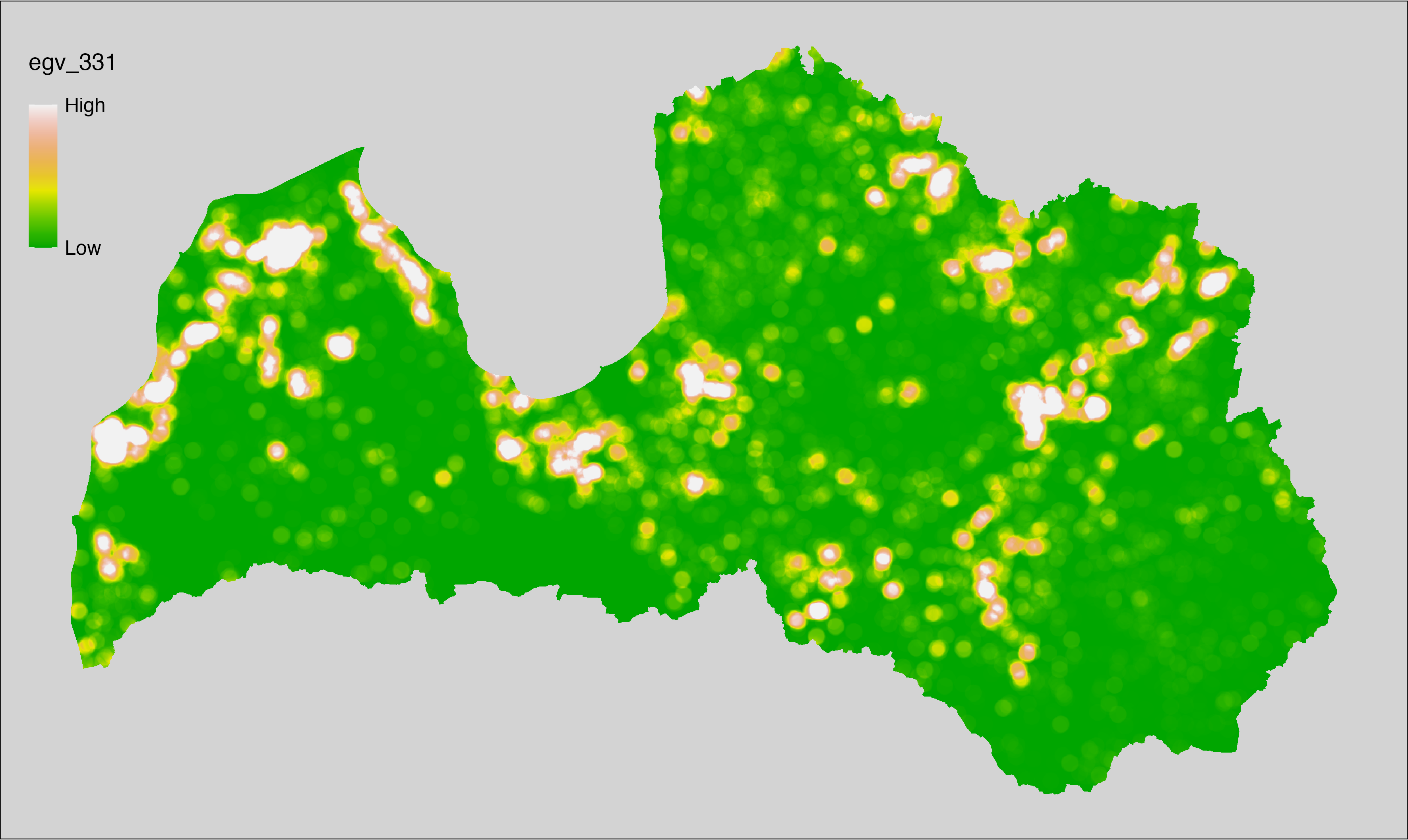
6.332 ForestsSoil_OligotrophicDrained_r10000
filename: ForestsSoil_OligotrophicDrained_r10000.tif
layername: egv_332
English name: Fractional cover of Drained Oligotrophic Forests within the 10 km landscape
Latvian name: Susinātu oligotrofu mežu platības īpatsvars 10 km ainavā
Procedure: The cover fraction within a radius of 10000 m around the analysis grid cell
is calculated as the area-weighted sum of the analysis cells inside
the buffer, using the workflow egvtools::radius_function(). During the calculation of the landscape
metric, inverse distance weighted (power = 2) gap filling on the output is
applied to ensure no missing values at the edges. Then the layer is
rewritten to set its name. Finally, the layer is standardised by
subtracting the arithmetic mean and dividing by the root mean squared error.
Code
# libs ----
if(!require(terra)) {install.packages("terra"); require(terra)}
if(!require(egvtools)) {remotes::install_github("aavotins/egvtools"); require(egvtools)}
# Templates -----
template100=rast("./Templates/TemplateRasters/LV100m_10km.tif")
# radii ----
radius_function(
kvadrati_path = "./Templates/TemplateGrids/tiles/",
radii_path = "./Templates/TemplateGridPoints/tiles/",
tikls100_path = "./Templates/TemplateGrids/tikls100_sauzeme.parquet",
template_path = "./Templates/TemplateRasters/LV100m_10km.tif",
input_layers = c("./RasterGrids_100m/2024/RAW/ForestsSoil_OligotrophicDrained_cell.tif"),
layer_prefixes = c("ForestsSoil_OligotrophicDrained"),
output_dir = "./RasterGrids_100m/2024/RAW/",
n_workers = 6,
radii = c("r10000"),
radius_mode = "sparse",
extract_fun = "mean",
fill_missing = TRUE,
IDW_weight = 2,
future_max_size = 40 * 1024^3)
# ForestsSoil_OligotrophicDrained_r10000.tif egv_332
slanis=rast("./RasterGrids_100m/2024/RAW/ForestsSoil_OligotrophicDrained_r10000.tif")
names(slanis)="egv_332"
slanis2=project(slanis,template100)
writeRaster(slanis2,
"./RasterGrids_100m/2024/RAW/ForestsSoil_OligotrophicDrained_r10000.tif",
overwrite=TRUE)
# standardisation ----
if(!require(terra)) {install.packages("terra"); require(terra)}
if(!require(tidyverse)) {install.packages("tidyverse"); require(tidyverse)}
nosaukums="ForestsSoil_OligotrophicDrained_r10000.tif"
ielasisanas_cels=paste0("./RasterGrids_100m/2024/RAW/",nosaukums)
saglabasanas_cels=paste0("./RasterGrids_100m/2024/Scaled/",nosaukums)
slanis=rast(ielasisanas_cels)
videjais=global(slanis,fun="mean",na.rm=TRUE)
centrets=slanis-videjais[,1]
standartnovirze=terra::global(centrets,fun="rms",na.rm=TRUE)
merogots=centrets/standartnovirze[,1]
writeRaster(merogots,
filename=saglabasanas_cels,
overwrite=TRUE)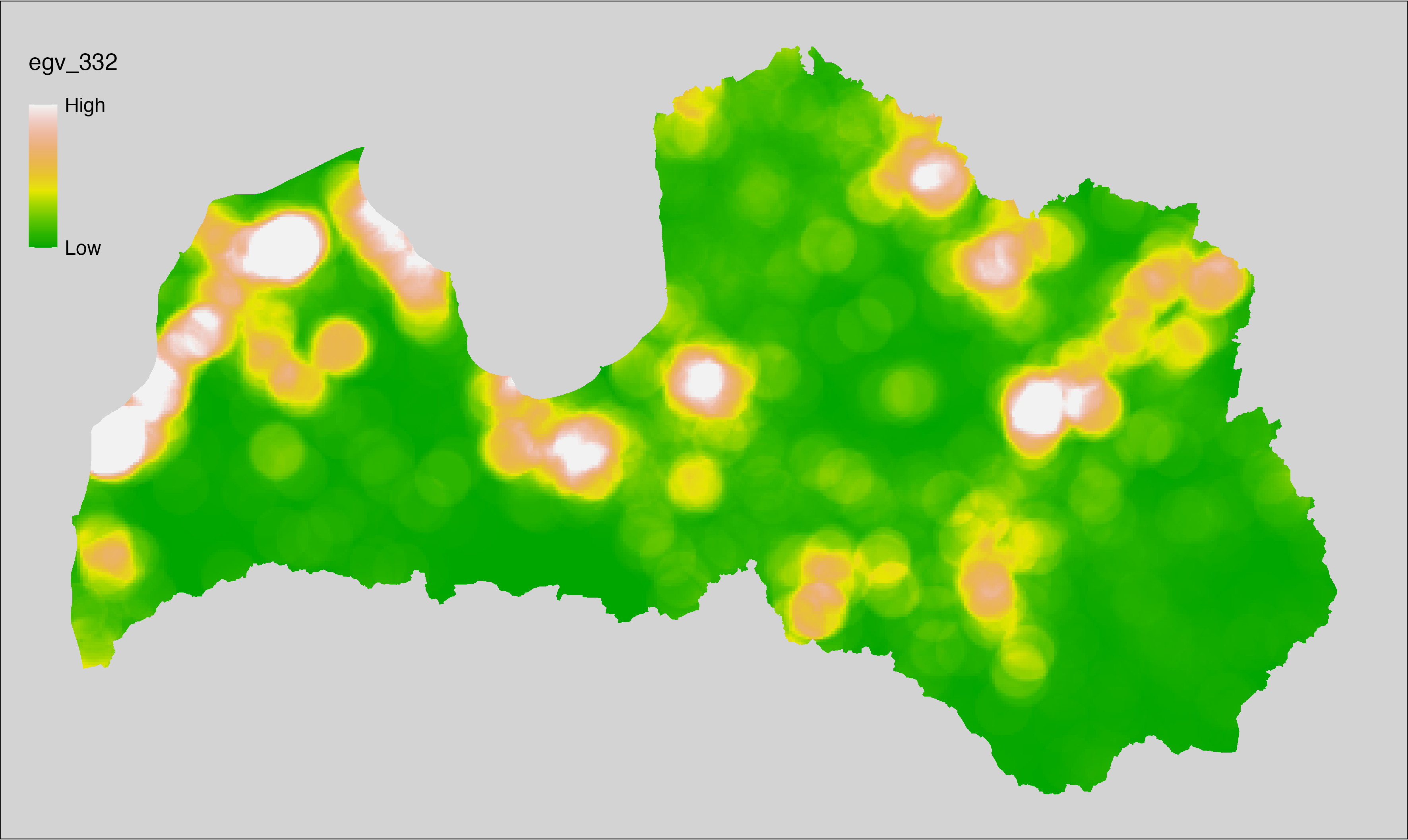
6.333 ForestsSoil_OligotrophicMineral_cell
filename: ForestsSoil_OligotrophicMineral_cell.tif
layername: egv_333
English name: Fractional cover of Oligotrophic Forests on undrained Mineral Soils within the analysis cell (1 ha)
Latvian name: Oligotrofu mežu nesusinātās minerālaugsnēs platības īpatsvars analīzes šūnā (1 ha)
Procedure: To prepare this EGV, forest stands with forest type equal to “1”,
“2”, “3”, “7” or “8” are selected from the State Forest Service’s State Forest
Registry and rasterised. Rasterisation is performed using the
workflow egvtools::polygon2input() with background
covering (value 0). The resulting layer
is then aggregated to EGV resolution using the workflow egvtools::input2egv(), which
calculates the arithmetic mean to determine the cover fraction. During
aggregation, inverse distance weighted (power = 2) gap filling on the output is
applied to ensure no missing values at the edges. Finally, the layer is
standardised by subtracting the arithmetic mean and dividing by the root mean squared
error.
Code
# libs ----
if(!require(egvtools)) {remotes::install_github("aavotins/egvtools"); require(egvtools)}
if(!require(terra)) {install.packages("terra"); require(terra)}
if(!require(sf)) {install.packages("sf"); require(sf)}
if(!require(tidyverse)) {install.packages("tidyverse"); require(tidyverse)}
if(!require(sfarrow)) {install.packages("sfarrow"); require(sfarrow)}
if(!require(readxl)) {install.packages("readxl"); require(readxl)}
if(!require(raster)) {install.packages("raster"); require(raster)}
if(!require(fasterize)) {install.packages("fasterize"); require(fasterize)}
# templates ----
template100=rast("./Templates/TemplateRasters/LV100m_10km.tif")
template10=rast("./Templates/TemplateRasters/LV10m_10km.tif")
rastrs10=raster(template10)
nulls10=rast("./Templates/TemplateRasters/nulls_LV10m_10km.tif")
nulls100=rast("./Templates/TemplateRasters/nulls_LV100m_10km.tif")
# simple landscape ----
simple_landscape=rast("RasterGrids_10m/2024/Ainava_vienk_mask.tif")
# mvr ----
mvr=st_read_parquet("./Geodata/2024/MVR/nogabali_2024janv.parquet")
mvr$yes=1
# ForestsSoil_OligotrophicMineral_cell.tif egv_333 ----
OligotrophicMineral=mvr %>%
filter(mt %in% c("1","2","3","7","8"))
p2i_rez=egvtools::polygon2input(vector_data = OligotrophicMineral,
template_path = "./Templates/TemplateRasters/LV10m_10km.tif",
out_path = "./RasterGrids_10m/2024/",
file_name = "ForestsSoil_OligotrophicMineral_input.tif",
value_field = "yes",
prepare=FALSE,
background_raster = "./Templates/TemplateRasters/nulls_LV10m_10km.tif",
plot_result = TRUE)
p2i_rez
i2e_rez=egvtools::input2egv(input=paste0("./RasterGrids_10m/2024/",
"ForestsSoil_OligotrophicMineral_input.tif"),
egv_template= "./Templates/TemplateRasters/LV100m_10km.tif",
summary_function = "average",
missing_job = "FillOutput",
outlocation = "./RasterGrids_100m/2024/RAW/",
outfilename = "ForestsSoil_OligotrophicMineral_cell.tif",
layername = "egv_333",
idw_weight = 2,
plot_gaps = FALSE,plot_final = TRUE)
i2e_rez
rm(OligotrophicMineral)
rm(p2i_rez)
rm(i2e_rez)
unlink("./RasterGrids_10m/2024/ForestsSoil_OligotrophicMineral_input.tif")
# standardisation ----
if(!require(terra)) {install.packages("terra"); require(terra)}
if(!require(tidyverse)) {install.packages("tidyverse"); require(tidyverse)}
nosaukums="ForestsSoil_OligotrophicMineral_cell.tif"
ielasisanas_cels=paste0("./RasterGrids_100m/2024/RAW/",nosaukums)
saglabasanas_cels=paste0("./RasterGrids_100m/2024/Scaled/",nosaukums)
slanis=rast(ielasisanas_cels)
videjais=global(slanis,fun="mean",na.rm=TRUE)
centrets=slanis-videjais[,1]
standartnovirze=terra::global(centrets,fun="rms",na.rm=TRUE)
merogots=centrets/standartnovirze[,1]
writeRaster(merogots,
filename=saglabasanas_cels,
overwrite=TRUE)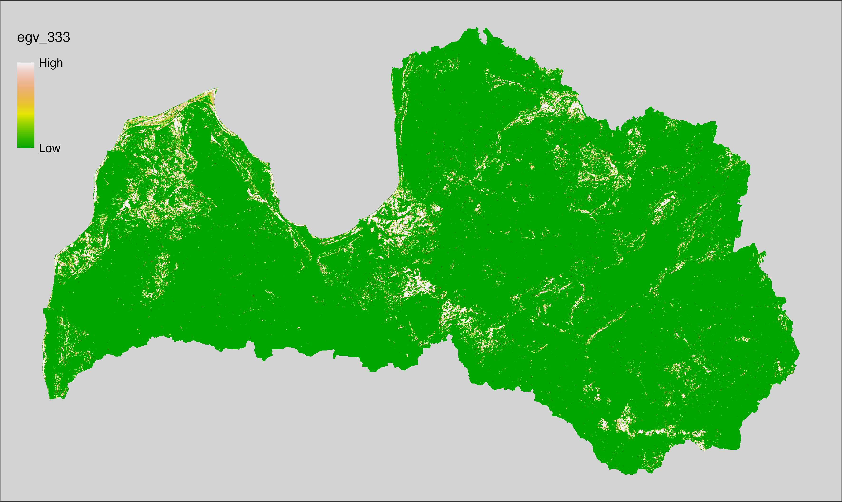
6.334 ForestsSoil_OligotrophicMineral_r500
filename: ForestsSoil_OligotrophicMineral_r500.tif
layername: egv_334
English name: Fractional cover of Oligotrophic Forests on undrained Mineral Soils within the 0.5 km landscape
Latvian name: Oligotrofu mežu nesusinātās minerālaugsnēs platības īpatsvars 0,5 km ainavā
Procedure: The cover fraction within a radius of 500 m around the analysis grid cell is
calculated as the area-weighted sum of the analysis cells inside the
buffer, using the workflow egvtools::radius_function(). During the calculation of the landscape metric,
inverse distance weighted (power = 2) gap filling on the output is applied
to ensure no missing values at the edges. Then the layer is rewritten to set
its name. Finally, the layer is standardised by subtracting the arithmetic
mean and dividing by the root mean squared error.
Code
# libs ----
if(!require(terra)) {install.packages("terra"); require(terra)}
if(!require(egvtools)) {remotes::install_github("aavotins/egvtools"); require(egvtools)}
# Templates -----
template100=rast("./Templates/TemplateRasters/LV100m_10km.tif")
# radii ----
radius_function(
kvadrati_path = "./Templates/TemplateGrids/tiles/",
radii_path = "./Templates/TemplateGridPoints/tiles/",
tikls100_path = "./Templates/TemplateGrids/tikls100_sauzeme.parquet",
template_path = "./Templates/TemplateRasters/LV100m_10km.tif",
input_layers = c("./RasterGrids_100m/2024/RAW/ForestsSoil_OligotrophicMineral_cell.tif"),
layer_prefixes = c("ForestsSoil_OligotrophicMineral"),
output_dir = "./RasterGrids_100m/2024/RAW/",
n_workers = 6,
radii = c("r500"),
radius_mode = "sparse",
extract_fun = "mean",
fill_missing = TRUE,
IDW_weight = 2,
future_max_size = 40 * 1024^3)
# ForestsSoil_OligotrophicMineral_r500.tif egv_334
slanis=rast("./RasterGrids_100m/2024/RAW/ForestsSoil_OligotrophicMineral_r500.tif")
names(slanis)="egv_334"
slanis2=project(slanis,template100)
writeRaster(slanis2,
"./RasterGrids_100m/2024/RAW/ForestsSoil_OligotrophicMineral_r500.tif",
overwrite=TRUE)
# standardisation ----
if(!require(terra)) {install.packages("terra"); require(terra)}
if(!require(tidyverse)) {install.packages("tidyverse"); require(tidyverse)}
nosaukums="ForestsSoil_OligotrophicMineral_r500.tif"
ielasisanas_cels=paste0("./RasterGrids_100m/2024/RAW/",nosaukums)
saglabasanas_cels=paste0("./RasterGrids_100m/2024/Scaled/",nosaukums)
slanis=rast(ielasisanas_cels)
videjais=global(slanis,fun="mean",na.rm=TRUE)
centrets=slanis-videjais[,1]
standartnovirze=terra::global(centrets,fun="rms",na.rm=TRUE)
merogots=centrets/standartnovirze[,1]
writeRaster(merogots,
filename=saglabasanas_cels,
overwrite=TRUE)
6.335 ForestsSoil_OligotrophicMineral_r1250
filename: ForestsSoil_OligotrophicMineral_r1250.tif
layername: egv_335
English name: Fractional cover of Oligotrophic Forests on undrained Mineral Soils within the 1.25 km landscape
Latvian name: Oligotrofu mežu nesusinātās minerālaugsnēs platības īpatsvars 1,25 km ainavā
Procedure: The cover fraction within a radius of 1250 m around the analysis grid cell
is calculated as the area-weighted sum of the analysis cells inside
the buffer, using the workflow egvtools::radius_function(). During the calculation of the landscape
metric, inverse distance weighted (power = 2) gap filling on the output is
applied to ensure no missing values at the edges. Then the layer is
rewritten to set its name. Finally, the layer is standardised by
subtracting the arithmetic mean and dividing by the root mean squared error.
Code
# libs ----
if(!require(terra)) {install.packages("terra"); require(terra)}
if(!require(egvtools)) {remotes::install_github("aavotins/egvtools"); require(egvtools)}
# Templates -----
template100=rast("./Templates/TemplateRasters/LV100m_10km.tif")
# radii ----
radius_function(
kvadrati_path = "./Templates/TemplateGrids/tiles/",
radii_path = "./Templates/TemplateGridPoints/tiles/",
tikls100_path = "./Templates/TemplateGrids/tikls100_sauzeme.parquet",
template_path = "./Templates/TemplateRasters/LV100m_10km.tif",
input_layers = c("./RasterGrids_100m/2024/RAW/ForestsSoil_OligotrophicMineral_cell.tif"),
layer_prefixes = c("ForestsSoil_OligotrophicMineral"),
output_dir = "./RasterGrids_100m/2024/RAW/",
n_workers = 6,
radii = c("r1250"),
radius_mode = "sparse",
extract_fun = "mean",
fill_missing = TRUE,
IDW_weight = 2,
future_max_size = 40 * 1024^3)
# ForestsSoil_OligotrophicMineral_r1250.tif egv_335
slanis=rast("./RasterGrids_100m/2024/RAW/ForestsSoil_OligotrophicMineral_r1250.tif")
names(slanis)="egv_335"
slanis2=project(slanis,template100)
writeRaster(slanis2,
"./RasterGrids_100m/2024/RAW/ForestsSoil_OligotrophicMineral_r1250.tif",
overwrite=TRUE)
# standardisation ----
if(!require(terra)) {install.packages("terra"); require(terra)}
if(!require(tidyverse)) {install.packages("tidyverse"); require(tidyverse)}
nosaukums="ForestsSoil_OligotrophicMineral_r1250.tif"
ielasisanas_cels=paste0("./RasterGrids_100m/2024/RAW/",nosaukums)
saglabasanas_cels=paste0("./RasterGrids_100m/2024/Scaled/",nosaukums)
slanis=rast(ielasisanas_cels)
videjais=global(slanis,fun="mean",na.rm=TRUE)
centrets=slanis-videjais[,1]
standartnovirze=terra::global(centrets,fun="rms",na.rm=TRUE)
merogots=centrets/standartnovirze[,1]
writeRaster(merogots,
filename=saglabasanas_cels,
overwrite=TRUE)
6.336 ForestsSoil_OligotrophicMineral_r3000
filename: ForestsSoil_OligotrophicMineral_r3000.tif
layername: egv_336
English name: Fractional cover of Oligotrophic Forests on undrained Mineral Soils within the 3 km landscape
Latvian name: Oligotrofu mežu nesusinātās minerālaugsnēs platības īpatsvars 3 km ainavā
Procedure: The cover fraction within a radius of 3000 m around the analysis grid cell
is calculated as the area-weighted sum of the analysis cells inside
the buffer, using the workflow egvtools::radius_function(). During the calculation of the landscape
metric, inverse distance weighted (power = 2) gap filling on the output is
applied to ensure no missing values at the edges. Then the layer is
rewritten to set its name. Finally, the layer is standardised by
subtracting the arithmetic mean and dividing by the root mean squared error.
Code
# libs ----
if(!require(terra)) {install.packages("terra"); require(terra)}
if(!require(egvtools)) {remotes::install_github("aavotins/egvtools"); require(egvtools)}
# Templates -----
template100=rast("./Templates/TemplateRasters/LV100m_10km.tif")
# radii ----
radius_function(
kvadrati_path = "./Templates/TemplateGrids/tiles/",
radii_path = "./Templates/TemplateGridPoints/tiles/",
tikls100_path = "./Templates/TemplateGrids/tikls100_sauzeme.parquet",
template_path = "./Templates/TemplateRasters/LV100m_10km.tif",
input_layers = c("./RasterGrids_100m/2024/RAW/ForestsSoil_OligotrophicMineral_cell.tif"),
layer_prefixes = c("ForestsSoil_OligotrophicMineral"),
output_dir = "./RasterGrids_100m/2024/RAW/",
n_workers = 6,
radii = c("r3000"),
radius_mode = "sparse",
extract_fun = "mean",
fill_missing = TRUE,
IDW_weight = 2,
future_max_size = 40 * 1024^3)
# ForestsSoil_OligotrophicMineral_r3000.tif egv_336
slanis=rast("./RasterGrids_100m/2024/RAW/ForestsSoil_OligotrophicMineral_r3000.tif")
names(slanis)="egv_336"
slanis2=project(slanis,template100)
writeRaster(slanis2,
"./RasterGrids_100m/2024/RAW/ForestsSoil_OligotrophicMineral_r3000.tif",
overwrite=TRUE)
# standardisation ----
if(!require(terra)) {install.packages("terra"); require(terra)}
if(!require(tidyverse)) {install.packages("tidyverse"); require(tidyverse)}
nosaukums="ForestsSoil_OligotrophicMineral_r3000.tif"
ielasisanas_cels=paste0("./RasterGrids_100m/2024/RAW/",nosaukums)
saglabasanas_cels=paste0("./RasterGrids_100m/2024/Scaled/",nosaukums)
slanis=rast(ielasisanas_cels)
videjais=global(slanis,fun="mean",na.rm=TRUE)
centrets=slanis-videjais[,1]
standartnovirze=terra::global(centrets,fun="rms",na.rm=TRUE)
merogots=centrets/standartnovirze[,1]
writeRaster(merogots,
filename=saglabasanas_cels,
overwrite=TRUE)
6.337 ForestsSoil_OligotrophicMineral_r10000
filename: ForestsSoil_OligotrophicMineral_r10000.tif
layername: egv_337
English name: Fractional cover of Oligotrophic Forests on undrained Mineral Soils within the 10 km landscape
Latvian name: Oligotrofu mežu nesusinātās minerālaugsnēs platības īpatsvars 10 km ainavā
Procedure: The cover fraction within a radius of 10000 m around the analysis grid cell
is calculated as the area-weighted sum of the analysis cells inside
the buffer, using the workflow egvtools::radius_function(). During the calculation of the landscape
metric, inverse distance weighted (power = 2) gap filling on the output is
applied to ensure no missing values at the edges. Then the layer is
rewritten to set its name. Finally, the layer is standardised by
subtracting the arithmetic mean and dividing by the root mean squared error.
Code
# libs ----
if(!require(terra)) {install.packages("terra"); require(terra)}
if(!require(egvtools)) {remotes::install_github("aavotins/egvtools"); require(egvtools)}
# Templates -----
template100=rast("./Templates/TemplateRasters/LV100m_10km.tif")
# radii ----
radius_function(
kvadrati_path = "./Templates/TemplateGrids/tiles/",
radii_path = "./Templates/TemplateGridPoints/tiles/",
tikls100_path = "./Templates/TemplateGrids/tikls100_sauzeme.parquet",
template_path = "./Templates/TemplateRasters/LV100m_10km.tif",
input_layers = c("./RasterGrids_100m/2024/RAW/ForestsSoil_OligotrophicMineral_cell.tif"),
layer_prefixes = c("ForestsSoil_OligotrophicMineral"),
output_dir = "./RasterGrids_100m/2024/RAW/",
n_workers = 6,
radii = c("r10000"),
radius_mode = "sparse",
extract_fun = "mean",
fill_missing = TRUE,
IDW_weight = 2,
future_max_size = 40 * 1024^3)
# ForestsSoil_OligotrophicMineral_r10000.tif egv_337
slanis=rast("./RasterGrids_100m/2024/RAW/ForestsSoil_OligotrophicMineral_r10000.tif")
names(slanis)="egv_337"
slanis2=project(slanis,template100)
writeRaster(slanis2,
"./RasterGrids_100m/2024/RAW/ForestsSoil_OligotrophicMineral_r10000.tif",
overwrite=TRUE)
# standardisation ----
if(!require(terra)) {install.packages("terra"); require(terra)}
if(!require(tidyverse)) {install.packages("tidyverse"); require(tidyverse)}
nosaukums="ForestsSoil_OligotrophicMineral_r10000.tif"
ielasisanas_cels=paste0("./RasterGrids_100m/2024/RAW/",nosaukums)
saglabasanas_cels=paste0("./RasterGrids_100m/2024/Scaled/",nosaukums)
slanis=rast(ielasisanas_cels)
videjais=global(slanis,fun="mean",na.rm=TRUE)
centrets=slanis-videjais[,1]
standartnovirze=terra::global(centrets,fun="rms",na.rm=TRUE)
merogots=centrets/standartnovirze[,1]
writeRaster(merogots,
filename=saglabasanas_cels,
overwrite=TRUE)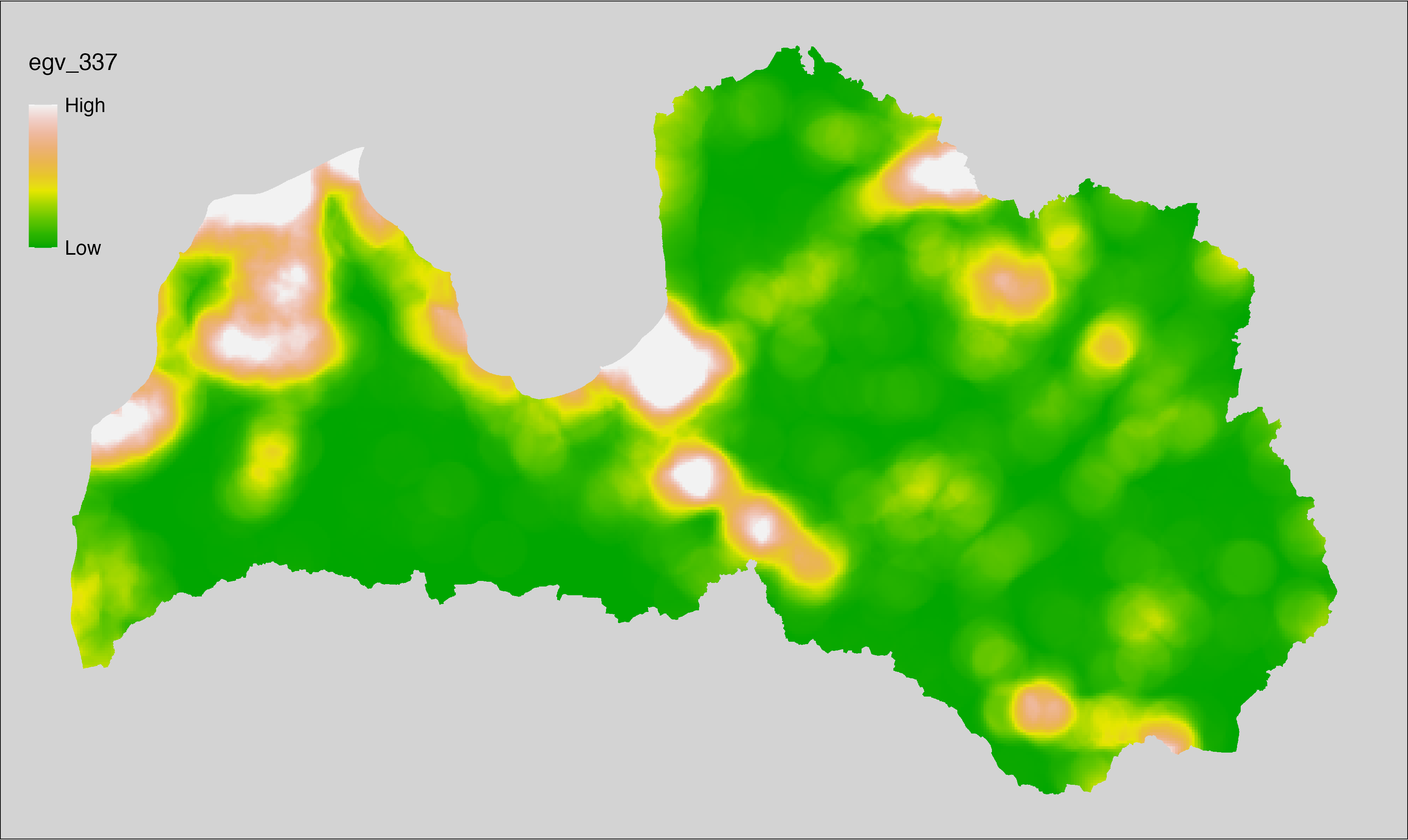
6.338 ForestsSoil_OligotrophicOrganic_cell
filename: ForestsSoil_OligotrophicOrganic_cell.tif
layername: egv_338
English name: Fractional cover of Oligotrophic Forests on undrained Organic Soils within the analysis cell (1 ha)
Latvian name: Oligotrofu mežu nesusinātās organiskajās augsnēs platības īpatsvars analīzes šūnā (1 ha)
Procedure: To prepare this EGV, forest stands with forest type equal to “12”
or “14” are selected from the State Forest Service’s State Forest
Registry and rasterised. Rasterisation is performed using
the workflow egvtools::polygon2input() with background
covering (value 0). The resulting layer
is then aggregated to EGV resolution using the workflow egvtools::input2egv(), which
calculates the arithmetic mean to determine the cover fraction. During
aggregation, inverse distance weighted (power = 2) gap filling on the output is
applied to ensure no missing values at the edges. Finally, the layer is
standardised by subtracting the arithmetic mean and dividing by the root mean squared
error.
Code
# libs ----
if(!require(egvtools)) {remotes::install_github("aavotins/egvtools"); require(egvtools)}
if(!require(terra)) {install.packages("terra"); require(terra)}
if(!require(sf)) {install.packages("sf"); require(sf)}
if(!require(tidyverse)) {install.packages("tidyverse"); require(tidyverse)}
if(!require(sfarrow)) {install.packages("sfarrow"); require(sfarrow)}
if(!require(readxl)) {install.packages("readxl"); require(readxl)}
if(!require(raster)) {install.packages("raster"); require(raster)}
if(!require(fasterize)) {install.packages("fasterize"); require(fasterize)}
# templates ----
template100=rast("./Templates/TemplateRasters/LV100m_10km.tif")
template10=rast("./Templates/TemplateRasters/LV10m_10km.tif")
rastrs10=raster(template10)
nulls10=rast("./Templates/TemplateRasters/nulls_LV10m_10km.tif")
nulls100=rast("./Templates/TemplateRasters/nulls_LV100m_10km.tif")
# simple landscape ----
simple_landscape=rast("RasterGrids_10m/2024/Ainava_vienk_mask.tif")
# mvr ----
mvr=st_read_parquet("./Geodata/2024/MVR/nogabali_2024janv.parquet")
mvr$yes=1
# ForestsSoil_OligotrophicOrganic_cell.tif egv_338 ----
OligotrophicOrganic=mvr %>%
filter(mt %in% c("12","14"))
p2i_rez=egvtools::polygon2input(vector_data = OligotrophicOrganic,
template_path = "./Templates/TemplateRasters/LV10m_10km.tif",
out_path = "./RasterGrids_10m/2024/",
file_name = "ForestsSoil_OligotrophicOrganic_input.tif",
value_field = "yes",
prepare=FALSE,
background_raster = "./Templates/TemplateRasters/nulls_LV10m_10km.tif",
plot_result = TRUE)
p2i_rez
i2e_rez=egvtools::input2egv(input=paste0("./RasterGrids_10m/2024/",
"ForestsSoil_OligotrophicOrganic_input.tif"),
egv_template= "./Templates/TemplateRasters/LV100m_10km.tif",
summary_function = "average",
missing_job = "FillOutput",
outlocation = "./RasterGrids_100m/2024/RAW/",
outfilename = "ForestsSoil_OligotrophicOrganic_cell.tif",
layername = "egv_338",
idw_weight = 2,
plot_gaps = FALSE,plot_final = TRUE)
i2e_rez
rm(OligotrophicOrganic)
rm(p2i_rez)
rm(i2e_rez)
unlink("./RasterGrids_10m/2024/ForestsSoil_OligotrophicOrganic_input.tif")
# standardisation ----
if(!require(terra)) {install.packages("terra"); require(terra)}
if(!require(tidyverse)) {install.packages("tidyverse"); require(tidyverse)}
nosaukums="ForestsSoil_OligotrophicMineral_cell.tif"
ielasisanas_cels=paste0("./RasterGrids_100m/2024/RAW/",nosaukums)
saglabasanas_cels=paste0("./RasterGrids_100m/2024/Scaled/",nosaukums)
slanis=rast(ielasisanas_cels)
videjais=global(slanis,fun="mean",na.rm=TRUE)
centrets=slanis-videjais[,1]
standartnovirze=terra::global(centrets,fun="rms",na.rm=TRUE)
merogots=centrets/standartnovirze[,1]
writeRaster(merogots,
filename=saglabasanas_cels,
overwrite=TRUE)
6.339 ForestsSoil_OligotrophicOrganic_r500
filename: ForestsSoil_OligotrophicOrganic_r500.tif
layername: egv_339
English name: Fractional cover of Oligotrophic Forests on undrained Organic Soils within the 0.5 km landscape
Latvian name: Oligotrofu mežu nesusinātās organiskajās augsnēs platības īpatsvars 0,5 km ainavā
Procedure: The cover fraction within a radius of 500 m around the analysis grid cell is
calculated as the area-weighted sum of the analysis cells inside the
buffer, using the workflow egvtools::radius_function(). During the calculation of the landscape metric,
inverse distance weighted (power = 2) gap filling on the output is applied
to ensure no missing values at the edges. Then the layer is rewritten to set
its name. Finally, the layer is standardised by subtracting the arithmetic
mean and dividing by the root mean squared error.
Code
# libs ----
if(!require(terra)) {install.packages("terra"); require(terra)}
if(!require(egvtools)) {remotes::install_github("aavotins/egvtools"); require(egvtools)}
# Templates -----
template100=rast("./Templates/TemplateRasters/LV100m_10km.tif")
# radii ----
radius_function(
kvadrati_path = "./Templates/TemplateGrids/tiles/",
radii_path = "./Templates/TemplateGridPoints/tiles/",
tikls100_path = "./Templates/TemplateGrids/tikls100_sauzeme.parquet",
template_path = "./Templates/TemplateRasters/LV100m_10km.tif",
input_layers = c("./RasterGrids_100m/2024/RAW/ForestsSoil_OligotrophicOrganic_cell.tif"),
layer_prefixes = c("ForestsSoil_OligotrophicOrganic"),
output_dir = "./RasterGrids_100m/2024/RAW/",
n_workers = 6,
radii = c("r500"),
radius_mode = "sparse",
extract_fun = "mean",
fill_missing = TRUE,
IDW_weight = 2,
future_max_size = 40 * 1024^3)
# ForestsSoil_OligotrophicOrganic_r500.tif egv_339
slanis=rast("./RasterGrids_100m/2024/RAW/ForestsSoil_OligotrophicOrganic_r500.tif")
names(slanis)="egv_339"
slanis2=project(slanis,template100)
writeRaster(slanis2,
"./RasterGrids_100m/2024/RAW/ForestsSoil_OligotrophicOrganic_r500.tif",
overwrite=TRUE)
# standardisation ----
if(!require(terra)) {install.packages("terra"); require(terra)}
if(!require(tidyverse)) {install.packages("tidyverse"); require(tidyverse)}
nosaukums="ForestsSoil_OligotrophicOrganic_r500.tif"
ielasisanas_cels=paste0("./RasterGrids_100m/2024/RAW/",nosaukums)
saglabasanas_cels=paste0("./RasterGrids_100m/2024/Scaled/",nosaukums)
slanis=rast(ielasisanas_cels)
videjais=global(slanis,fun="mean",na.rm=TRUE)
centrets=slanis-videjais[,1]
standartnovirze=terra::global(centrets,fun="rms",na.rm=TRUE)
merogots=centrets/standartnovirze[,1]
writeRaster(merogots,
filename=saglabasanas_cels,
overwrite=TRUE)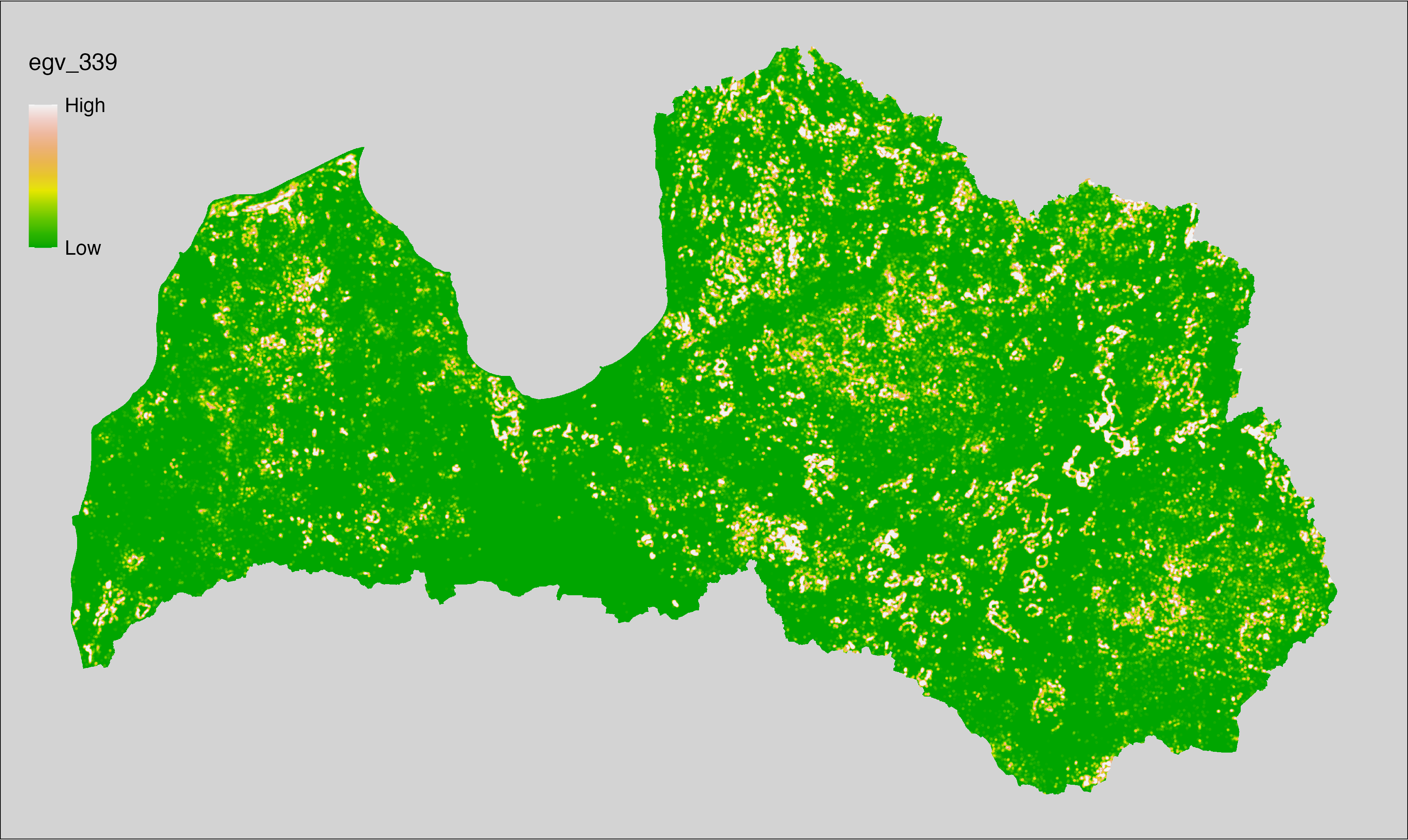
6.340 ForestsSoil_OligotrophicOrganic_r1250
filename: ForestsSoil_OligotrophicOrganic_r1250.tif
layername: egv_340
English name: Fractional cover of Oligotrophic Forests on undrained Organic Soils within the 1.25 km landscape
Latvian name: Oligotrofu mežu nesusinātās organiskajās augsnēs platības īpatsvars 1,25 km ainavā
Procedure: The cover fraction within a radius of 1250 m around the analysis grid cell
is calculated as the area-weighted sum of the analysis cells inside
the buffer, using the workflow egvtools::radius_function(). During the calculation of the landscape
metric, inverse distance weighted (power = 2) gap filling on the output is
applied to ensure no missing values at the edges. Then the layer is
rewritten to set its name. Finally, the layer is standardised by
subtracting the arithmetic mean and dividing by the root mean squared error.
Code
# libs ----
if(!require(terra)) {install.packages("terra"); require(terra)}
if(!require(egvtools)) {remotes::install_github("aavotins/egvtools"); require(egvtools)}
# Templates -----
template100=rast("./Templates/TemplateRasters/LV100m_10km.tif")
# radii ----
radius_function(
kvadrati_path = "./Templates/TemplateGrids/tiles/",
radii_path = "./Templates/TemplateGridPoints/tiles/",
tikls100_path = "./Templates/TemplateGrids/tikls100_sauzeme.parquet",
template_path = "./Templates/TemplateRasters/LV100m_10km.tif",
input_layers = c("./RasterGrids_100m/2024/RAW/ForestsSoil_OligotrophicOrganic_cell.tif"),
layer_prefixes = c("ForestsSoil_OligotrophicOrganic"),
output_dir = "./RasterGrids_100m/2024/RAW/",
n_workers = 6,
radii = c("r1250"),
radius_mode = "sparse",
extract_fun = "mean",
fill_missing = TRUE,
IDW_weight = 2,
future_max_size = 40 * 1024^3)
# ForestsSoil_OligotrophicOrganic_r1250.tif egv_340
slanis=rast("./RasterGrids_100m/2024/RAW/ForestsSoil_OligotrophicOrganic_r1250.tif")
names(slanis)="egv_340"
slanis2=project(slanis,template100)
writeRaster(slanis2,
"./RasterGrids_100m/2024/RAW/ForestsSoil_OligotrophicOrganic_r1250.tif",
overwrite=TRUE)
# standardisation ----
if(!require(terra)) {install.packages("terra"); require(terra)}
if(!require(tidyverse)) {install.packages("tidyverse"); require(tidyverse)}
nosaukums="ForestsSoil_OligotrophicOrganic_r1250.tif"
ielasisanas_cels=paste0("./RasterGrids_100m/2024/RAW/",nosaukums)
saglabasanas_cels=paste0("./RasterGrids_100m/2024/Scaled/",nosaukums)
slanis=rast(ielasisanas_cels)
videjais=global(slanis,fun="mean",na.rm=TRUE)
centrets=slanis-videjais[,1]
standartnovirze=terra::global(centrets,fun="rms",na.rm=TRUE)
merogots=centrets/standartnovirze[,1]
writeRaster(merogots,
filename=saglabasanas_cels,
overwrite=TRUE)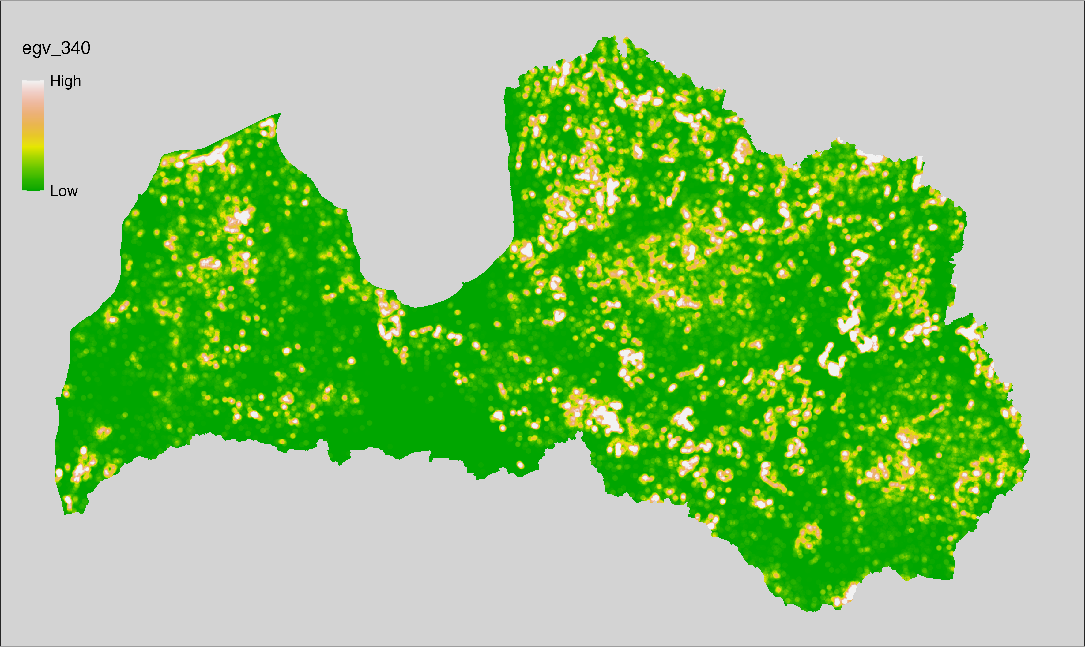
6.341 ForestsSoil_OligotrophicOrganic_r3000
filename: ForestsSoil_OligotrophicOrganic_r3000.tif
layername: egv_341
English name: Fractional cover of Oligotrophic Forests on undrained Organic Soils within the 3 km landscape
Latvian name: Oligotrofu mežu nesusinātās organiskajās augsnēs platības īpatsvars 3 km ainavā
Procedure: The cover fraction within a radius of 3000 m around the analysis grid cell
is calculated as the area-weighted sum of the analysis cells inside
the buffer, using the workflow egvtools::radius_function(). During the calculation of the landscape
metric, inverse distance weighted (power = 2) gap filling on the output is
applied to ensure no missing values at the edges. Then the layer is
rewritten to set its name. Finally, the layer is standardised by
subtracting the arithmetic mean and dividing by the root mean squared error.
Code
# libs ----
if(!require(terra)) {install.packages("terra"); require(terra)}
if(!require(egvtools)) {remotes::install_github("aavotins/egvtools"); require(egvtools)}
# Templates -----
template100=rast("./Templates/TemplateRasters/LV100m_10km.tif")
# radii ----
radius_function(
kvadrati_path = "./Templates/TemplateGrids/tiles/",
radii_path = "./Templates/TemplateGridPoints/tiles/",
tikls100_path = "./Templates/TemplateGrids/tikls100_sauzeme.parquet",
template_path = "./Templates/TemplateRasters/LV100m_10km.tif",
input_layers = c("./RasterGrids_100m/2024/RAW/ForestsSoil_OligotrophicOrganic_cell.tif"),
layer_prefixes = c("ForestsSoil_OligotrophicOrganic"),
output_dir = "./RasterGrids_100m/2024/RAW/",
n_workers = 6,
radii = c("r3000"),
radius_mode = "sparse",
extract_fun = "mean",
fill_missing = TRUE,
IDW_weight = 2,
future_max_size = 40 * 1024^3)
# ForestsSoil_OligotrophicOrganic_r3000.tif egv_341
slanis=rast("./RasterGrids_100m/2024/RAW/ForestsSoil_OligotrophicOrganic_r3000.tif")
names(slanis)="egv_341"
slanis2=project(slanis,template100)
writeRaster(slanis2,
"./RasterGrids_100m/2024/RAW/ForestsSoil_OligotrophicOrganic_r3000.tif",
overwrite=TRUE)
# standardisation ----
if(!require(terra)) {install.packages("terra"); require(terra)}
if(!require(tidyverse)) {install.packages("tidyverse"); require(tidyverse)}
nosaukums="ForestsSoil_OligotrophicOrganic_r3000.tif"
ielasisanas_cels=paste0("./RasterGrids_100m/2024/RAW/",nosaukums)
saglabasanas_cels=paste0("./RasterGrids_100m/2024/Scaled/",nosaukums)
slanis=rast(ielasisanas_cels)
videjais=global(slanis,fun="mean",na.rm=TRUE)
centrets=slanis-videjais[,1]
standartnovirze=terra::global(centrets,fun="rms",na.rm=TRUE)
merogots=centrets/standartnovirze[,1]
writeRaster(merogots,
filename=saglabasanas_cels,
overwrite=TRUE)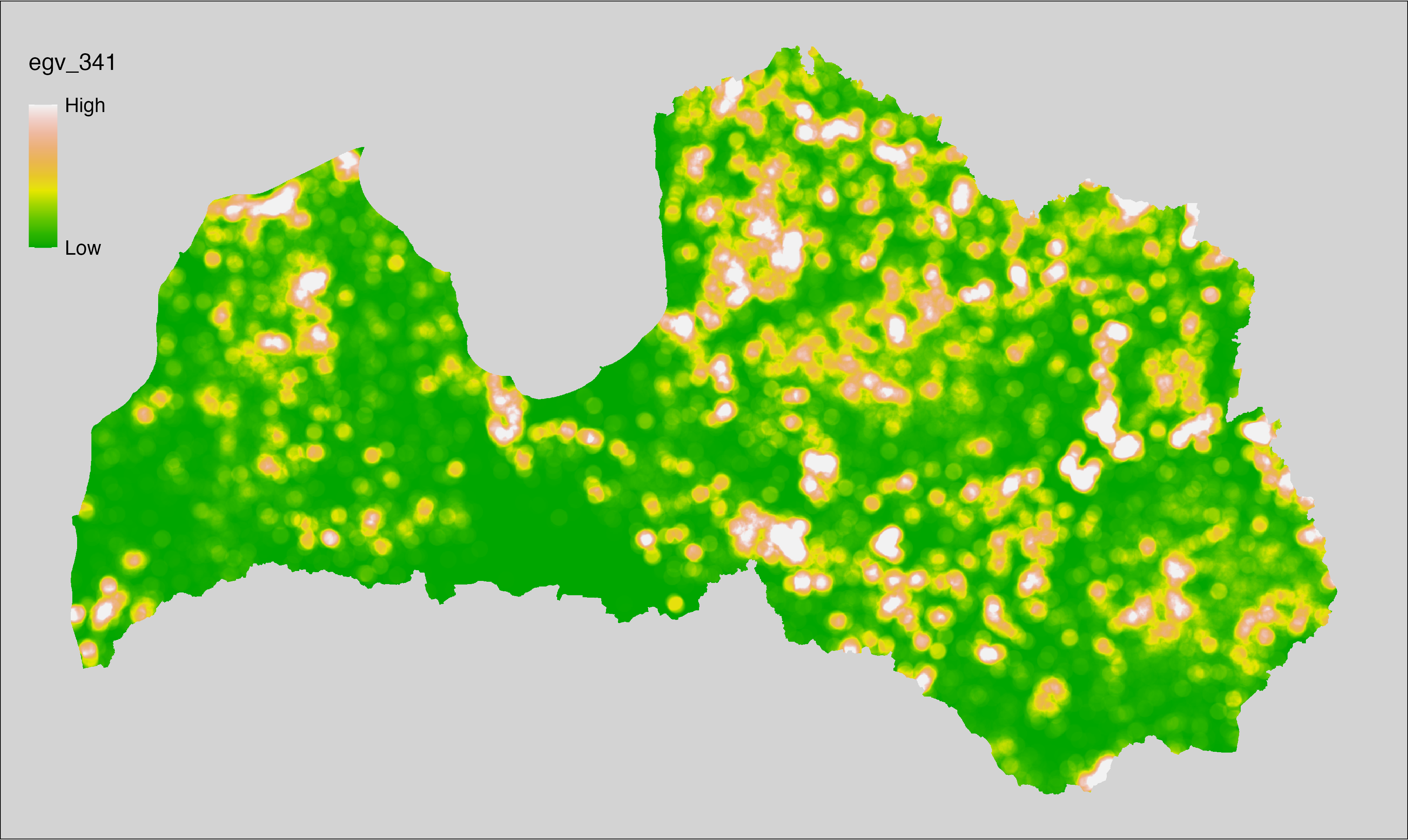
6.342 ForestsSoil_OligotrophicOrganic_r10000
filename: ForestsSoil_OligotrophicOrganic_r10000.tif
layername: egv_342
English name: Fractional cover of Oligotrophic Forests on undrained Organic Soils within the 10 km landscape
Latvian name: Oligotrofu mežu nesusinātās organiskajās augsnēs platības īpatsvars 10 km ainavā
Procedure: The cover fraction within a radius of 10000 m around the analysis grid cell
is calculated as the area-weighted sum of the analysis cells inside
the buffer, using the workflow egvtools::radius_function(). During the calculation of the landscape
metric, inverse distance weighted (power = 2) gap filling on the output is
applied to ensure no missing values at the edges. Then the layer is
rewritten to set its name. Finally, the layer is standardised by
subtracting the arithmetic mean and dividing by the root mean squared error.
Code
# libs ----
if(!require(terra)) {install.packages("terra"); require(terra)}
if(!require(egvtools)) {remotes::install_github("aavotins/egvtools"); require(egvtools)}
# Templates -----
template100=rast("./Templates/TemplateRasters/LV100m_10km.tif")
# radii ----
radius_function(
kvadrati_path = "./Templates/TemplateGrids/tiles/",
radii_path = "./Templates/TemplateGridPoints/tiles/",
tikls100_path = "./Templates/TemplateGrids/tikls100_sauzeme.parquet",
template_path = "./Templates/TemplateRasters/LV100m_10km.tif",
input_layers = c("./RasterGrids_100m/2024/RAW/ForestsSoil_OligotrophicOrganic_cell.tif"),
layer_prefixes = c("ForestsSoil_OligotrophicOrganic"),
output_dir = "./RasterGrids_100m/2024/RAW/",
n_workers = 6,
radii = c("r10000"),
radius_mode = "sparse",
extract_fun = "mean",
fill_missing = TRUE,
IDW_weight = 2,
future_max_size = 40 * 1024^3)
# ForestsSoil_OligotrophicOrganic_r10000.tif egv_342
slanis=rast("./RasterGrids_100m/2024/RAW/ForestsSoil_OligotrophicOrganic_r10000.tif")
names(slanis)="egv_342"
slanis2=project(slanis,template100)
writeRaster(slanis2,
"./RasterGrids_100m/2024/RAW/ForestsSoil_OligotrophicOrganic_r10000.tif",
overwrite=TRUE)
# standardisation ----
if(!require(terra)) {install.packages("terra"); require(terra)}
if(!require(tidyverse)) {install.packages("tidyverse"); require(tidyverse)}
nosaukums="ForestsSoil_OligotrophicOrganic_r10000.tif"
ielasisanas_cels=paste0("./RasterGrids_100m/2024/RAW/",nosaukums)
saglabasanas_cels=paste0("./RasterGrids_100m/2024/Scaled/",nosaukums)
slanis=rast(ielasisanas_cels)
videjais=global(slanis,fun="mean",na.rm=TRUE)
centrets=slanis-videjais[,1]
standartnovirze=terra::global(centrets,fun="rms",na.rm=TRUE)
merogots=centrets/standartnovirze[,1]
writeRaster(merogots,
filename=saglabasanas_cels,
overwrite=TRUE)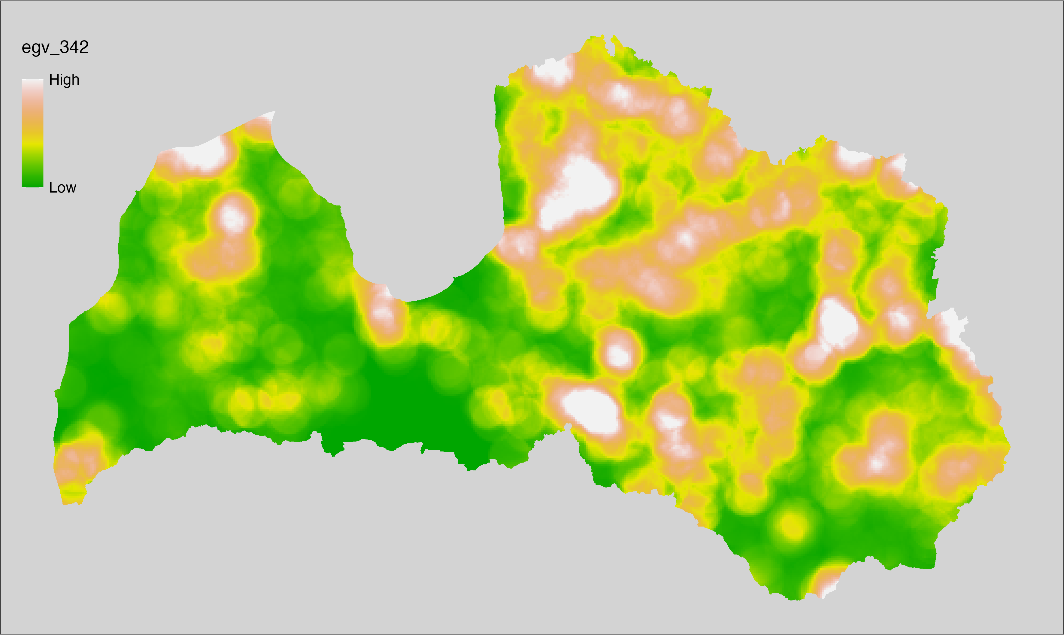
6.343 ForestsTreesAge_BorealDeciduousOld_cell
filename: ForestsTreesAge_BorealDeciduousOld_cell.tif
layername: egv_343
English name: Fractional cover of Old (over rotation age) Boreal Deciduous Forests within the analysis cell (1 ha)
Latvian name: Vecu (kopš cirtmeta) šaurlapju mežu platības īpatsvars analīzes šūnā (1 ha)
Procedure: Most EGVs describing forests are spatially restricted to areas outside of clearcuts and dead stands. This mask is created using a combination of the State Forest Service’s State Forest Registry land category 12 and 14, and The Global Forest Watch pixels classified as lost tree canopy cover since 2020 (raster layer matching input, presence = 1, absence = 0).
To prepare this EGV, stands from the State Forest Service’s State Forest Registry are classified into (in order):
coniferous (see Terminology and acronyms for species codes) if timber volume of those species exceeded 75%;
Boreal deciduous if timber volume of those species exceeded 75%;
temperate deciduous if timber volume of those species exceeded 50%;
mixed otherwise;
then Boreal deciduous stands exceeding the legal rotation age are selected and
geometries are rasterised (presence = 1, NA otherwise). Rasterisation is
performed using the workflow egvtools::polygon2input(), restricting to pixels outside clearcut
mask and covering background with value 0. The resulting layer
is then aggregated to EGV resolution using the workflow egvtools::input2egv(), which
calculates the arithmetic mean to determine the cover fraction. During
aggregation, inverse distance weighted (power = 2) gap filling on the output is
applied to ensure no missing values at the edges. Finally, the layer is
standardised by subtracting the arithmetic mean and dividing by the root mean squared
error.
Code
# libs ----
if(!require(egvtools)) {remotes::install_github("aavotins/egvtools"); require(egvtools)}
if(!require(terra)) {install.packages("terra"); require(terra)}
if(!require(sf)) {install.packages("sf"); require(sf)}
if(!require(tidyverse)) {install.packages("tidyverse"); require(tidyverse)}
if(!require(sfarrow)) {install.packages("sfarrow"); require(sfarrow)}
if(!require(readxl)) {install.packages("readxl"); require(readxl)}
if(!require(raster)) {install.packages("raster"); require(raster)}
if(!require(fasterize)) {install.packages("fasterize"); require(fasterize)}
# templates ----
template100=rast("./Templates/TemplateRasters/LV100m_10km.tif")
template10=rast("./Templates/TemplateRasters/LV10m_10km.tif")
rastrs10=raster(template10)
nulls10=rast("./Templates/TemplateRasters/nulls_LV10m_10km.tif")
nulls100=rast("./Templates/TemplateRasters/nulls_LV100m_10km.tif")
# simple landscape ----
simple_landscape=rast("RasterGrids_10m/2024/Ainava_vienk_mask.tif")
# mvr ----
mvr=st_read_parquet("./Geodata/2024/MVR/nogabali_2024janv.parquet")
mvr$yes=1
# clear cut mask ----
izcirtumi=mvr %>%
filter(zkat %in% c("12","14")) %>%
dplyr::select(yes)
r_izcirtumi_mvr=fasterize(izcirtumi,rastrs10,field="yes")
t_izcirtumi_mvr=rast(r_izcirtumi_mvr)
plot(t_izcirtumi_mvr)
tcl=rast("./Geodata/2024/Trees/GFW/TreeCoverLoss_v1_12.tif")
tcl2=ifel(tcl<20,0,1)
tclX=cover(tcl2,nulls10)
plot(tclX)
clearcut_mask=cover(t_izcirtumi_mvr,tclX,
filename="./RasterGrids_10m/2024/Mask_clearcuts.tif",
overwrite=TRUE)
plot(clearcut_mask)
rm(izcirtumi)
rm(r_izcirtumi_mvr)
rm(t_izcirtumi_mvr)
rm(tcl)
rm(tcl2)
rm(tclX)
# ForestsTreesAge_BorealDeciduousOld_cell.tif egv_343 ----
skujkoki=c("1","3","13","14","15","22","23","28") # 8
saurlapji=c("4","6","8","9","19","20","21","32","35","68") # 10
platlapji=c("10","11","12","16","17","18","24","25","26","27","28","29","50",
"61","62","63","64","65","66","67","69") # 21
mvr=mvr %>%
mutate(kraja_skujkoku=ifelse(s10 %in% skujkoki,v10,0)+
ifelse(s11 %in% skujkoki,v11,0)+ifelse(s12 %in% skujkoki,v12,0)+
ifelse(s13 %in% skujkoki,v13,0)+ifelse(s14 %in% skujkoki,v14,0),
kraja_saurlapju=ifelse(s10 %in% saurlapji,v10,0)+
ifelse(s11 %in% saurlapji,v11,0)+ifelse(s12 %in% saurlapji,v12,0)+
ifelse(s13 %in% saurlapji,v13,0)+ifelse(s14 %in% saurlapji,v14,0),
kraja_platlapju=ifelse(s10 %in% platlapji,v10,0)+
ifelse(s11 %in% platlapji,v11,0)+ifelse(s12 %in% platlapji,v12,0)+
ifelse(s13 %in% platlapji,v13,0)+ifelse(s14 %in% platlapji,v14,0)) %>%
mutate(kopeja_kraja=kraja_skujkoku+kraja_platlapju+kraja_saurlapju) %>%
mutate(tips=ifelse(kraja_skujkoku/kopeja_kraja>=0.75,"skujkoku",
ifelse(kraja_saurlapju/kopeja_kraja>=0.75,"saurlapju",
ifelse(kraja_platlapju/kopeja_kraja>0.5,"platlapju",
"jauktu koku"))))
nogabali=mvr %>%
filter(zkat=="10"&tips=="saurlapju"&(vgr=="4"|vgr=="5"))
p2i_rez=egvtools::polygon2input(vector_data = nogabali,
template_path = "./Templates/TemplateRasters/LV10m_10km.tif",
out_path = "./RasterGrids_10m/2024/",
file_name = "ForestsTreesAge_BorealDeciduousOld_input.tif",
value_field = "yes",
restrict_to = clearcut_mask,
restrict_values = 0,
prepare=FALSE,
background_raster = "./Templates/TemplateRasters/nulls_LV10m_10km.tif",
plot_result = TRUE)
p2i_rez
i2e_rez=egvtools::input2egv(input=paste0("./RasterGrids_10m/2024/",
"ForestsTreesAge_BorealDeciduousOld_input.tif"),
egv_template= "./Templates/TemplateRasters/LV100m_10km.tif",
summary_function = "average",
missing_job = "FillOutput",
outlocation = "./RasterGrids_100m/2024/RAW/",
outfilename = "ForestsTreesAge_BorealDeciduousOld_cell.tif",
layername = "egv_343",
idw_weight = 2,
plot_gaps = FALSE,plot_final = TRUE)
i2e_rez
rm(nogabali)
rm(p2i_rez)
rm(i2e_rez)
unlink("./RasterGrids_10m/2024/ForestsTreesAge_BorealDeciduousOld_input.tif")
# standardisation ----
if(!require(terra)) {install.packages("terra"); require(terra)}
if(!require(tidyverse)) {install.packages("tidyverse"); require(tidyverse)}
nosaukums="ForestsTreesAge_BorealDeciduousOld_cell.tif"
ielasisanas_cels=paste0("./RasterGrids_100m/2024/RAW/",nosaukums)
saglabasanas_cels=paste0("./RasterGrids_100m/2024/Scaled/",nosaukums)
slanis=rast(ielasisanas_cels)
videjais=global(slanis,fun="mean",na.rm=TRUE)
centrets=slanis-videjais[,1]
standartnovirze=terra::global(centrets,fun="rms",na.rm=TRUE)
merogots=centrets/standartnovirze[,1]
writeRaster(merogots,
filename=saglabasanas_cels,
overwrite=TRUE)
6.344 ForestsTreesAge_BorealDeciduousOld_r500
filename: ForestsTreesAge_BorealDeciduousOld_r500.tif
layername: egv_344
English name: Fractional cover of Old (over rotation age) Boreal Deciduous Forests within the 0.5 km landscape
Latvian name: Vecu (kopš cirtmeta) šaurlapju mežu platības īpatsvars 0,5 km ainavā
Procedure: The cover fraction within a radius of 500 m around the analysis grid cell is
calculated as the area-weighted sum of the analysis cells inside the
buffer, using the workflow egvtools::radius_function(). During the calculation of the landscape metric,
inverse distance weighted (power = 2) gap filling on the output is applied
to ensure no missing values at the edges. Then the layer is rewritten to set
its name. Finally, the layer is standardised by subtracting the arithmetic
mean and dividing by the root mean squared error.
Code
# libs ----
if(!require(terra)) {install.packages("terra"); require(terra)}
if(!require(egvtools)) {remotes::install_github("aavotins/egvtools"); require(egvtools)}
# Templates -----
template100=rast("./Templates/TemplateRasters/LV100m_10km.tif")
# radii ----
radius_function(
kvadrati_path = "./Templates/TemplateGrids/tiles/",
radii_path = "./Templates/TemplateGridPoints/tiles/",
tikls100_path = "./Templates/TemplateGrids/tikls100_sauzeme.parquet",
template_path = "./Templates/TemplateRasters/LV100m_10km.tif",
input_layers = c("./RasterGrids_100m/2024/RAW/ForestsTreesAge_BorealDeciduousOld_cell.tif"),
layer_prefixes = c("ForestsTreesAge_BorealDeciduousOld"),
output_dir = "./RasterGrids_100m/2024/RAW/",
n_workers = 6,
radii = c("r500"),
radius_mode = "sparse",
extract_fun = "mean",
fill_missing = TRUE,
IDW_weight = 2,
future_max_size = 40 * 1024^3)
# ForestsTreesAge_BorealDeciduousOld_r500.tif egv_344
slanis=rast("./RasterGrids_100m/2024/RAW/ForestsTreesAge_BorealDeciduousOld_r500.tif")
names(slanis)="egv_344"
slanis2=project(slanis,template100)
writeRaster(slanis2,
"./RasterGrids_100m/2024/RAW/ForestsTreesAge_BorealDeciduousOld_r500.tif",
overwrite=TRUE)
# standardisation ----
if(!require(terra)) {install.packages("terra"); require(terra)}
if(!require(tidyverse)) {install.packages("tidyverse"); require(tidyverse)}
nosaukums="ForestsTreesAge_BorealDeciduousOld_r500.tif"
ielasisanas_cels=paste0("./RasterGrids_100m/2024/RAW/",nosaukums)
saglabasanas_cels=paste0("./RasterGrids_100m/2024/Scaled/",nosaukums)
slanis=rast(ielasisanas_cels)
videjais=global(slanis,fun="mean",na.rm=TRUE)
centrets=slanis-videjais[,1]
standartnovirze=terra::global(centrets,fun="rms",na.rm=TRUE)
merogots=centrets/standartnovirze[,1]
writeRaster(merogots,
filename=saglabasanas_cels,
overwrite=TRUE)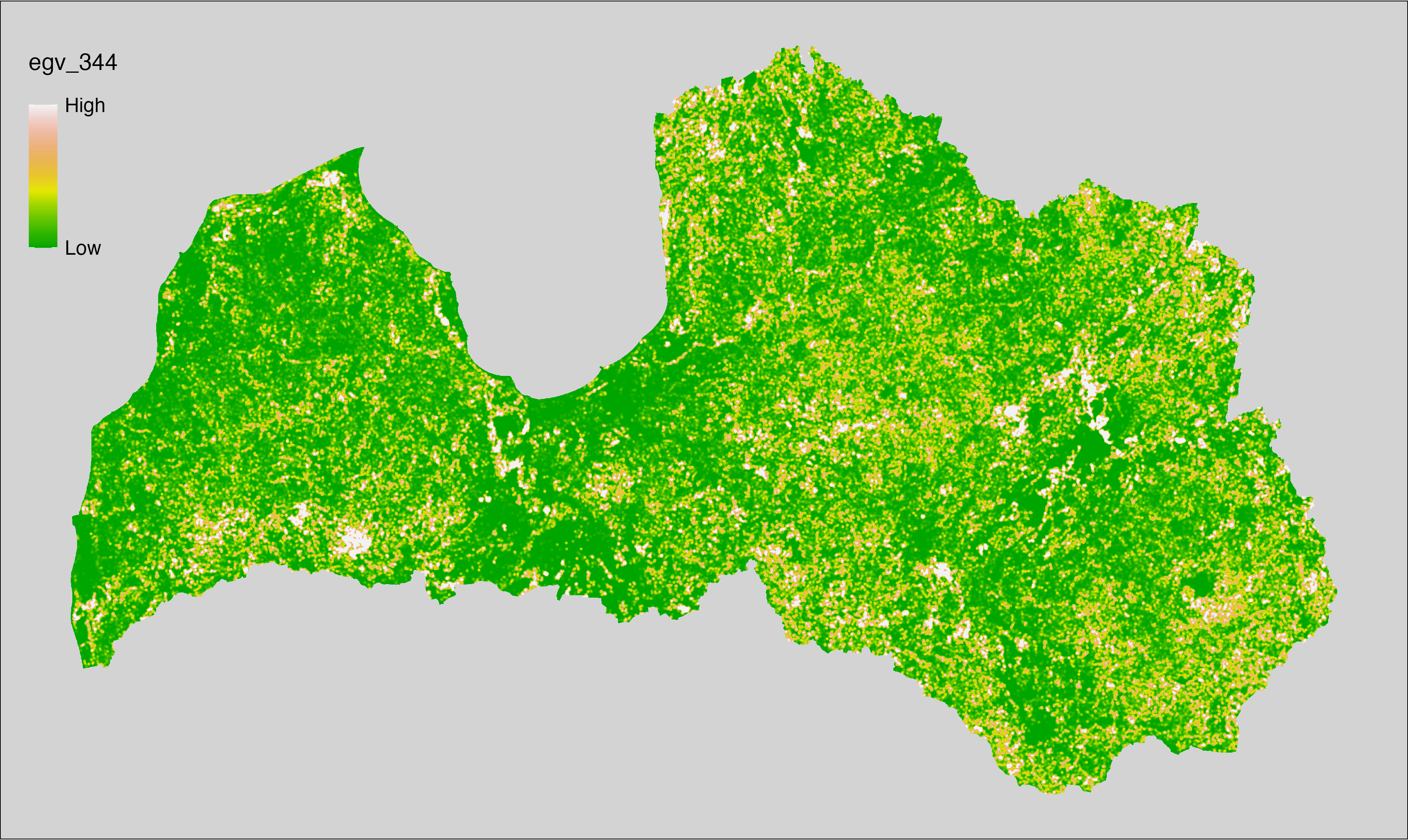
6.345 ForestsTreesAge_BorealDeciduousOld_r1250
filename: ForestsTreesAge_BorealDeciduousOld_r1250.tif
layername: egv_345
English name: Fractional cover of Old (over rotation age) Boreal Deciduous Forests within the 1.25 km landscape
Latvian name: Vecu (kopš cirtmeta) šaurlapju mežu platības īpatsvars 1,25 km ainavā
Procedure: The cover fraction within a radius of 1250 m around the analysis grid cell
is calculated as the area-weighted sum of the analysis cells inside
the buffer, using the workflow egvtools::radius_function(). During the calculation of the landscape
metric, inverse distance weighted (power = 2) gap filling on the output is
applied to ensure no missing values at the edges. Then the layer is
rewritten to set its name. Finally, the layer is standardised by
subtracting the arithmetic mean and dividing by the root mean squared error.
Code
# libs ----
if(!require(terra)) {install.packages("terra"); require(terra)}
if(!require(egvtools)) {remotes::install_github("aavotins/egvtools"); require(egvtools)}
# Templates -----
template100=rast("./Templates/TemplateRasters/LV100m_10km.tif")
# radii ----
radius_function(
kvadrati_path = "./Templates/TemplateGrids/tiles/",
radii_path = "./Templates/TemplateGridPoints/tiles/",
tikls100_path = "./Templates/TemplateGrids/tikls100_sauzeme.parquet",
template_path = "./Templates/TemplateRasters/LV100m_10km.tif",
input_layers = c("./RasterGrids_100m/2024/RAW/ForestsTreesAge_BorealDeciduousOld_cell.tif"),
layer_prefixes = c("ForestsTreesAge_BorealDeciduousOld"),
output_dir = "./RasterGrids_100m/2024/RAW/",
n_workers = 6,
radii = c("r1250"),
radius_mode = "sparse",
extract_fun = "mean",
fill_missing = TRUE,
IDW_weight = 2,
future_max_size = 40 * 1024^3)
# ForestsTreesAge_BorealDeciduousOld_r1250.tif egv_345
slanis=rast("./RasterGrids_100m/2024/RAW/ForestsTreesAge_BorealDeciduousOld_r1250.tif")
names(slanis)="egv_345"
slanis2=project(slanis,template100)
writeRaster(slanis2,
"./RasterGrids_100m/2024/RAW/ForestsTreesAge_BorealDeciduousOld_r1250.tif",
overwrite=TRUE)
# standardisation ----
if(!require(terra)) {install.packages("terra"); require(terra)}
if(!require(tidyverse)) {install.packages("tidyverse"); require(tidyverse)}
nosaukums="ForestsTreesAge_BorealDeciduousOld_r1250.tif"
ielasisanas_cels=paste0("./RasterGrids_100m/2024/RAW/",nosaukums)
saglabasanas_cels=paste0("./RasterGrids_100m/2024/Scaled/",nosaukums)
slanis=rast(ielasisanas_cels)
videjais=global(slanis,fun="mean",na.rm=TRUE)
centrets=slanis-videjais[,1]
standartnovirze=terra::global(centrets,fun="rms",na.rm=TRUE)
merogots=centrets/standartnovirze[,1]
writeRaster(merogots,
filename=saglabasanas_cels,
overwrite=TRUE)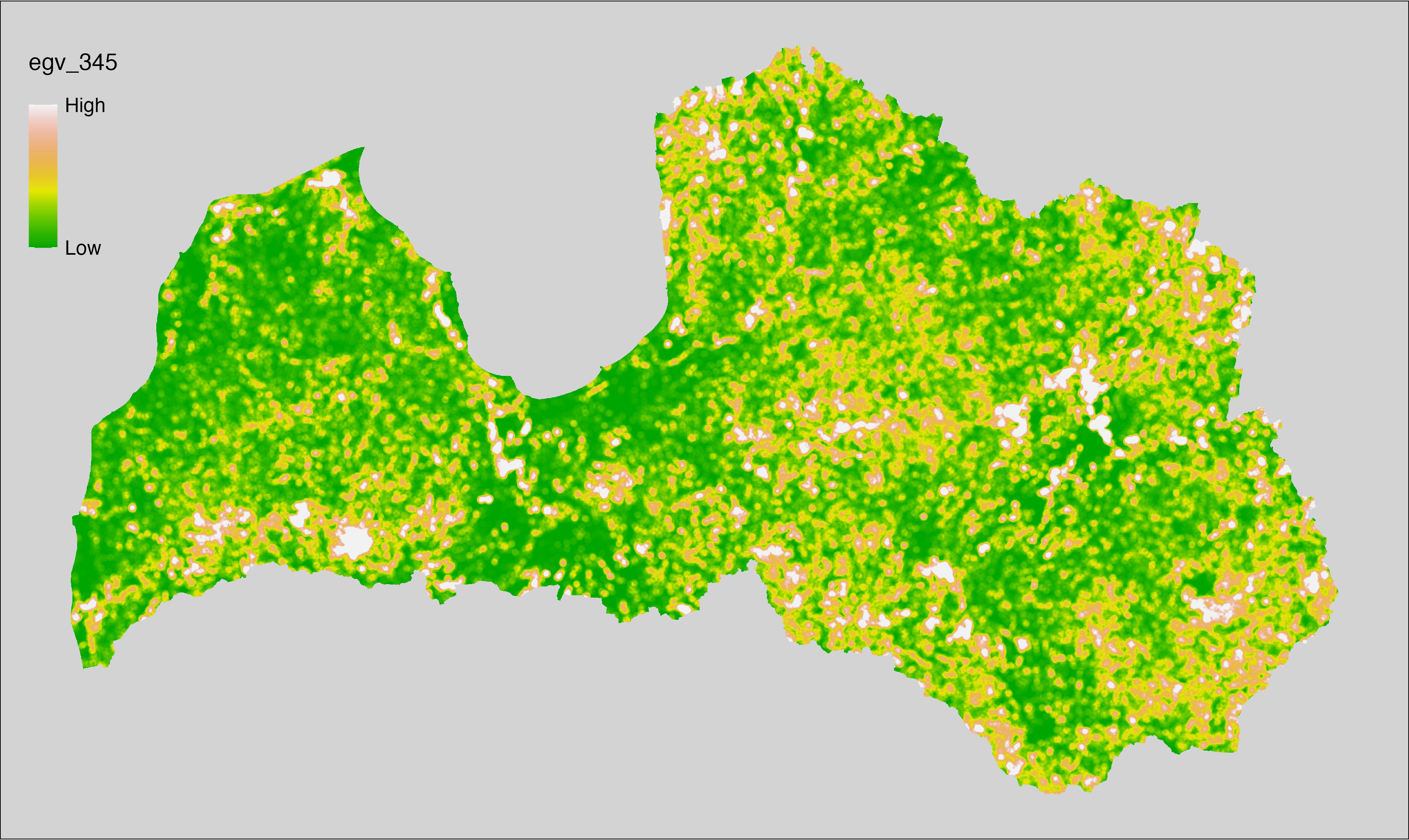
6.346 ForestsTreesAge_BorealDeciduousOld_r3000
filename: ForestsTreesAge_BorealDeciduousOld_r3000.tif
layername: egv_346
English name: Fractional cover of Old (over rotation age) Boreal Deciduous Forests within the 3 km landscape
Latvian name: Vecu (kopš cirtmeta) šaurlapju mežu platības īpatsvars 3 km ainavā
Procedure: The cover fraction within a radius of 3000 m around the analysis grid cell
is calculated as the area-weighted sum of the analysis cells inside
the buffer, using the workflow egvtools::radius_function(). During the calculation of the landscape
metric, inverse distance weighted (power = 2) gap filling on the output is
applied to ensure no missing values at the edges. Then the layer is
rewritten to set its name. Finally, the layer is standardised by
subtracting the arithmetic mean and dividing by the root mean squared error.
Code
# libs ----
if(!require(terra)) {install.packages("terra"); require(terra)}
if(!require(egvtools)) {remotes::install_github("aavotins/egvtools"); require(egvtools)}
# Templates -----
template100=rast("./Templates/TemplateRasters/LV100m_10km.tif")
# radii ----
radius_function(
kvadrati_path = "./Templates/TemplateGrids/tiles/",
radii_path = "./Templates/TemplateGridPoints/tiles/",
tikls100_path = "./Templates/TemplateGrids/tikls100_sauzeme.parquet",
template_path = "./Templates/TemplateRasters/LV100m_10km.tif",
input_layers = c("./RasterGrids_100m/2024/RAW/ForestsTreesAge_BorealDeciduousOld_cell.tif"),
layer_prefixes = c("ForestsTreesAge_BorealDeciduousOld"),
output_dir = "./RasterGrids_100m/2024/RAW/",
n_workers = 6,
radii = c("r3000"),
radius_mode = "sparse",
extract_fun = "mean",
fill_missing = TRUE,
IDW_weight = 2,
future_max_size = 40 * 1024^3)
# ForestsTreesAge_BorealDeciduousOld_r3000.tif egv_346
slanis=rast("./RasterGrids_100m/2024/RAW/ForestsTreesAge_BorealDeciduousOld_r3000.tif")
names(slanis)="egv_346"
slanis2=project(slanis,template100)
writeRaster(slanis2,
"./RasterGrids_100m/2024/RAW/ForestsTreesAge_BorealDeciduousOld_r3000.tif",
overwrite=TRUE)
# standardisation ----
if(!require(terra)) {install.packages("terra"); require(terra)}
if(!require(tidyverse)) {install.packages("tidyverse"); require(tidyverse)}
nosaukums="ForestsTreesAge_BorealDeciduousOld_r3000.tif"
ielasisanas_cels=paste0("./RasterGrids_100m/2024/RAW/",nosaukums)
saglabasanas_cels=paste0("./RasterGrids_100m/2024/Scaled/",nosaukums)
slanis=rast(ielasisanas_cels)
videjais=global(slanis,fun="mean",na.rm=TRUE)
centrets=slanis-videjais[,1]
standartnovirze=terra::global(centrets,fun="rms",na.rm=TRUE)
merogots=centrets/standartnovirze[,1]
writeRaster(merogots,
filename=saglabasanas_cels,
overwrite=TRUE)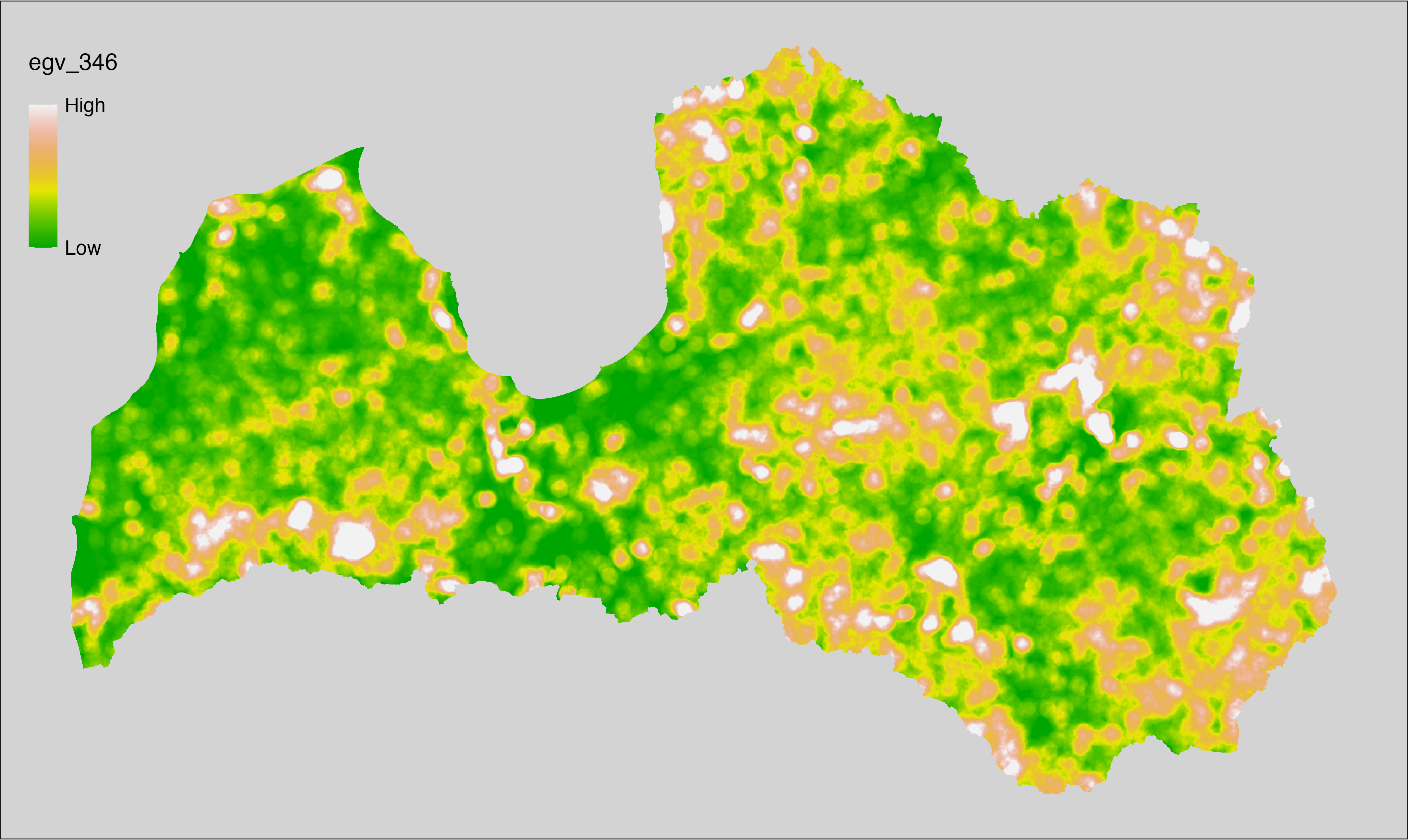
6.347 ForestsTreesAge_BorealDeciduousOld_r10000
filename: ForestsTreesAge_BorealDeciduousOld_r10000.tif
layername: egv_347
English name: Fractional cover of Old (over rotation age) Boreal Deciduous Forests within the 10 km landscape
Latvian name: Vecu (kopš cirtmeta) šaurlapju mežu platības īpatsvars 10 km ainavā
Procedure: The cover fraction within a radius of 10000 m around the analysis grid cell
is calculated as the area-weighted sum of the analysis cells inside
the buffer, using the workflow egvtools::radius_function(). During the calculation of the landscape
metric, inverse distance weighted (power = 2) gap filling on the output is
applied to ensure no missing values at the edges. Then the layer is
rewritten to set its name. Finally, the layer is standardised by
subtracting the arithmetic mean and dividing by the root mean squared error.
Code
# libs ----
if(!require(terra)) {install.packages("terra"); require(terra)}
if(!require(egvtools)) {remotes::install_github("aavotins/egvtools"); require(egvtools)}
# Templates -----
template100=rast("./Templates/TemplateRasters/LV100m_10km.tif")
# radii ----
radius_function(
kvadrati_path = "./Templates/TemplateGrids/tiles/",
radii_path = "./Templates/TemplateGridPoints/tiles/",
tikls100_path = "./Templates/TemplateGrids/tikls100_sauzeme.parquet",
template_path = "./Templates/TemplateRasters/LV100m_10km.tif",
input_layers = c("./RasterGrids_100m/2024/RAW/ForestsTreesAge_BorealDeciduousOld_cell.tif"),
layer_prefixes = c("ForestsTreesAge_BorealDeciduousOld"),
output_dir = "./RasterGrids_100m/2024/RAW/",
n_workers = 6,
radii = c("r10000"),
radius_mode = "sparse",
extract_fun = "mean",
fill_missing = TRUE,
IDW_weight = 2,
future_max_size = 40 * 1024^3)
# ForestsTreesAge_BorealDeciduousOld_r10000.tif egv_347
slanis=rast("./RasterGrids_100m/2024/RAW/ForestsTreesAge_BorealDeciduousOld_r10000.tif")
names(slanis)="egv_347"
slanis2=project(slanis,template100)
writeRaster(slanis2,
"./RasterGrids_100m/2024/RAW/ForestsTreesAge_BorealDeciduousOld_r10000.tif",
overwrite=TRUE)
# standardisation ----
if(!require(terra)) {install.packages("terra"); require(terra)}
if(!require(tidyverse)) {install.packages("tidyverse"); require(tidyverse)}
nosaukums="ForestsTreesAge_BorealDeciduousOld_r10000.tif"
ielasisanas_cels=paste0("./RasterGrids_100m/2024/RAW/",nosaukums)
saglabasanas_cels=paste0("./RasterGrids_100m/2024/Scaled/",nosaukums)
slanis=rast(ielasisanas_cels)
videjais=global(slanis,fun="mean",na.rm=TRUE)
centrets=slanis-videjais[,1]
standartnovirze=terra::global(centrets,fun="rms",na.rm=TRUE)
merogots=centrets/standartnovirze[,1]
writeRaster(merogots,
filename=saglabasanas_cels,
overwrite=TRUE)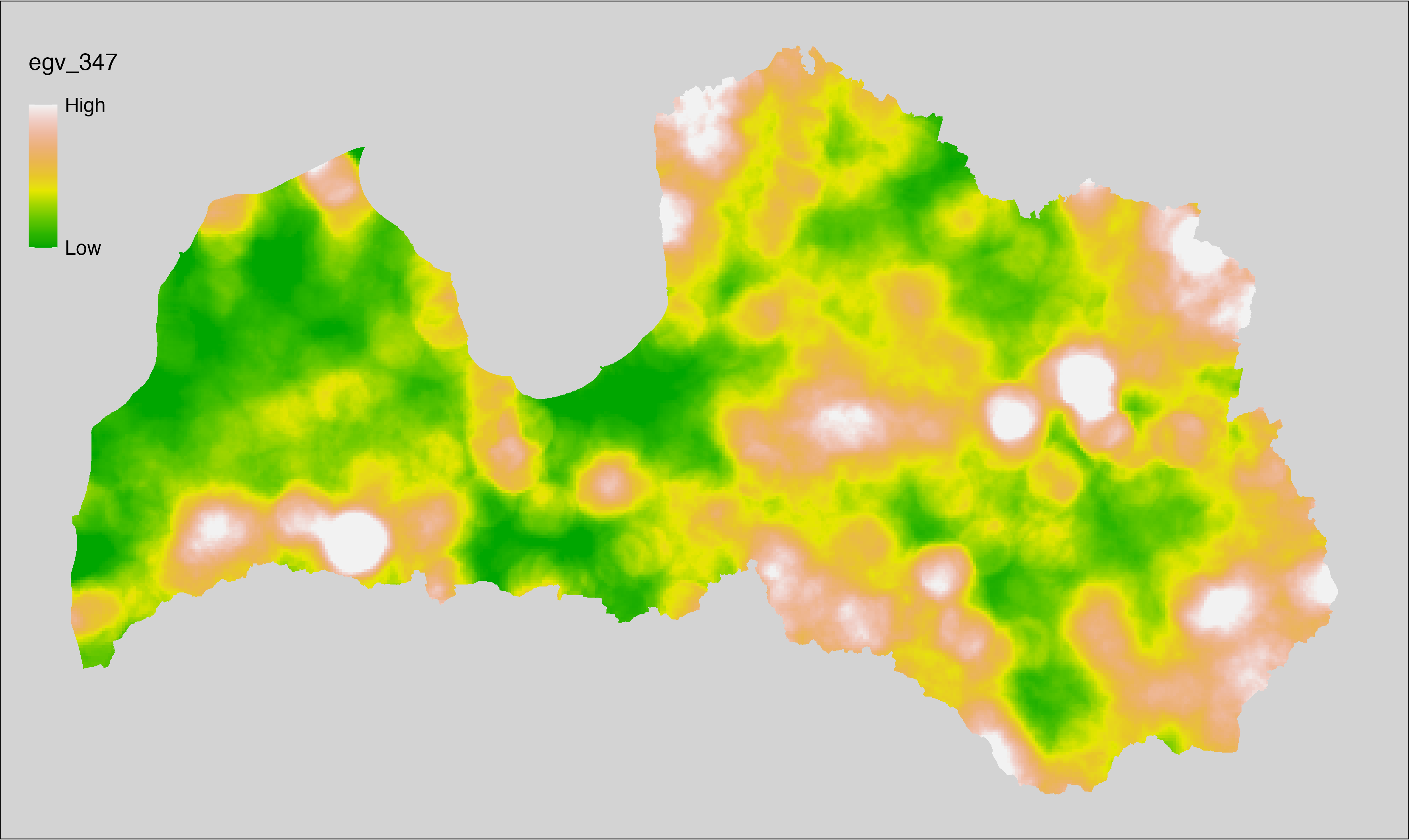
6.348 ForestsTreesAge_BorealDeciduousYoung_cell
filename: ForestsTreesAge_BorealDeciduousYoung_cell.tif
layername: egv_348
English name: Fractional cover of Young (pre-rotation age) Boreal Deciduous Forests within the analysis cell (1 ha)
Latvian name: Jaunu (pirms cirtmeta) šaurlapju mežu platības īpatsvars analīzes šūnā (1 ha)
Procedure: Most EGVs describing forests are spatially restricted to areas outside of clearcuts and dead stands. This mask is created using a combination of the State Forest Service’s State Forest Registry land category 12 and 14, and The Global Forest Watch pixels classified as lost tree canopy cover since 2020 (raster layer matching input, presence = 1, absence = 0).
To prepare this EGV, stands from the State Forest Service’s State Forest Registry are classified into (in order):
coniferous (see Terminology and acronyms for species codes) if timber volume of those species exceeded 75%;
Boreal deciduous if timber volume of those species exceeded 75%;
temperate deciduous if timber volume of those species exceeded 50%;
mixed otherwise;
then Boreal deciduous stands younger than the legal rotation age are selected
and geometries are rasterised (presence = 1, NA otherwise). Rasterisation is
performed using the workflow egvtools::polygon2input(), restricting to pixels outside clearcut
mask and covering background with value 0. The resulting layer
is then aggregated to EGV resolution using the workflow egvtools::input2egv(), which
calculates the arithmetic mean to determine the cover fraction. During
aggregation, inverse distance weighted (power = 2) gap filling on the output is
applied to ensure no missing values at the edges. Finally, the layer is
standardised by subtracting the arithmetic mean and dividing by the root mean squared
error.
Code
# libs ----
if(!require(egvtools)) {remotes::install_github("aavotins/egvtools"); require(egvtools)}
if(!require(terra)) {install.packages("terra"); require(terra)}
if(!require(sf)) {install.packages("sf"); require(sf)}
if(!require(tidyverse)) {install.packages("tidyverse"); require(tidyverse)}
if(!require(sfarrow)) {install.packages("sfarrow"); require(sfarrow)}
if(!require(readxl)) {install.packages("readxl"); require(readxl)}
if(!require(raster)) {install.packages("raster"); require(raster)}
if(!require(fasterize)) {install.packages("fasterize"); require(fasterize)}
# templates ----
template100=rast("./Templates/TemplateRasters/LV100m_10km.tif")
template10=rast("./Templates/TemplateRasters/LV10m_10km.tif")
rastrs10=raster(template10)
nulls10=rast("./Templates/TemplateRasters/nulls_LV10m_10km.tif")
nulls100=rast("./Templates/TemplateRasters/nulls_LV100m_10km.tif")
# simple landscape ----
simple_landscape=rast("RasterGrids_10m/2024/Ainava_vienk_mask.tif")
# mvr ----
mvr=st_read_parquet("./Geodata/2024/MVR/nogabali_2024janv.parquet")
mvr$yes=1
# clear cut mask ----
izcirtumi=mvr %>%
filter(zkat %in% c("12","14")) %>%
dplyr::select(yes)
r_izcirtumi_mvr=fasterize(izcirtumi,rastrs10,field="yes")
t_izcirtumi_mvr=rast(r_izcirtumi_mvr)
plot(t_izcirtumi_mvr)
tcl=rast("./Geodata/2024/Trees/GFW/TreeCoverLoss_v1_12.tif")
tcl2=ifel(tcl<20,0,1)
tclX=cover(tcl2,nulls10)
plot(tclX)
clearcut_mask=cover(t_izcirtumi_mvr,tclX,
filename="./RasterGrids_10m/2024/Mask_clearcuts.tif",
overwrite=TRUE)
plot(clearcut_mask)
rm(izcirtumi)
rm(r_izcirtumi_mvr)
rm(t_izcirtumi_mvr)
rm(tcl)
rm(tcl2)
rm(tclX)
# ForestsTreesAge_BorealDeciduousYoung_cell.tif egv_348 ----
skujkoki=c("1","3","13","14","15","22","23","28") # 8
saurlapji=c("4","6","8","9","19","20","21","32","35","68") # 10
platlapji=c("10","11","12","16","17","18","24","25","26","27","28","29","50",
"61","62","63","64","65","66","67","69") # 21
mvr=mvr %>%
mutate(kraja_skujkoku=ifelse(s10 %in% skujkoki,v10,0)+
ifelse(s11 %in% skujkoki,v11,0)+ifelse(s12 %in% skujkoki,v12,0)+
ifelse(s13 %in% skujkoki,v13,0)+ifelse(s14 %in% skujkoki,v14,0),
kraja_saurlapju=ifelse(s10 %in% saurlapji,v10,0)+
ifelse(s11 %in% saurlapji,v11,0)+ifelse(s12 %in% saurlapji,v12,0)+
ifelse(s13 %in% saurlapji,v13,0)+ifelse(s14 %in% saurlapji,v14,0),
kraja_platlapju=ifelse(s10 %in% platlapji,v10,0)+
ifelse(s11 %in% platlapji,v11,0)+ifelse(s12 %in% platlapji,v12,0)+
ifelse(s13 %in% platlapji,v13,0)+ifelse(s14 %in% platlapji,v14,0)) %>%
mutate(kopeja_kraja=kraja_skujkoku+kraja_platlapju+kraja_saurlapju) %>%
mutate(tips=ifelse(kraja_skujkoku/kopeja_kraja>=0.75,"skujkoku",
ifelse(kraja_saurlapju/kopeja_kraja>=0.75,"saurlapju",
ifelse(kraja_platlapju/kopeja_kraja>0.5,"platlapju",
"jauktu koku"))))
nogabali=mvr %>%
filter(zkat=="10"&tips=="saurlapju"&(vgr=="1"|vgr=="2"|vgr=="3"))
p2i_rez=egvtools::polygon2input(vector_data = nogabali,
template_path = "./Templates/TemplateRasters/LV10m_10km.tif",
out_path = "./RasterGrids_10m/2024/",
file_name = "ForestsTreesAge_BorealDeciduousYoung_input.tif",
value_field = "yes",
restrict_to = clearcut_mask,
restrict_values = 0,
prepare=FALSE,
background_raster = "./Templates/TemplateRasters/nulls_LV10m_10km.tif",
plot_result = TRUE)
p2i_rez
i2e_rez=egvtools::input2egv(input=paste0("./RasterGrids_10m/2024/",
"ForestsTreesAge_BorealDeciduousYoung_input.tif"),
egv_template= "./Templates/TemplateRasters/LV100m_10km.tif",
summary_function = "average",
missing_job = "FillOutput",
outlocation = "./RasterGrids_100m/2024/RAW/",
outfilename = "ForestsTreesAge_BorealDeciduousYoung_cell.tif",
layername = "egv_348",
idw_weight = 2,
plot_gaps = FALSE,plot_final = TRUE)
i2e_rez
rm(nogabali)
rm(p2i_rez)
rm(i2e_rez)
unlink("./RasterGrids_10m/2024/ForestsTreesAge_BorealDeciduousYoung_input.tif")
# standardisation ----
if(!require(terra)) {install.packages("terra"); require(terra)}
if(!require(tidyverse)) {install.packages("tidyverse"); require(tidyverse)}
nosaukums="ForestsTreesAge_BorealDeciduousYoung_cell.tif"
ielasisanas_cels=paste0("./RasterGrids_100m/2024/RAW/",nosaukums)
saglabasanas_cels=paste0("./RasterGrids_100m/2024/Scaled/",nosaukums)
slanis=rast(ielasisanas_cels)
videjais=global(slanis,fun="mean",na.rm=TRUE)
centrets=slanis-videjais[,1]
standartnovirze=terra::global(centrets,fun="rms",na.rm=TRUE)
merogots=centrets/standartnovirze[,1]
writeRaster(merogots,
filename=saglabasanas_cels,
overwrite=TRUE)
6.349 ForestsTreesAge_BorealDeciduousYoung_r500
filename: ForestsTreesAge_BorealDeciduousYoung_r500.tif
layername: egv_349
English name: Fractional cover of Young (pre-rotation age) Boreal Deciduous Forests within the 0.5 km landscape
Latvian name: Jaunu (pirms cirtmeta) šaurlapju mežu platības īpatsvars 0,5 km ainavā
Procedure: The cover fraction within a radius of 500 m around the analysis grid cell is
calculated as the area-weighted sum of the analysis cells inside the
buffer, using the workflow egvtools::radius_function(). During the calculation of the landscape metric,
inverse distance weighted (power = 2) gap filling on the output is applied
to ensure no missing values at the edges. Then the layer is rewritten to set
its name. Finally, the layer is standardised by subtracting the arithmetic
mean and dividing by the root mean squared error.
Code
# libs ----
if(!require(terra)) {install.packages("terra"); require(terra)}
if(!require(egvtools)) {remotes::install_github("aavotins/egvtools"); require(egvtools)}
# Templates -----
template100=rast("./Templates/TemplateRasters/LV100m_10km.tif")
# radii ----
radius_function(
kvadrati_path = "./Templates/TemplateGrids/tiles/",
radii_path = "./Templates/TemplateGridPoints/tiles/",
tikls100_path = "./Templates/TemplateGrids/tikls100_sauzeme.parquet",
template_path = "./Templates/TemplateRasters/LV100m_10km.tif",
input_layers = c("./RasterGrids_100m/2024/RAW/ForestsTreesAge_BorealDeciduousYoung_cell.tif"),
layer_prefixes = c("ForestsTreesAge_BorealDeciduousYoung"),
output_dir = "./RasterGrids_100m/2024/RAW/",
n_workers = 6,
radii = c("r500"),
radius_mode = "sparse",
extract_fun = "mean",
fill_missing = TRUE,
IDW_weight = 2,
future_max_size = 40 * 1024^3)
# ForestsTreesAge_BorealDeciduousYoung_r500.tif egv_349
slanis=rast("./RasterGrids_100m/2024/RAW/ForestsTreesAge_BorealDeciduousYoung_r500.tif")
names(slanis)="egv_349"
slanis2=project(slanis,template100)
writeRaster(slanis2,
"./RasterGrids_100m/2024/RAW/ForestsTreesAge_BorealDeciduousYoung_r500.tif",
overwrite=TRUE)
# standardisation ----
if(!require(terra)) {install.packages("terra"); require(terra)}
if(!require(tidyverse)) {install.packages("tidyverse"); require(tidyverse)}
nosaukums="ForestsTreesAge_BorealDeciduousYoung_r500.tif"
ielasisanas_cels=paste0("./RasterGrids_100m/2024/RAW/",nosaukums)
saglabasanas_cels=paste0("./RasterGrids_100m/2024/Scaled/",nosaukums)
slanis=rast(ielasisanas_cels)
videjais=global(slanis,fun="mean",na.rm=TRUE)
centrets=slanis-videjais[,1]
standartnovirze=terra::global(centrets,fun="rms",na.rm=TRUE)
merogots=centrets/standartnovirze[,1]
writeRaster(merogots,
filename=saglabasanas_cels,
overwrite=TRUE)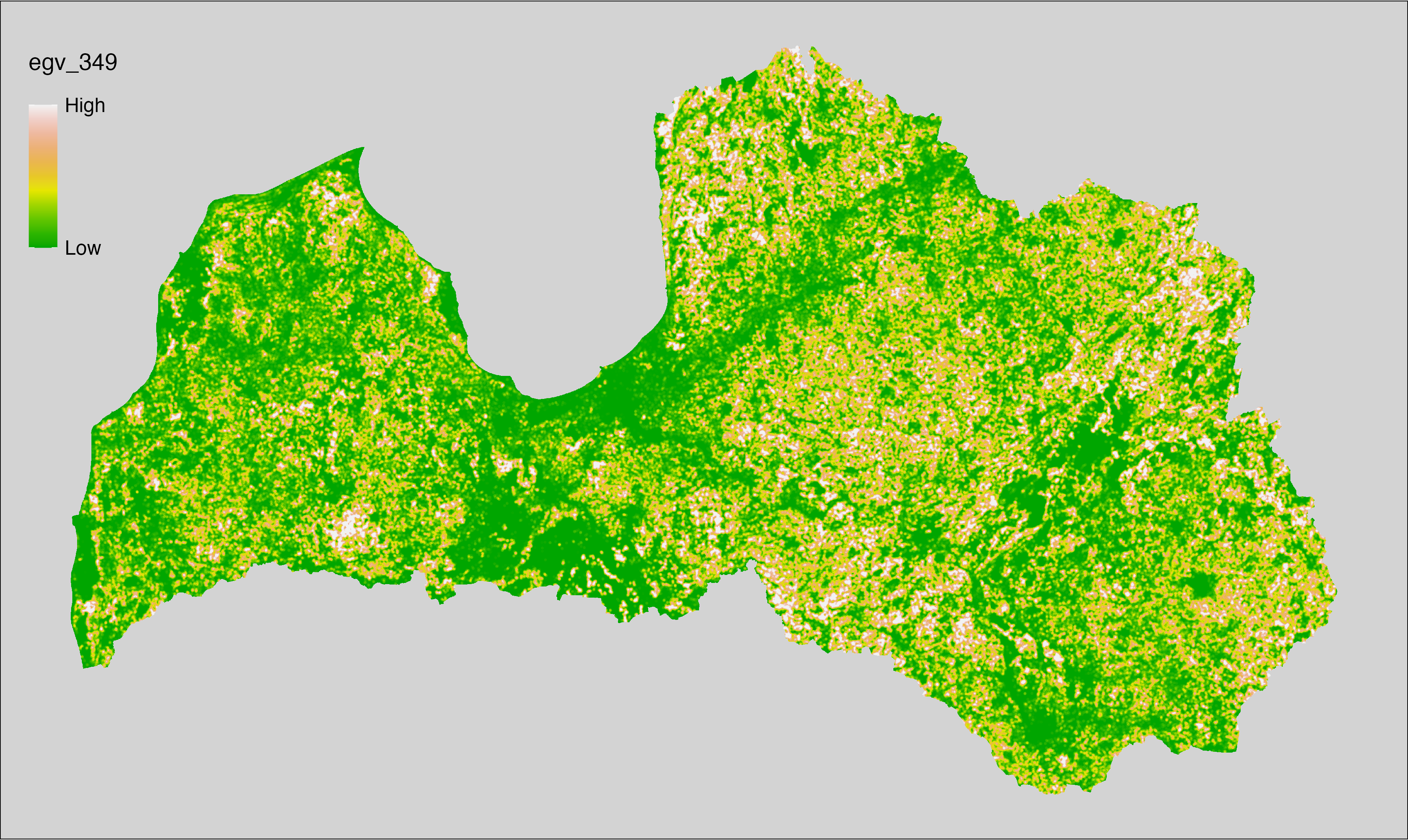
6.350 ForestsTreesAge_BorealDeciduousYoung_r1250
filename: ForestsTreesAge_BorealDeciduousYoung_r1250.tif
layername: egv_350
English name: Fractional cover of Young (pre-rotation age) Boreal Deciduous Forests within the 1.25 km landscape
Latvian name: Jaunu (pirms cirtmeta) šaurlapju mežu platības īpatsvars 1,25 km ainavā
Procedure: The cover fraction within a radius of 1250 m around the analysis grid cell
is calculated as the area-weighted sum of the analysis cells inside
the buffer, using the workflow egvtools::radius_function(). During the calculation of the landscape
metric, inverse distance weighted (power = 2) gap filling on the output is
applied to ensure no missing values at the edges. Then the layer is
rewritten to set its name. Finally, the layer is standardised by
subtracting the arithmetic mean and dividing by the root mean squared error.
Code
# libs ----
if(!require(terra)) {install.packages("terra"); require(terra)}
if(!require(egvtools)) {remotes::install_github("aavotins/egvtools"); require(egvtools)}
# Templates -----
template100=rast("./Templates/TemplateRasters/LV100m_10km.tif")
# radii ----
radius_function(
kvadrati_path = "./Templates/TemplateGrids/tiles/",
radii_path = "./Templates/TemplateGridPoints/tiles/",
tikls100_path = "./Templates/TemplateGrids/tikls100_sauzeme.parquet",
template_path = "./Templates/TemplateRasters/LV100m_10km.tif",
input_layers = c("./RasterGrids_100m/2024/RAW/ForestsTreesAge_BorealDeciduousYoung_cell.tif"),
layer_prefixes = c("ForestsTreesAge_BorealDeciduousYoung"),
output_dir = "./RasterGrids_100m/2024/RAW/",
n_workers = 6,
radii = c("r1250"),
radius_mode = "sparse",
extract_fun = "mean",
fill_missing = TRUE,
IDW_weight = 2,
future_max_size = 40 * 1024^3)
# ForestsTreesAge_BorealDeciduousYoung_r1250.tif egv_350
slanis=rast("./RasterGrids_100m/2024/RAW/ForestsTreesAge_BorealDeciduousYoung_r1250.tif")
names(slanis)="egv_350"
slanis2=project(slanis,template100)
writeRaster(slanis2,
"./RasterGrids_100m/2024/RAW/ForestsTreesAge_BorealDeciduousYoung_r1250.tif",
overwrite=TRUE)
# standardisation ----
if(!require(terra)) {install.packages("terra"); require(terra)}
if(!require(tidyverse)) {install.packages("tidyverse"); require(tidyverse)}
nosaukums="ForestsTreesAge_BorealDeciduousYoung_r1250.tif"
ielasisanas_cels=paste0("./RasterGrids_100m/2024/RAW/",nosaukums)
saglabasanas_cels=paste0("./RasterGrids_100m/2024/Scaled/",nosaukums)
slanis=rast(ielasisanas_cels)
videjais=global(slanis,fun="mean",na.rm=TRUE)
centrets=slanis-videjais[,1]
standartnovirze=terra::global(centrets,fun="rms",na.rm=TRUE)
merogots=centrets/standartnovirze[,1]
writeRaster(merogots,
filename=saglabasanas_cels,
overwrite=TRUE)
6.351 ForestsTreesAge_BorealDeciduousYoung_r3000
filename: ForestsTreesAge_BorealDeciduousYoung_r3000.tif
layername: egv_351
English name: Fractional cover of Young (pre-rotation age) Boreal Deciduous Forests within the 3 km landscape
Latvian name: Jaunu (pirms cirtmeta) šaurlapju mežu platības īpatsvars 3 km ainavā
Procedure: The cover fraction within a radius of 3000 m around the analysis grid cell
is calculated as the area-weighted sum of the analysis cells inside
the buffer, using the workflow egvtools::radius_function(). During the calculation of the landscape
metric, inverse distance weighted (power = 2) gap filling on the output is
applied to ensure no missing values at the edges. Then the layer is
rewritten to set its name. Finally, the layer is standardised by
subtracting the arithmetic mean and dividing by the root mean squared error.
Code
# libs ----
if(!require(terra)) {install.packages("terra"); require(terra)}
if(!require(egvtools)) {remotes::install_github("aavotins/egvtools"); require(egvtools)}
# Templates -----
template100=rast("./Templates/TemplateRasters/LV100m_10km.tif")
# radii ----
radius_function(
kvadrati_path = "./Templates/TemplateGrids/tiles/",
radii_path = "./Templates/TemplateGridPoints/tiles/",
tikls100_path = "./Templates/TemplateGrids/tikls100_sauzeme.parquet",
template_path = "./Templates/TemplateRasters/LV100m_10km.tif",
input_layers = c("./RasterGrids_100m/2024/RAW/ForestsTreesAge_BorealDeciduousYoung_cell.tif"),
layer_prefixes = c("ForestsTreesAge_BorealDeciduousYoung"),
output_dir = "./RasterGrids_100m/2024/RAW/",
n_workers = 6,
radii = c("r3000"),
radius_mode = "sparse",
extract_fun = "mean",
fill_missing = TRUE,
IDW_weight = 2,
future_max_size = 40 * 1024^3)
# ForestsTreesAge_BorealDeciduousYoung_r3000.tif egv_351
slanis=rast("./RasterGrids_100m/2024/RAW/ForestsTreesAge_BorealDeciduousYoung_r3000.tif")
names(slanis)="egv_351"
slanis2=project(slanis,template100)
writeRaster(slanis2,
"./RasterGrids_100m/2024/RAW/ForestsTreesAge_BorealDeciduousYoung_r3000.tif",
overwrite=TRUE)
# standardisation ----
if(!require(terra)) {install.packages("terra"); require(terra)}
if(!require(tidyverse)) {install.packages("tidyverse"); require(tidyverse)}
nosaukums="ForestsTreesAge_BorealDeciduousYoung_r3000.tif"
ielasisanas_cels=paste0("./RasterGrids_100m/2024/RAW/",nosaukums)
saglabasanas_cels=paste0("./RasterGrids_100m/2024/Scaled/",nosaukums)
slanis=rast(ielasisanas_cels)
videjais=global(slanis,fun="mean",na.rm=TRUE)
centrets=slanis-videjais[,1]
standartnovirze=terra::global(centrets,fun="rms",na.rm=TRUE)
merogots=centrets/standartnovirze[,1]
writeRaster(merogots,
filename=saglabasanas_cels,
overwrite=TRUE)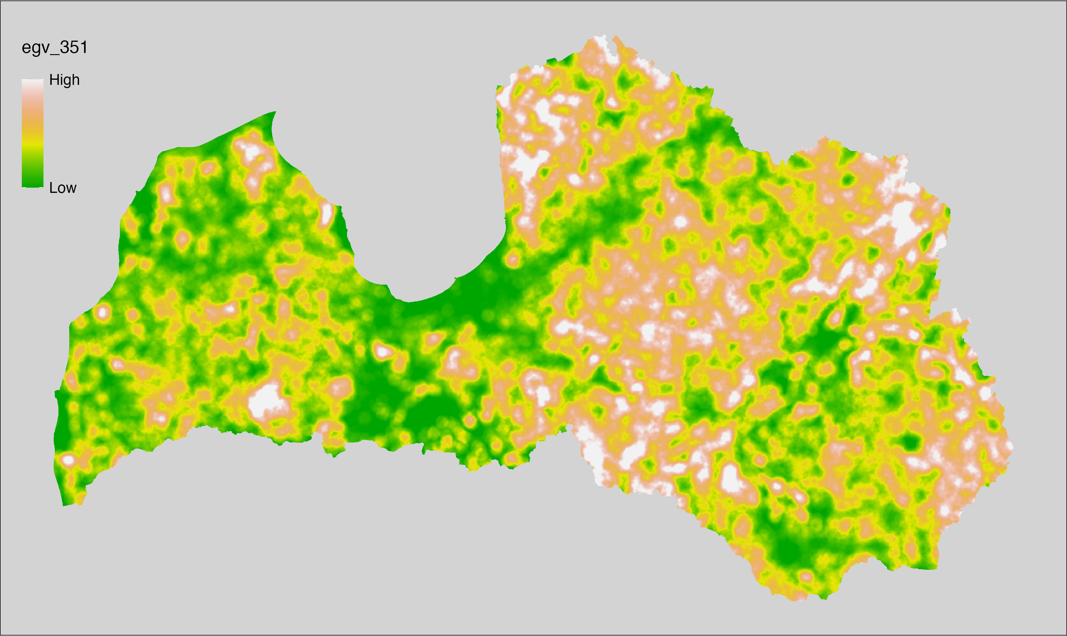
6.352 ForestsTreesAge_BorealDeciduousYoung_r10000
filename: ForestsTreesAge_BorealDeciduousYoung_r10000.tif
layername: egv_352
English name: Fractional cover of Young (pre-rotation age) Boreal Deciduous Forests within the 10 km landscape
Latvian name: Jaunu (pirms cirtmeta) šaurlapju mežu platības īpatsvars 10 km ainavā
Procedure: The cover fraction within a radius of 10000 m around the analysis grid cell
is calculated as the area-weighted sum of the analysis cells inside
the buffer, using the workflow egvtools::radius_function(). During the calculation of the landscape
metric, inverse distance weighted (power = 2) gap filling on the output is
applied to ensure no missing values at the edges. Then the layer is
rewritten to set its name. Finally, the layer is standardised by
subtracting the arithmetic mean and dividing by the root mean squared error.
Code
# libs ----
if(!require(terra)) {install.packages("terra"); require(terra)}
if(!require(egvtools)) {remotes::install_github("aavotins/egvtools"); require(egvtools)}
# Templates -----
template100=rast("./Templates/TemplateRasters/LV100m_10km.tif")
# radii ----
radius_function(
kvadrati_path = "./Templates/TemplateGrids/tiles/",
radii_path = "./Templates/TemplateGridPoints/tiles/",
tikls100_path = "./Templates/TemplateGrids/tikls100_sauzeme.parquet",
template_path = "./Templates/TemplateRasters/LV100m_10km.tif",
input_layers = c("./RasterGrids_100m/2024/RAW/ForestsTreesAge_BorealDeciduousYoung_cell.tif"),
layer_prefixes = c("ForestsTreesAge_BorealDeciduousYoung"),
output_dir = "./RasterGrids_100m/2024/RAW/",
n_workers = 6,
radii = c("r10000"),
radius_mode = "sparse",
extract_fun = "mean",
fill_missing = TRUE,
IDW_weight = 2,
future_max_size = 40 * 1024^3)
# ForestsTreesAge_BorealDeciduousYoung_r10000.tif egv_352
slanis=rast("./RasterGrids_100m/2024/RAW/ForestsTreesAge_BorealDeciduousYoung_r10000.tif")
names(slanis)="egv_352"
slanis2=project(slanis,template100)
writeRaster(slanis2,
"./RasterGrids_100m/2024/RAW/ForestsTreesAge_BorealDeciduousYoung_r10000.tif",
overwrite=TRUE)
# standardisation ----
if(!require(terra)) {install.packages("terra"); require(terra)}
if(!require(tidyverse)) {install.packages("tidyverse"); require(tidyverse)}
nosaukums="ForestsTreesAge_BorealDeciduousYoung_r10000.tif"
ielasisanas_cels=paste0("./RasterGrids_100m/2024/RAW/",nosaukums)
saglabasanas_cels=paste0("./RasterGrids_100m/2024/Scaled/",nosaukums)
slanis=rast(ielasisanas_cels)
videjais=global(slanis,fun="mean",na.rm=TRUE)
centrets=slanis-videjais[,1]
standartnovirze=terra::global(centrets,fun="rms",na.rm=TRUE)
merogots=centrets/standartnovirze[,1]
writeRaster(merogots,
filename=saglabasanas_cels,
overwrite=TRUE)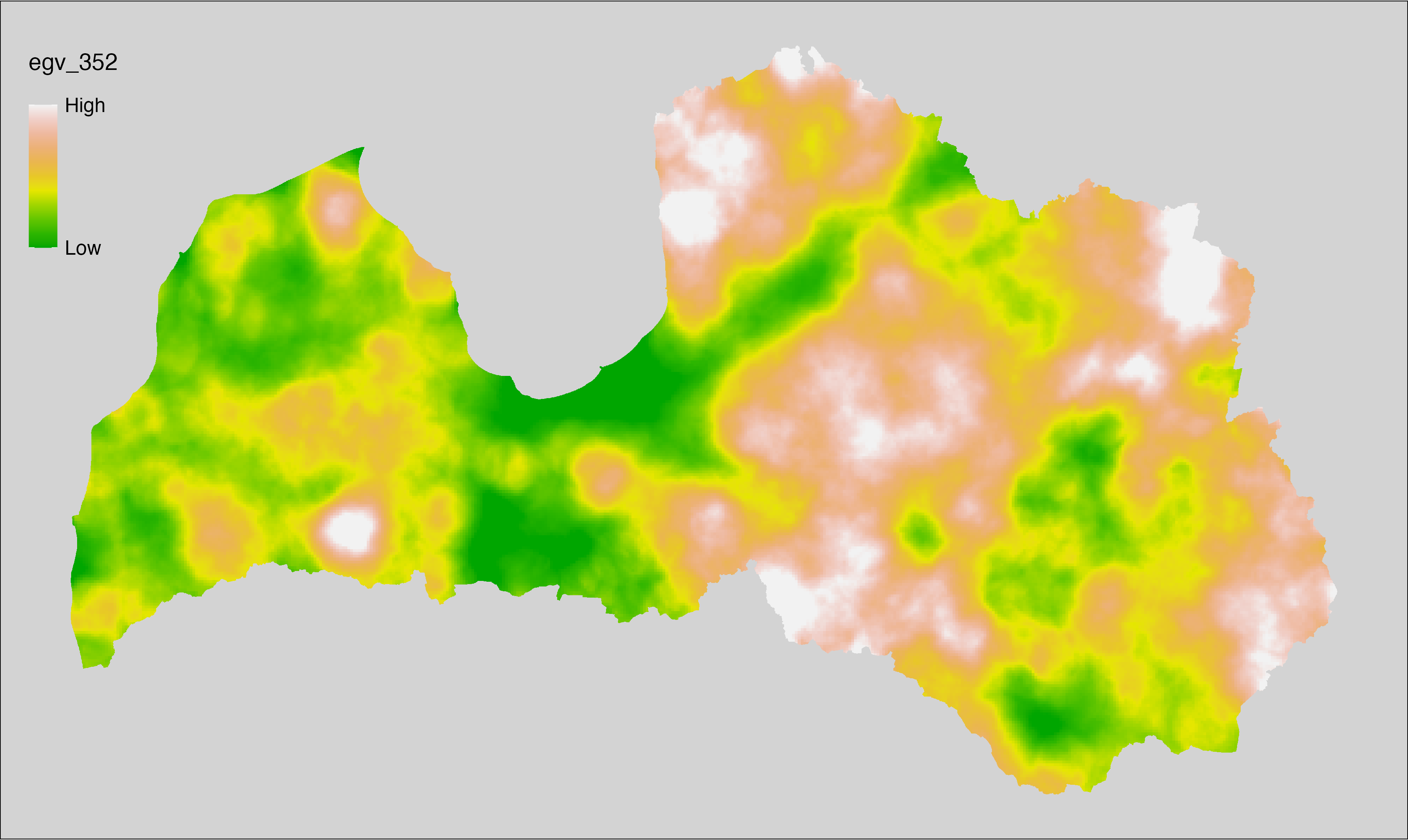
6.353 ForestsTreesAge_ConiferousOld_cell
filename: ForestsTreesAge_ConiferousOld_cell.tif
layername: egv_353
English name: Fractional cover of Old (over rotation age) Coniferous Forests within the analysis cell (1 ha)
Latvian name: Vecu (kopš cirtmeta) skujkoku mežu platības īpatsvars analīzes šūnā (1 ha)
Procedure: Most EGVs describing forests are spatially restricted to areas outside of clearcuts and dead stands. This mask is created using a combination of the State Forest Service’s State Forest Registry land category 12 and 14, and The Global Forest Watch pixels classified as lost tree canopy cover since 2020 (raster layer matching input, presence = 1, absence = 0).
To prepare this EGV, stands from the State Forest Service’s State Forest Registry are classified into (in order):
coniferous (see Terminology and acronyms for species codes) if timber volume of those species exceeded 75%;
Boreal deciduous if timber volume of those species exceeded 75%;
temperate deciduous if timber volume of those species exceeded 50%;
mixed otherwise;
then coniferous stands exceeding the legal rotation age are selected and
geometries are rasterised (presence = 1, NA otherwise). Rasterisation is
performed using the workflow egvtools::polygon2input(), restricting to pixels outside clearcut
mask and covering background with value 0. The resulting layer
is then aggregated to EGV resolution using the workflow egvtools::input2egv(), which
calculates the arithmetic mean to determine the cover fraction. During
aggregation, inverse distance weighted (power = 2) gap filling on the output is
applied to ensure no missing values at the edges. Finally, the layer is
standardised by subtracting the arithmetic mean and dividing by the root mean squared
error.
Code
# libs ----
if(!require(egvtools)) {remotes::install_github("aavotins/egvtools"); require(egvtools)}
if(!require(terra)) {install.packages("terra"); require(terra)}
if(!require(sf)) {install.packages("sf"); require(sf)}
if(!require(tidyverse)) {install.packages("tidyverse"); require(tidyverse)}
if(!require(sfarrow)) {install.packages("sfarrow"); require(sfarrow)}
if(!require(readxl)) {install.packages("readxl"); require(readxl)}
if(!require(raster)) {install.packages("raster"); require(raster)}
if(!require(fasterize)) {install.packages("fasterize"); require(fasterize)}
# templates ----
template100=rast("./Templates/TemplateRasters/LV100m_10km.tif")
template10=rast("./Templates/TemplateRasters/LV10m_10km.tif")
rastrs10=raster(template10)
nulls10=rast("./Templates/TemplateRasters/nulls_LV10m_10km.tif")
nulls100=rast("./Templates/TemplateRasters/nulls_LV100m_10km.tif")
# simple landscape ----
simple_landscape=rast("RasterGrids_10m/2024/Ainava_vienk_mask.tif")
# mvr ----
mvr=st_read_parquet("./Geodata/2024/MVR/nogabali_2024janv.parquet")
mvr$yes=1
# clear cut mask ----
izcirtumi=mvr %>%
filter(zkat %in% c("12","14")) %>%
dplyr::select(yes)
r_izcirtumi_mvr=fasterize(izcirtumi,rastrs10,field="yes")
t_izcirtumi_mvr=rast(r_izcirtumi_mvr)
plot(t_izcirtumi_mvr)
tcl=rast("./Geodata/2024/Trees/GFW/TreeCoverLoss_v1_12.tif")
tcl2=ifel(tcl<20,0,1)
tclX=cover(tcl2,nulls10)
plot(tclX)
clearcut_mask=cover(t_izcirtumi_mvr,tclX,
filename="./RasterGrids_10m/2024/Mask_clearcuts.tif",
overwrite=TRUE)
plot(clearcut_mask)
rm(izcirtumi)
rm(r_izcirtumi_mvr)
rm(t_izcirtumi_mvr)
rm(tcl)
rm(tcl2)
rm(tclX)
# ForestsTreesAge_ConiferousOld_cell.tif egv_353 ----
skujkoki=c("1","3","13","14","15","22","23","28") # 8
saurlapji=c("4","6","8","9","19","20","21","32","35","68") # 10
platlapji=c("10","11","12","16","17","18","24","25","26","27","28","29","50",
"61","62","63","64","65","66","67","69") # 21
mvr=mvr %>%
mutate(kraja_skujkoku=ifelse(s10 %in% skujkoki,v10,0)+
ifelse(s11 %in% skujkoki,v11,0)+ifelse(s12 %in% skujkoki,v12,0)+
ifelse(s13 %in% skujkoki,v13,0)+ifelse(s14 %in% skujkoki,v14,0),
kraja_saurlapju=ifelse(s10 %in% saurlapji,v10,0)+
ifelse(s11 %in% saurlapji,v11,0)+ifelse(s12 %in% saurlapji,v12,0)+
ifelse(s13 %in% saurlapji,v13,0)+ifelse(s14 %in% saurlapji,v14,0),
kraja_platlapju=ifelse(s10 %in% platlapji,v10,0)+
ifelse(s11 %in% platlapji,v11,0)+ifelse(s12 %in% platlapji,v12,0)+
ifelse(s13 %in% platlapji,v13,0)+ifelse(s14 %in% platlapji,v14,0)) %>%
mutate(kopeja_kraja=kraja_skujkoku+kraja_platlapju+kraja_saurlapju) %>%
mutate(tips=ifelse(kraja_skujkoku/kopeja_kraja>=0.75,"skujkoku",
ifelse(kraja_saurlapju/kopeja_kraja>=0.75,"saurlapju",
ifelse(kraja_platlapju/kopeja_kraja>0.5,"platlapju",
"jauktu koku"))))
nogabali=mvr %>%
filter(zkat=="10"&tips=="skujkoku"&(vgr=="4"|vgr=="5"))
p2i_rez=egvtools::polygon2input(vector_data = nogabali,
template_path = "./Templates/TemplateRasters/LV10m_10km.tif",
out_path = "./RasterGrids_10m/2024/",
file_name = "ForestsTreesAge_ConiferousOld_input.tif",
value_field = "yes",
restrict_to = clearcut_mask,
restrict_values = 0,
prepare=FALSE,
background_raster = "./Templates/TemplateRasters/nulls_LV10m_10km.tif",
plot_result = TRUE)
p2i_rez
i2e_rez=egvtools::input2egv(input=paste0("./RasterGrids_10m/2024/",
"ForestsTreesAge_ConiferousOld_input.tif"),
egv_template= "./Templates/TemplateRasters/LV100m_10km.tif",
summary_function = "average",
missing_job = "FillOutput",
outlocation = "./RasterGrids_100m/2024/RAW/",
outfilename = "ForestsTreesAge_ConiferousOld_cell.tif",
layername = "egv_353",
idw_weight = 2,
plot_gaps = FALSE,plot_final = TRUE)
i2e_rez
rm(nogabali)
rm(p2i_rez)
rm(i2e_rez)
unlink("./RasterGrids_10m/2024/ForestsTreesAge_ConiferousOld_input.tif")
# standardisation ----
if(!require(terra)) {install.packages("terra"); require(terra)}
if(!require(tidyverse)) {install.packages("tidyverse"); require(tidyverse)}
nosaukums="ForestsTreesAge_ConiferousOld_cell.tif"
ielasisanas_cels=paste0("./RasterGrids_100m/2024/RAW/",nosaukums)
saglabasanas_cels=paste0("./RasterGrids_100m/2024/Scaled/",nosaukums)
slanis=rast(ielasisanas_cels)
videjais=global(slanis,fun="mean",na.rm=TRUE)
centrets=slanis-videjais[,1]
standartnovirze=terra::global(centrets,fun="rms",na.rm=TRUE)
merogots=centrets/standartnovirze[,1]
writeRaster(merogots,
filename=saglabasanas_cels,
overwrite=TRUE)
6.354 ForestsTreesAge_ConiferousOld_r500
filename: ForestsTreesAge_ConiferousOld_r500.tif
layername: egv_354
English name: Fractional cover of Old (over rotation age) Coniferous Forests within the 0.5 km landscape
Latvian name: Vecu (kopš cirtmeta) skujkoku mežu platības īpatsvars 0,5 km ainavā
Procedure: The cover fraction within a radius of 500 m around the analysis grid cell is
calculated as the area-weighted sum of the analysis cells inside the
buffer, using the workflow egvtools::radius_function(). During the calculation of the landscape metric,
inverse distance weighted (power = 2) gap filling on the output is applied
to ensure no missing values at the edges. Then the layer is rewritten to set
its name. Finally, the layer is standardised by subtracting the arithmetic
mean and dividing by the root mean squared error.
Code
# libs ----
if(!require(terra)) {install.packages("terra"); require(terra)}
if(!require(egvtools)) {remotes::install_github("aavotins/egvtools"); require(egvtools)}
# Templates -----
template100=rast("./Templates/TemplateRasters/LV100m_10km.tif")
# radii ----
radius_function(
kvadrati_path = "./Templates/TemplateGrids/tiles/",
radii_path = "./Templates/TemplateGridPoints/tiles/",
tikls100_path = "./Templates/TemplateGrids/tikls100_sauzeme.parquet",
template_path = "./Templates/TemplateRasters/LV100m_10km.tif",
input_layers = c("./RasterGrids_100m/2024/RAW/ForestsTreesAge_ConiferousOld_cell.tif"),
layer_prefixes = c("ForestsTreesAge_ConiferousOld"),
output_dir = "./RasterGrids_100m/2024/RAW/",
n_workers = 6,
radii = c("r500"),
radius_mode = "sparse",
extract_fun = "mean",
fill_missing = TRUE,
IDW_weight = 2,
future_max_size = 40 * 1024^3)
# ForestsTreesAge_ConiferousOld_r500.tif egv_354
slanis=rast("./RasterGrids_100m/2024/RAW/ForestsTreesAge_ConiferousOld_r500.tif")
names(slanis)="egv_354"
slanis2=project(slanis,template100)
writeRaster(slanis2,
"./RasterGrids_100m/2024/RAW/ForestsTreesAge_ConiferousOld_r500.tif",
overwrite=TRUE)
# standardisation ----
if(!require(terra)) {install.packages("terra"); require(terra)}
if(!require(tidyverse)) {install.packages("tidyverse"); require(tidyverse)}
nosaukums="ForestsTreesAge_ConiferousOld_r500.tif"
ielasisanas_cels=paste0("./RasterGrids_100m/2024/RAW/",nosaukums)
saglabasanas_cels=paste0("./RasterGrids_100m/2024/Scaled/",nosaukums)
slanis=rast(ielasisanas_cels)
videjais=global(slanis,fun="mean",na.rm=TRUE)
centrets=slanis-videjais[,1]
standartnovirze=terra::global(centrets,fun="rms",na.rm=TRUE)
merogots=centrets/standartnovirze[,1]
writeRaster(merogots,
filename=saglabasanas_cels,
overwrite=TRUE)
6.355 ForestsTreesAge_ConiferousOld_r1250
filename: ForestsTreesAge_ConiferousOld_r1250.tif
layername: egv_355
English name: Fractional cover of Old (over rotation age) Coniferous Forests within the 1.25 km landscape
Latvian name: Vecu (kopš cirtmeta) skujkoku mežu platības īpatsvars 1,25 km ainavā
Procedure: The cover fraction within a radius of 1250 m around the analysis grid cell
is calculated as the area-weighted sum of the analysis cells inside
the buffer, using the workflow egvtools::radius_function(). During the calculation of the landscape
metric, inverse distance weighted (power = 2) gap filling on the output is
applied to ensure no missing values at the edges. Then the layer is
rewritten to set its name. Finally, the layer is standardised by
subtracting the arithmetic mean and dividing by the root mean squared error.
Code
# libs ----
if(!require(terra)) {install.packages("terra"); require(terra)}
if(!require(egvtools)) {remotes::install_github("aavotins/egvtools"); require(egvtools)}
# Templates -----
template100=rast("./Templates/TemplateRasters/LV100m_10km.tif")
# radii ----
radius_function(
kvadrati_path = "./Templates/TemplateGrids/tiles/",
radii_path = "./Templates/TemplateGridPoints/tiles/",
tikls100_path = "./Templates/TemplateGrids/tikls100_sauzeme.parquet",
template_path = "./Templates/TemplateRasters/LV100m_10km.tif",
input_layers = c("./RasterGrids_100m/2024/RAW/ForestsTreesAge_ConiferousOld_cell.tif"),
layer_prefixes = c("ForestsTreesAge_ConiferousOld"),
output_dir = "./RasterGrids_100m/2024/RAW/",
n_workers = 6,
radii = c("r1250"),
radius_mode = "sparse",
extract_fun = "mean",
fill_missing = TRUE,
IDW_weight = 2,
future_max_size = 40 * 1024^3)
# ForestsTreesAge_ConiferousOld_r1250.tif egv_355
slanis=rast("./RasterGrids_100m/2024/RAW/ForestsTreesAge_ConiferousOld_r1250.tif")
names(slanis)="egv_355"
slanis2=project(slanis,template100)
writeRaster(slanis2,
"./RasterGrids_100m/2024/RAW/ForestsTreesAge_ConiferousOld_r1250.tif",
overwrite=TRUE)
# standardisation ----
if(!require(terra)) {install.packages("terra"); require(terra)}
if(!require(tidyverse)) {install.packages("tidyverse"); require(tidyverse)}
nosaukums="ForestsTreesAge_ConiferousOld_r1250.tif"
ielasisanas_cels=paste0("./RasterGrids_100m/2024/RAW/",nosaukums)
saglabasanas_cels=paste0("./RasterGrids_100m/2024/Scaled/",nosaukums)
slanis=rast(ielasisanas_cels)
videjais=global(slanis,fun="mean",na.rm=TRUE)
centrets=slanis-videjais[,1]
standartnovirze=terra::global(centrets,fun="rms",na.rm=TRUE)
merogots=centrets/standartnovirze[,1]
writeRaster(merogots,
filename=saglabasanas_cels,
overwrite=TRUE)
6.356 ForestsTreesAge_ConiferousOld_r3000
filename: ForestsTreesAge_ConiferousOld_r3000.tif
layername: egv_356
English name: Fractional cover of Old (over rotation age) Coniferous Forests within the 3 km landscape
Latvian name: Vecu (kopš cirtmeta) skujkoku mežu platības īpatsvars 3 km ainavā
Procedure: The cover fraction within a radius of 3000 m around the analysis grid cell
is calculated as the area-weighted sum of the analysis cells inside
the buffer, using the workflow egvtools::radius_function(). During the calculation of the landscape
metric, inverse distance weighted (power = 2) gap filling on the output is
applied to ensure no missing values at the edges. Then the layer is
rewritten to set its name. Finally, the layer is standardised by
subtracting the arithmetic mean and dividing by the root mean squared error.
Code
# libs ----
if(!require(terra)) {install.packages("terra"); require(terra)}
if(!require(egvtools)) {remotes::install_github("aavotins/egvtools"); require(egvtools)}
# Templates -----
template100=rast("./Templates/TemplateRasters/LV100m_10km.tif")
# radii ----
radius_function(
kvadrati_path = "./Templates/TemplateGrids/tiles/",
radii_path = "./Templates/TemplateGridPoints/tiles/",
tikls100_path = "./Templates/TemplateGrids/tikls100_sauzeme.parquet",
template_path = "./Templates/TemplateRasters/LV100m_10km.tif",
input_layers = c("./RasterGrids_100m/2024/RAW/ForestsTreesAge_ConiferousOld_cell.tif"),
layer_prefixes = c("ForestsTreesAge_ConiferousOld"),
output_dir = "./RasterGrids_100m/2024/RAW/",
n_workers = 6,
radii = c("r3000"),
radius_mode = "sparse",
extract_fun = "mean",
fill_missing = TRUE,
IDW_weight = 2,
future_max_size = 40 * 1024^3)
# ForestsTreesAge_ConiferousOld_r3000.tif egv_356
slanis=rast("./RasterGrids_100m/2024/RAW/ForestsTreesAge_ConiferousOld_r3000.tif")
names(slanis)="egv_356"
slanis2=project(slanis,template100)
writeRaster(slanis2,
"./RasterGrids_100m/2024/RAW/ForestsTreesAge_ConiferousOld_r3000.tif",
overwrite=TRUE)
# standardisation ----
if(!require(terra)) {install.packages("terra"); require(terra)}
if(!require(tidyverse)) {install.packages("tidyverse"); require(tidyverse)}
nosaukums="ForestsTreesAge_ConiferousOld_r3000.tif"
ielasisanas_cels=paste0("./RasterGrids_100m/2024/RAW/",nosaukums)
saglabasanas_cels=paste0("./RasterGrids_100m/2024/Scaled/",nosaukums)
slanis=rast(ielasisanas_cels)
videjais=global(slanis,fun="mean",na.rm=TRUE)
centrets=slanis-videjais[,1]
standartnovirze=terra::global(centrets,fun="rms",na.rm=TRUE)
merogots=centrets/standartnovirze[,1]
writeRaster(merogots,
filename=saglabasanas_cels,
overwrite=TRUE)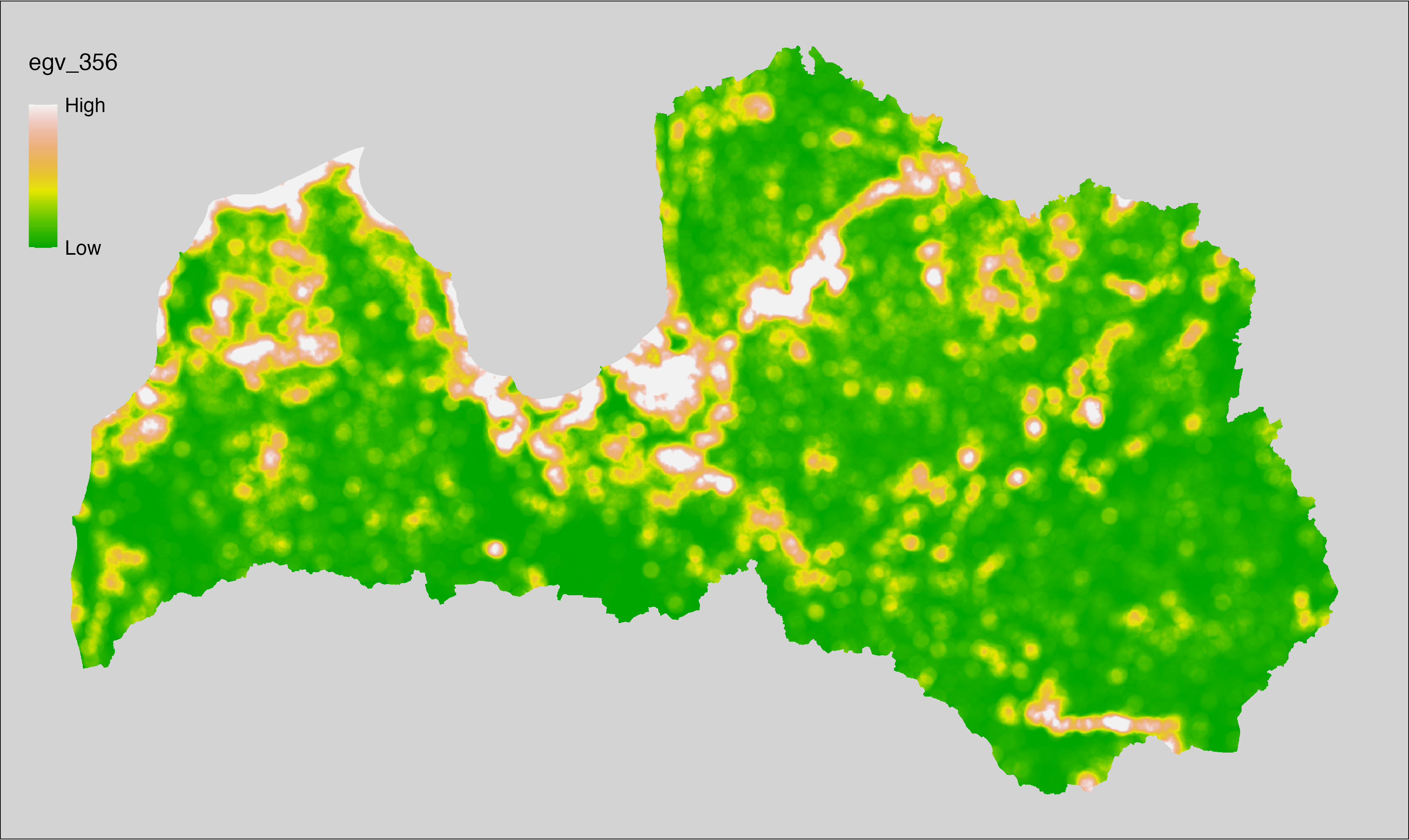
6.357 ForestsTreesAge_ConiferousOld_r10000
filename: ForestsTreesAge_ConiferousOld_r10000.tif
layername: egv_357
English name: Fractional cover of Old (over rotation age) Coniferous Forests within the 10 km landscape
Latvian name: Vecu (kopš cirtmeta) skujkoku mežu platības īpatsvars 10 km ainavā
Procedure: The cover fraction within a radius of 10000 m around the analysis grid cell
is calculated as the area-weighted sum of the analysis cells inside
the buffer, using the workflow egvtools::radius_function(). During the calculation of the landscape
metric, inverse distance weighted (power = 2) gap filling on the output is
applied to ensure no missing values at the edges. Then the layer is
rewritten to set its name. Finally, the layer is standardised by
subtracting the arithmetic mean and dividing by the root mean squared error.
Code
# libs ----
if(!require(terra)) {install.packages("terra"); require(terra)}
if(!require(egvtools)) {remotes::install_github("aavotins/egvtools"); require(egvtools)}
# Templates -----
template100=rast("./Templates/TemplateRasters/LV100m_10km.tif")
# radii ----
radius_function(
kvadrati_path = "./Templates/TemplateGrids/tiles/",
radii_path = "./Templates/TemplateGridPoints/tiles/",
tikls100_path = "./Templates/TemplateGrids/tikls100_sauzeme.parquet",
template_path = "./Templates/TemplateRasters/LV100m_10km.tif",
input_layers = c("./RasterGrids_100m/2024/RAW/ForestsTreesAge_ConiferousOld_cell.tif"),
layer_prefixes = c("ForestsTreesAge_ConiferousOld"),
output_dir = "./RasterGrids_100m/2024/RAW/",
n_workers = 6,
radii = c("r10000"),
radius_mode = "sparse",
extract_fun = "mean",
fill_missing = TRUE,
IDW_weight = 2,
future_max_size = 40 * 1024^3)
# ForestsTreesAge_ConiferousOld_r10000.tif egv_357
slanis=rast("./RasterGrids_100m/2024/RAW/ForestsTreesAge_ConiferousOld_r10000.tif")
names(slanis)="egv_357"
slanis2=project(slanis,template100)
writeRaster(slanis2,
"./RasterGrids_100m/2024/RAW/ForestsTreesAge_ConiferousOld_r10000.tif",
overwrite=TRUE)
# standardisation ----
if(!require(terra)) {install.packages("terra"); require(terra)}
if(!require(tidyverse)) {install.packages("tidyverse"); require(tidyverse)}
nosaukums="ForestsTreesAge_ConiferousOld_r10000.tif"
ielasisanas_cels=paste0("./RasterGrids_100m/2024/RAW/",nosaukums)
saglabasanas_cels=paste0("./RasterGrids_100m/2024/Scaled/",nosaukums)
slanis=rast(ielasisanas_cels)
videjais=global(slanis,fun="mean",na.rm=TRUE)
centrets=slanis-videjais[,1]
standartnovirze=terra::global(centrets,fun="rms",na.rm=TRUE)
merogots=centrets/standartnovirze[,1]
writeRaster(merogots,
filename=saglabasanas_cels,
overwrite=TRUE)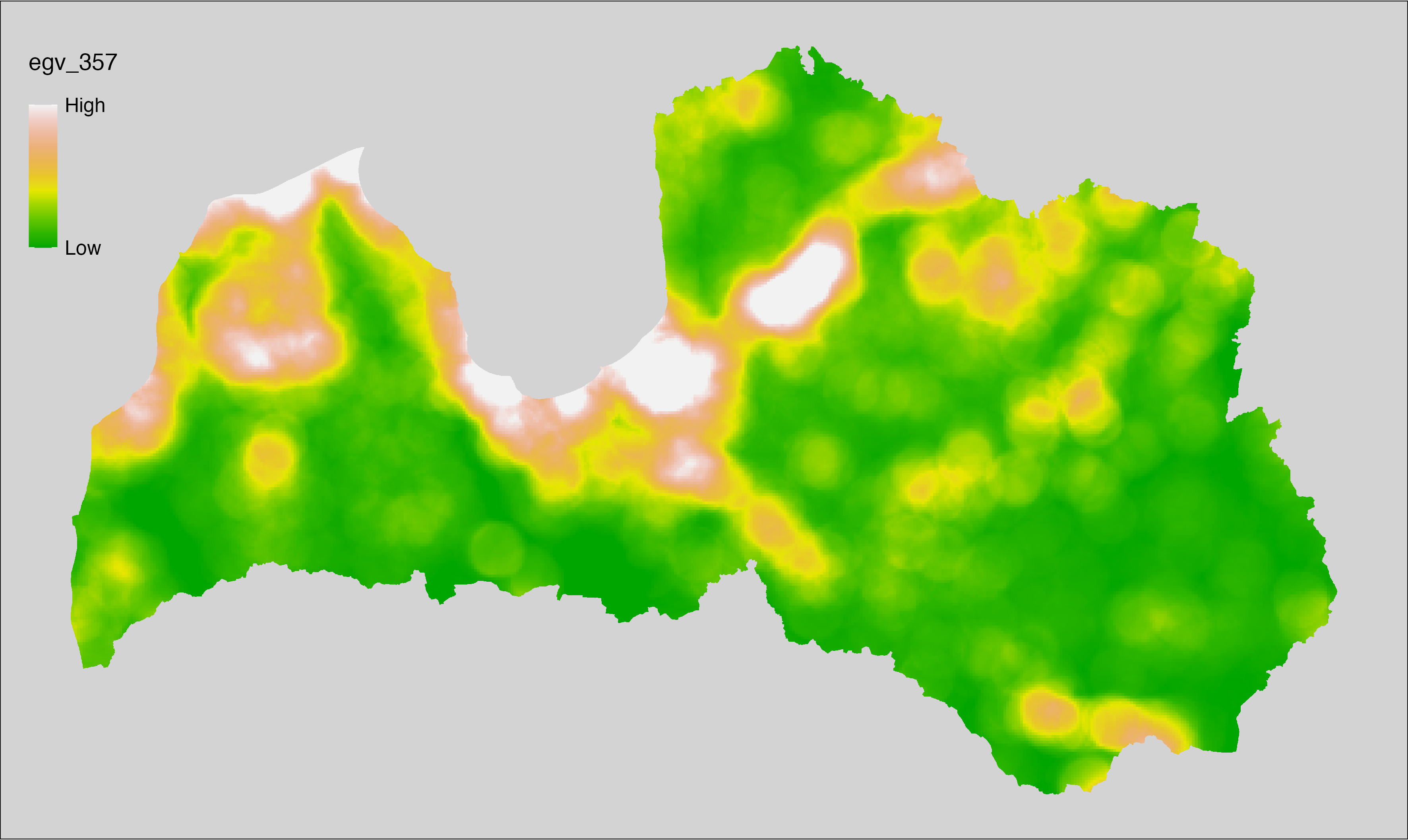
6.358 ForestsTreesAge_ConiferousYoung_cell
filename: ForestsTreesAge_ConiferousYoung_cell.tif
layername: egv_358
English name: Fractional cover of Young (pre-rotation age) Coniferous Forests within the analysis cell (1 ha)
Latvian name: Jaunu (pirms cirtmeta) skujkoku mežu platības īpatsvars analīzes šūnā (1 ha)
Procedure: Most EGVs describing forests are spatially restricted to areas outside of clearcuts and dead stands. This mask is created using a combination of the State Forest Service’s State Forest Registry land category 12 and 14, and The Global Forest Watch pixels classified as lost tree canopy cover since 2020 (raster layer matching input, presence = 1, absence = 0).
To prepare this EGV, stands from the State Forest Service’s State Forest Registry are classified into (in order):
coniferous (see Terminology and acronyms for species codes) if timber volume of those species exceeded 75%;
Boreal deciduous if timber volume of those species exceeded 75%;
temperate deciduous if timber volume of those species exceeded 50%;
mixed otherwise;
then coniferous stands younger than the legal rotation age are selected and
geometries are rasterised (presence = 1, NA otherwise). Rasterisation is
performed using the workflow egvtools::polygon2input(), restricting to pixels outside clearcut
mask and covering background with value 0. The resulting layer
is then aggregated to EGV resolution using the workflow egvtools::input2egv(), which
calculates the arithmetic mean to determine the cover fraction. During
aggregation, inverse distance weighted (power = 2) gap filling on the output is
applied to ensure no missing values at the edges. Finally, the layer is
standardised by subtracting the arithmetic mean and dividing by the root mean squared
error.
Code
# libs ----
if(!require(egvtools)) {remotes::install_github("aavotins/egvtools"); require(egvtools)}
if(!require(terra)) {install.packages("terra"); require(terra)}
if(!require(sf)) {install.packages("sf"); require(sf)}
if(!require(tidyverse)) {install.packages("tidyverse"); require(tidyverse)}
if(!require(sfarrow)) {install.packages("sfarrow"); require(sfarrow)}
if(!require(readxl)) {install.packages("readxl"); require(readxl)}
if(!require(raster)) {install.packages("raster"); require(raster)}
if(!require(fasterize)) {install.packages("fasterize"); require(fasterize)}
# templates ----
template100=rast("./Templates/TemplateRasters/LV100m_10km.tif")
template10=rast("./Templates/TemplateRasters/LV10m_10km.tif")
rastrs10=raster(template10)
nulls10=rast("./Templates/TemplateRasters/nulls_LV10m_10km.tif")
nulls100=rast("./Templates/TemplateRasters/nulls_LV100m_10km.tif")
# simple landscape ----
simple_landscape=rast("RasterGrids_10m/2024/Ainava_vienk_mask.tif")
# mvr ----
mvr=st_read_parquet("./Geodata/2024/MVR/nogabali_2024janv.parquet")
mvr$yes=1
# clear cut mask ----
izcirtumi=mvr %>%
filter(zkat %in% c("12","14")) %>%
dplyr::select(yes)
r_izcirtumi_mvr=fasterize(izcirtumi,rastrs10,field="yes")
t_izcirtumi_mvr=rast(r_izcirtumi_mvr)
plot(t_izcirtumi_mvr)
tcl=rast("./Geodata/2024/Trees/GFW/TreeCoverLoss_v1_12.tif")
tcl2=ifel(tcl<20,0,1)
tclX=cover(tcl2,nulls10)
plot(tclX)
clearcut_mask=cover(t_izcirtumi_mvr,tclX,
filename="./RasterGrids_10m/2024/Mask_clearcuts.tif",
overwrite=TRUE)
plot(clearcut_mask)
rm(izcirtumi)
rm(r_izcirtumi_mvr)
rm(t_izcirtumi_mvr)
rm(tcl)
rm(tcl2)
rm(tclX)
# ForestsTreesAge_ConiferousYoung_cell.tif egv_358 ----
skujkoki=c("1","3","13","14","15","22","23","28") # 8
saurlapji=c("4","6","8","9","19","20","21","32","35","68") # 10
platlapji=c("10","11","12","16","17","18","24","25","26","27","28","29","50",
"61","62","63","64","65","66","67","69") # 21
mvr=mvr %>%
mutate(kraja_skujkoku=ifelse(s10 %in% skujkoki,v10,0)+
ifelse(s11 %in% skujkoki,v11,0)+ifelse(s12 %in% skujkoki,v12,0)+
ifelse(s13 %in% skujkoki,v13,0)+ifelse(s14 %in% skujkoki,v14,0),
kraja_saurlapju=ifelse(s10 %in% saurlapji,v10,0)+
ifelse(s11 %in% saurlapji,v11,0)+ifelse(s12 %in% saurlapji,v12,0)+
ifelse(s13 %in% saurlapji,v13,0)+ifelse(s14 %in% saurlapji,v14,0),
kraja_platlapju=ifelse(s10 %in% platlapji,v10,0)+
ifelse(s11 %in% platlapji,v11,0)+ifelse(s12 %in% platlapji,v12,0)+
ifelse(s13 %in% platlapji,v13,0)+ifelse(s14 %in% platlapji,v14,0)) %>%
mutate(kopeja_kraja=kraja_skujkoku+kraja_platlapju+kraja_saurlapju) %>%
mutate(tips=ifelse(kraja_skujkoku/kopeja_kraja>=0.75,"skujkoku",
ifelse(kraja_saurlapju/kopeja_kraja>=0.75,"saurlapju",
ifelse(kraja_platlapju/kopeja_kraja>0.5,"platlapju",
"jauktu koku"))))
nogabali=mvr %>%
filter(zkat=="10"&tips=="skujkoku"&(vgr=="1"|vgr=="2"|vgr=="3"))
p2i_rez=egvtools::polygon2input(vector_data = nogabali,
template_path = "./Templates/TemplateRasters/LV10m_10km.tif",
out_path = "./RasterGrids_10m/2024/",
file_name = "ForestsTreesAge_ConiferousYoung_input.tif",
value_field = "yes",
restrict_to = clearcut_mask,
restrict_values = 0,
prepare=FALSE,
background_raster = "./Templates/TemplateRasters/nulls_LV10m_10km.tif",
plot_result = TRUE)
p2i_rez
i2e_rez=egvtools::input2egv(input=paste0("./RasterGrids_10m/2024/",
"ForestsTreesAge_ConiferousYoung_input.tif"),
egv_template= "./Templates/TemplateRasters/LV100m_10km.tif",
summary_function = "average",
missing_job = "FillOutput",
outlocation = "./RasterGrids_100m/2024/RAW/",
outfilename = "ForestsTreesAge_ConiferousYoung_cell.tif",
layername = "egv_358",
idw_weight = 2,
plot_gaps = FALSE,plot_final = TRUE)
i2e_rez
rm(nogabali)
rm(p2i_rez)
rm(i2e_rez)
unlink("./RasterGrids_10m/2024/ForestsTreesAge_ConiferousYoung_input.tif")
# standardisation ----
if(!require(terra)) {install.packages("terra"); require(terra)}
if(!require(tidyverse)) {install.packages("tidyverse"); require(tidyverse)}
nosaukums="ForestsTreesAge_ConiferousYoung_cell.tif"
ielasisanas_cels=paste0("./RasterGrids_100m/2024/RAW/",nosaukums)
saglabasanas_cels=paste0("./RasterGrids_100m/2024/Scaled/",nosaukums)
slanis=rast(ielasisanas_cels)
videjais=global(slanis,fun="mean",na.rm=TRUE)
centrets=slanis-videjais[,1]
standartnovirze=terra::global(centrets,fun="rms",na.rm=TRUE)
merogots=centrets/standartnovirze[,1]
writeRaster(merogots,
filename=saglabasanas_cels,
overwrite=TRUE)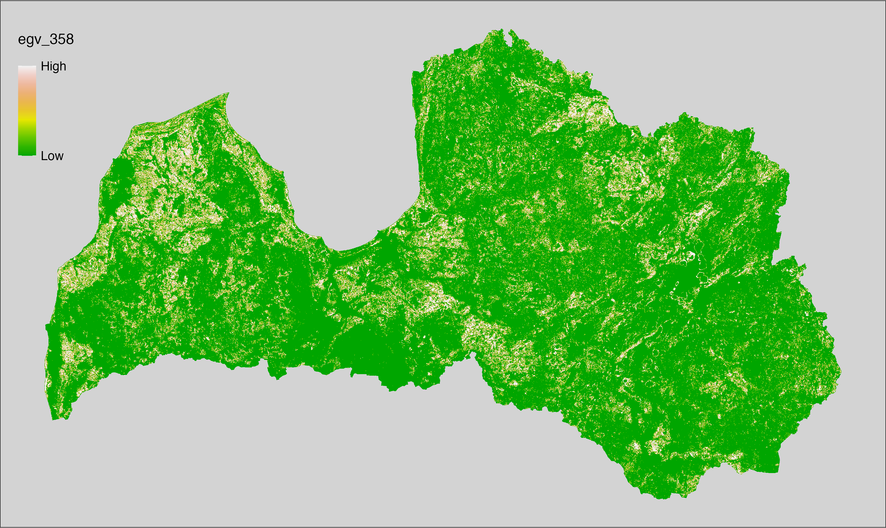
6.359 ForestsTreesAge_ConiferousYoung_r500
filename: ForestsTreesAge_ConiferousYoung_r500.tif
layername: egv_359
English name: Fractional cover of Young (pre-rotation age) Coniferous Forests within the 0.5 km landscape
Latvian name: Jaunu (pirms cirtmeta) skujkoku mežu platības īpatsvars 0,5 km ainavā
Procedure: The cover fraction within a radius of 500 m around the analysis grid cell is
calculated as the area-weighted sum of the analysis cells inside the
buffer, using the workflow egvtools::radius_function(). During the calculation of the landscape metric,
inverse distance weighted (power = 2) gap filling on the output is applied
to ensure no missing values at the edges. Then the layer is rewritten to set
its name. Finally, the layer is standardised by subtracting the arithmetic
mean and dividing by the root mean squared error.
Code
# libs ----
if(!require(terra)) {install.packages("terra"); require(terra)}
if(!require(egvtools)) {remotes::install_github("aavotins/egvtools"); require(egvtools)}
# Templates -----
template100=rast("./Templates/TemplateRasters/LV100m_10km.tif")
# radii ----
radius_function(
kvadrati_path = "./Templates/TemplateGrids/tiles/",
radii_path = "./Templates/TemplateGridPoints/tiles/",
tikls100_path = "./Templates/TemplateGrids/tikls100_sauzeme.parquet",
template_path = "./Templates/TemplateRasters/LV100m_10km.tif",
input_layers = c("./RasterGrids_100m/2024/RAW/ForestsTreesAge_ConiferousYoung_cell.tif"),
layer_prefixes = c("ForestsTreesAge_ConiferousYoung"),
output_dir = "./RasterGrids_100m/2024/RAW/",
n_workers = 6,
radii = c("r500"),
radius_mode = "sparse",
extract_fun = "mean",
fill_missing = TRUE,
IDW_weight = 2,
future_max_size = 40 * 1024^3)
# ForestsTreesAge_ConiferousYoung_r500.tif egv_359
slanis=rast("./RasterGrids_100m/2024/RAW/ForestsTreesAge_ConiferousYoung_r500.tif")
names(slanis)="egv_359"
slanis2=project(slanis,template100)
writeRaster(slanis2,
"./RasterGrids_100m/2024/RAW/ForestsTreesAge_ConiferousYoung_r500.tif",
overwrite=TRUE)
# standardisation ----
if(!require(terra)) {install.packages("terra"); require(terra)}
if(!require(tidyverse)) {install.packages("tidyverse"); require(tidyverse)}
nosaukums="ForestsTreesAge_ConiferousYoung_r500.tif"
ielasisanas_cels=paste0("./RasterGrids_100m/2024/RAW/",nosaukums)
saglabasanas_cels=paste0("./RasterGrids_100m/2024/Scaled/",nosaukums)
slanis=rast(ielasisanas_cels)
videjais=global(slanis,fun="mean",na.rm=TRUE)
centrets=slanis-videjais[,1]
standartnovirze=terra::global(centrets,fun="rms",na.rm=TRUE)
merogots=centrets/standartnovirze[,1]
writeRaster(merogots,
filename=saglabasanas_cels,
overwrite=TRUE)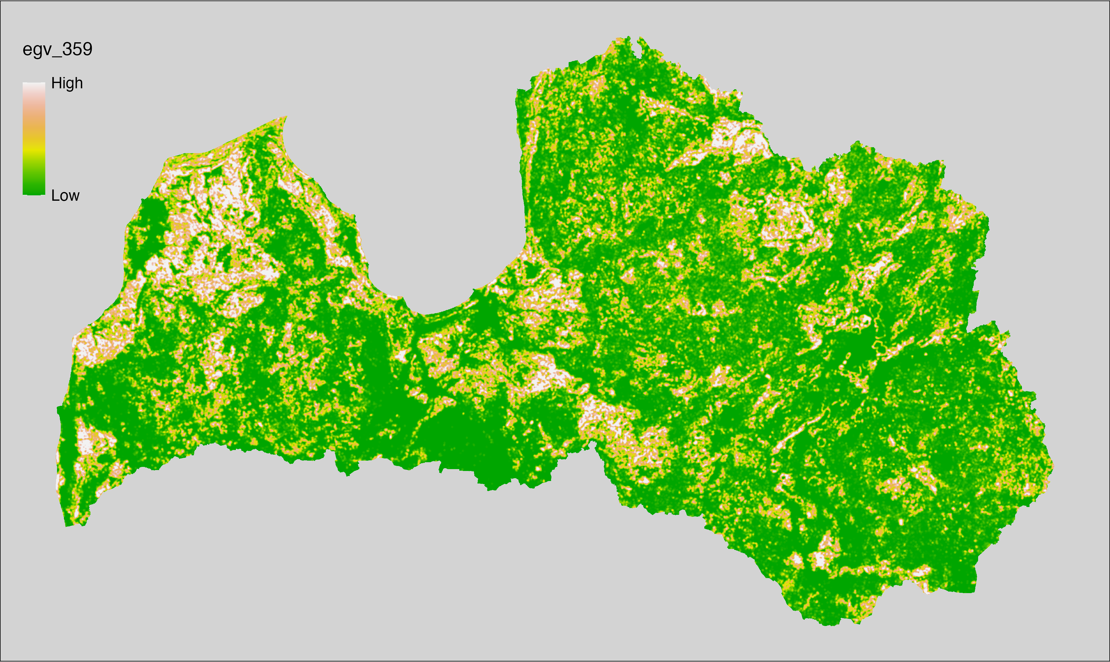
6.360 ForestsTreesAge_ConiferousYoung_r1250
filename: ForestsTreesAge_ConiferousYoung_r1250.tif
layername: egv_360
English name: Fractional cover of Young (pre-rotation age) Coniferous Forests within the 1.25 km landscape
Latvian name: Jaunu (pirms cirtmeta) skujkoku mežu platības īpatsvars 1,25 km ainavā
Procedure: The cover fraction within a radius of 1250 m around the analysis grid cell
is calculated as the area-weighted sum of the analysis cells inside
the buffer, using the workflow egvtools::radius_function(). During the calculation of the landscape
metric, inverse distance weighted (power = 2) gap filling on the output is
applied to ensure no missing values at the edges. Then the layer is
rewritten to set its name. Finally, the layer is standardised by
subtracting the arithmetic mean and dividing by the root mean squared error.
Code
# libs ----
if(!require(terra)) {install.packages("terra"); require(terra)}
if(!require(egvtools)) {remotes::install_github("aavotins/egvtools"); require(egvtools)}
# Templates -----
template100=rast("./Templates/TemplateRasters/LV100m_10km.tif")
# radii ----
radius_function(
kvadrati_path = "./Templates/TemplateGrids/tiles/",
radii_path = "./Templates/TemplateGridPoints/tiles/",
tikls100_path = "./Templates/TemplateGrids/tikls100_sauzeme.parquet",
template_path = "./Templates/TemplateRasters/LV100m_10km.tif",
input_layers = c("./RasterGrids_100m/2024/RAW/ForestsTreesAge_ConiferousYoung_cell.tif"),
layer_prefixes = c("ForestsTreesAge_ConiferousYoung"),
output_dir = "./RasterGrids_100m/2024/RAW/",
n_workers = 6,
radii = c("r1250"),
radius_mode = "sparse",
extract_fun = "mean",
fill_missing = TRUE,
IDW_weight = 2,
future_max_size = 40 * 1024^3)
# ForestsTreesAge_ConiferousYoung_r1250.tif egv_360
slanis=rast("./RasterGrids_100m/2024/RAW/ForestsTreesAge_ConiferousYoung_r1250.tif")
names(slanis)="egv_360"
slanis2=project(slanis,template100)
writeRaster(slanis2,
"./RasterGrids_100m/2024/RAW/ForestsTreesAge_ConiferousYoung_r1250.tif",
overwrite=TRUE)
# standardisation ----
if(!require(terra)) {install.packages("terra"); require(terra)}
if(!require(tidyverse)) {install.packages("tidyverse"); require(tidyverse)}
nosaukums="ForestsTreesAge_ConiferousYoung_r1250.tif"
ielasisanas_cels=paste0("./RasterGrids_100m/2024/RAW/",nosaukums)
saglabasanas_cels=paste0("./RasterGrids_100m/2024/Scaled/",nosaukums)
slanis=rast(ielasisanas_cels)
videjais=global(slanis,fun="mean",na.rm=TRUE)
centrets=slanis-videjais[,1]
standartnovirze=terra::global(centrets,fun="rms",na.rm=TRUE)
merogots=centrets/standartnovirze[,1]
writeRaster(merogots,
filename=saglabasanas_cels,
overwrite=TRUE)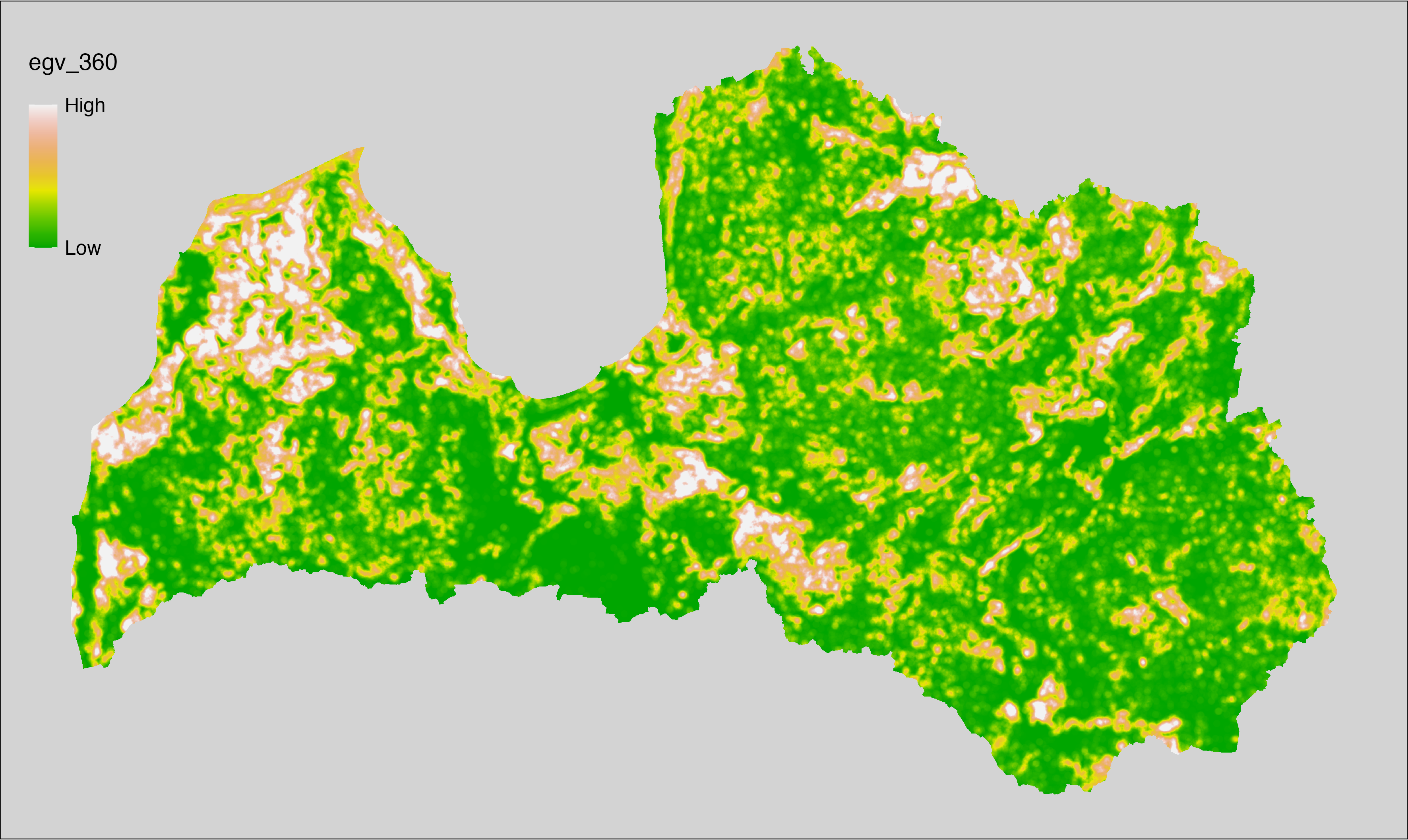
6.361 ForestsTreesAge_ConiferousYoung_r3000
filename: ForestsTreesAge_ConiferousYoung_r3000.tif
layername: egv_361
English name: Fractional cover of Young (pre-rotation age) Coniferous Forests within the 3 km landscape
Latvian name: Jaunu (pirms cirtmeta) skujkoku mežu platības īpatsvars 3 km ainavā
Procedure: The cover fraction within a radius of 3000 m around the analysis grid cell
is calculated as the area-weighted sum of the analysis cells inside
the buffer, using the workflow egvtools::radius_function(). During the calculation of the landscape
metric, inverse distance weighted (power = 2) gap filling on the output is
applied to ensure no missing values at the edges. Then the layer is
rewritten to set its name. Finally, the layer is standardised by
subtracting the arithmetic mean and dividing by the root mean squared error.
Code
# libs ----
if(!require(terra)) {install.packages("terra"); require(terra)}
if(!require(egvtools)) {remotes::install_github("aavotins/egvtools"); require(egvtools)}
# Templates -----
template100=rast("./Templates/TemplateRasters/LV100m_10km.tif")
# radii ----
radius_function(
kvadrati_path = "./Templates/TemplateGrids/tiles/",
radii_path = "./Templates/TemplateGridPoints/tiles/",
tikls100_path = "./Templates/TemplateGrids/tikls100_sauzeme.parquet",
template_path = "./Templates/TemplateRasters/LV100m_10km.tif",
input_layers = c("./RasterGrids_100m/2024/RAW/ForestsTreesAge_ConiferousYoung_cell.tif"),
layer_prefixes = c("ForestsTreesAge_ConiferousYoung"),
output_dir = "./RasterGrids_100m/2024/RAW/",
n_workers = 6,
radii = c("r3000"),
radius_mode = "sparse",
extract_fun = "mean",
fill_missing = TRUE,
IDW_weight = 2,
future_max_size = 40 * 1024^3)
# ForestsTreesAge_ConiferousYoung_r3000.tif egv_361
slanis=rast("./RasterGrids_100m/2024/RAW/ForestsTreesAge_ConiferousYoung_r3000.tif")
names(slanis)="egv_361"
slanis2=project(slanis,template100)
writeRaster(slanis2,
"./RasterGrids_100m/2024/RAW/ForestsTreesAge_ConiferousYoung_r3000.tif",
overwrite=TRUE)
# standardisation ----
if(!require(terra)) {install.packages("terra"); require(terra)}
if(!require(tidyverse)) {install.packages("tidyverse"); require(tidyverse)}
nosaukums="ForestsTreesAge_ConiferousYoung_r3000.tif"
ielasisanas_cels=paste0("./RasterGrids_100m/2024/RAW/",nosaukums)
saglabasanas_cels=paste0("./RasterGrids_100m/2024/Scaled/",nosaukums)
slanis=rast(ielasisanas_cels)
videjais=global(slanis,fun="mean",na.rm=TRUE)
centrets=slanis-videjais[,1]
standartnovirze=terra::global(centrets,fun="rms",na.rm=TRUE)
merogots=centrets/standartnovirze[,1]
writeRaster(merogots,
filename=saglabasanas_cels,
overwrite=TRUE)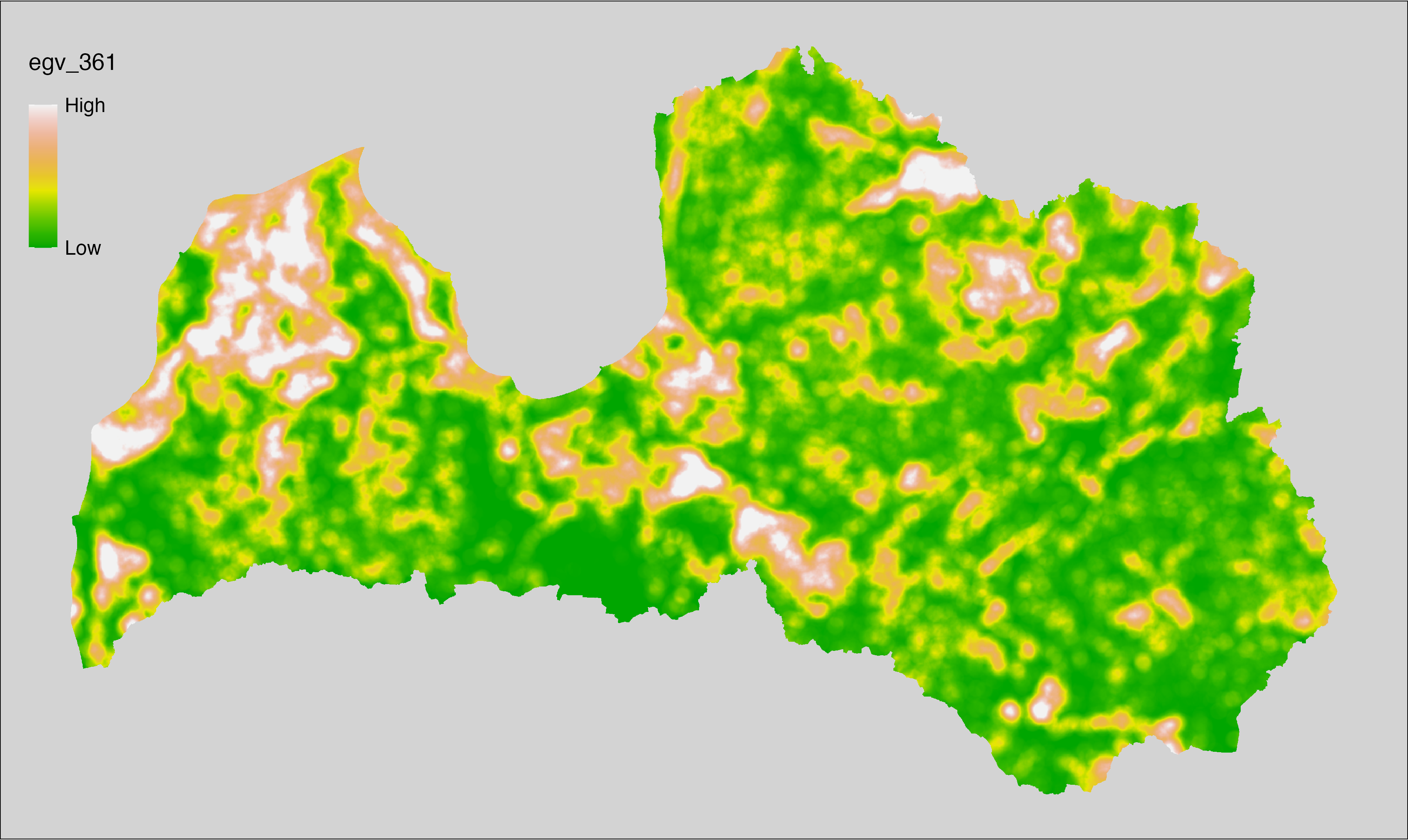
6.362 ForestsTreesAge_ConiferousYoung_r10000
filename: ForestsTreesAge_ConiferousYoung_r10000.tif
layername: egv_362
English name: Fractional cover of Young (pre-rotation age) Coniferous Forests within the 10 km landscape
Latvian name: Jaunu (pirms cirtmeta) skujkoku mežu platības īpatsvars 10 km ainavā
Procedure: The cover fraction within a radius of 10000 m around the analysis grid cell
is calculated as the area-weighted sum of the analysis cells inside
the buffer, using the workflow egvtools::radius_function(). During the calculation of the landscape
metric, inverse distance weighted (power = 2) gap filling on the output is
applied to ensure no missing values at the edges. Then the layer is
rewritten to set its name. Finally, the layer is standardised by
subtracting the arithmetic mean and dividing by the root mean squared error.
Code
# libs ----
if(!require(terra)) {install.packages("terra"); require(terra)}
if(!require(egvtools)) {remotes::install_github("aavotins/egvtools"); require(egvtools)}
# Templates -----
template100=rast("./Templates/TemplateRasters/LV100m_10km.tif")
# radii ----
radius_function(
kvadrati_path = "./Templates/TemplateGrids/tiles/",
radii_path = "./Templates/TemplateGridPoints/tiles/",
tikls100_path = "./Templates/TemplateGrids/tikls100_sauzeme.parquet",
template_path = "./Templates/TemplateRasters/LV100m_10km.tif",
input_layers = c("./RasterGrids_100m/2024/RAW/ForestsTreesAge_ConiferousYoung_cell.tif"),
layer_prefixes = c("ForestsTreesAge_ConiferousYoung"),
output_dir = "./RasterGrids_100m/2024/RAW/",
n_workers = 6,
radii = c("r10000"),
radius_mode = "sparse",
extract_fun = "mean",
fill_missing = TRUE,
IDW_weight = 2,
future_max_size = 40 * 1024^3)
# ForestsTreesAge_ConiferousYoung_r10000.tif egv_362
slanis=rast("./RasterGrids_100m/2024/RAW/ForestsTreesAge_ConiferousYoung_r10000.tif")
names(slanis)="egv_362"
slanis2=project(slanis,template100)
writeRaster(slanis2,
"./RasterGrids_100m/2024/RAW/ForestsTreesAge_ConiferousYoung_r10000.tif",
overwrite=TRUE)
# standardisation ----
if(!require(terra)) {install.packages("terra"); require(terra)}
if(!require(tidyverse)) {install.packages("tidyverse"); require(tidyverse)}
nosaukums="ForestsTreesAge_ConiferousYoung_r10000.tif"
ielasisanas_cels=paste0("./RasterGrids_100m/2024/RAW/",nosaukums)
saglabasanas_cels=paste0("./RasterGrids_100m/2024/Scaled/",nosaukums)
slanis=rast(ielasisanas_cels)
videjais=global(slanis,fun="mean",na.rm=TRUE)
centrets=slanis-videjais[,1]
standartnovirze=terra::global(centrets,fun="rms",na.rm=TRUE)
merogots=centrets/standartnovirze[,1]
writeRaster(merogots,
filename=saglabasanas_cels,
overwrite=TRUE)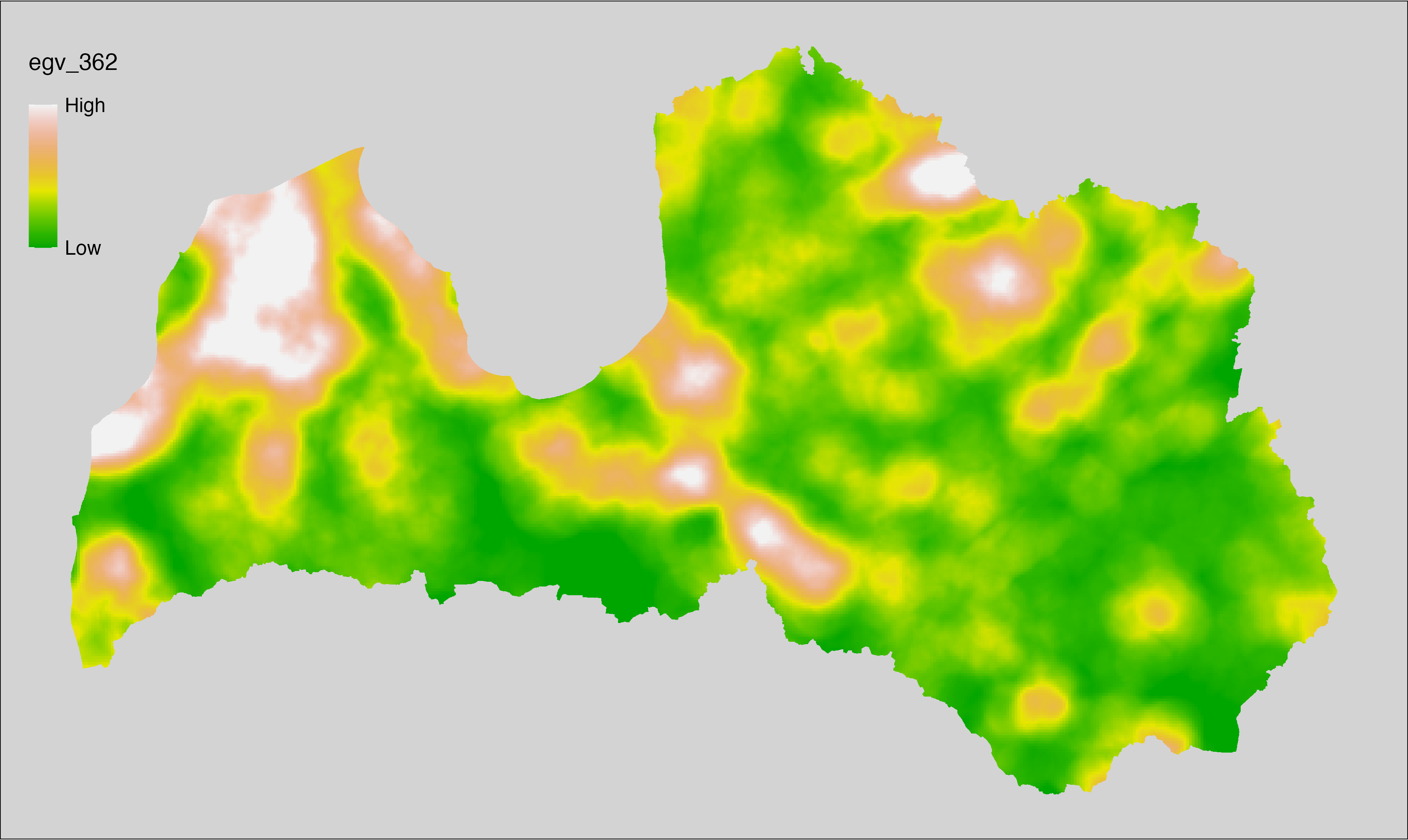
6.363 ForestsTreesAge_MixedOld_cell
filename: ForestsTreesAge_MixedOld_cell.tif
layername: egv_363
English name: Fractional cover of Old (over rotation age) Mixed Forests within the analysis cell (1 ha)
Latvian name: Vecu (kopš cirtmeta) jauktu koku mežu platības īpatsvars analīzes šūnā (1 ha)
Procedure: Most EGVs describing forests are spatially restricted to areas outside of clearcuts and dead stands. This mask is created using a combination of the State Forest Service’s State Forest Registry land category 12 and 14, and The Global Forest Watch pixels classified as lost tree canopy cover since 2020 (raster layer matching input, presence = 1, absence = 0).
To prepare this EGV, stands from the State Forest Service’s State Forest Registry are classified into (in order):
coniferous (see Terminology and acronyms for species codes) if timber volume of those species exceeded 75%;
Boreal deciduous if timber volume of those species exceeded 75%;
temperate deciduous if timber volume of those species exceeded 50%;
mixed otherwise;
then mixed stands exceeding the legal rotation age are selected and
geometries are rasterised (presence = 1, NA otherwise). Rasterisation is
performed using the workflow egvtools::polygon2input(), restricting to pixels outside clearcut
mask and covering background with value 0. The resulting layer
is then aggregated to EGV resolution using the workflow egvtools::input2egv(), which
calculates the arithmetic mean to determine the cover fraction. During
aggregation, inverse distance weighted (power = 2) gap filling on the output is
applied to ensure no missing values at the edges. Finally, the layer is
standardised by subtracting the arithmetic mean and dividing by the root mean squared
error.
Code
# libs ----
if(!require(egvtools)) {remotes::install_github("aavotins/egvtools"); require(egvtools)}
if(!require(terra)) {install.packages("terra"); require(terra)}
if(!require(sf)) {install.packages("sf"); require(sf)}
if(!require(tidyverse)) {install.packages("tidyverse"); require(tidyverse)}
if(!require(sfarrow)) {install.packages("sfarrow"); require(sfarrow)}
if(!require(readxl)) {install.packages("readxl"); require(readxl)}
if(!require(raster)) {install.packages("raster"); require(raster)}
if(!require(fasterize)) {install.packages("fasterize"); require(fasterize)}
# templates ----
template100=rast("./Templates/TemplateRasters/LV100m_10km.tif")
template10=rast("./Templates/TemplateRasters/LV10m_10km.tif")
rastrs10=raster(template10)
nulls10=rast("./Templates/TemplateRasters/nulls_LV10m_10km.tif")
nulls100=rast("./Templates/TemplateRasters/nulls_LV100m_10km.tif")
# simple landscape ----
simple_landscape=rast("RasterGrids_10m/2024/Ainava_vienk_mask.tif")
# mvr ----
mvr=st_read_parquet("./Geodata/2024/MVR/nogabali_2024janv.parquet")
mvr$yes=1
# clear cut mask ----
izcirtumi=mvr %>%
filter(zkat %in% c("12","14")) %>%
dplyr::select(yes)
r_izcirtumi_mvr=fasterize(izcirtumi,rastrs10,field="yes")
t_izcirtumi_mvr=rast(r_izcirtumi_mvr)
plot(t_izcirtumi_mvr)
tcl=rast("./Geodata/2024/Trees/GFW/TreeCoverLoss_v1_12.tif")
tcl2=ifel(tcl<20,0,1)
tclX=cover(tcl2,nulls10)
plot(tclX)
clearcut_mask=cover(t_izcirtumi_mvr,tclX,
filename="./RasterGrids_10m/2024/Mask_clearcuts.tif",
overwrite=TRUE)
plot(clearcut_mask)
rm(izcirtumi)
rm(r_izcirtumi_mvr)
rm(t_izcirtumi_mvr)
rm(tcl)
rm(tcl2)
rm(tclX)
# ForestsTreesAge_MixedOld_cell.tif egv_363 ----
skujkoki=c("1","3","13","14","15","22","23","28") # 8
saurlapji=c("4","6","8","9","19","20","21","32","35","68") # 10
platlapji=c("10","11","12","16","17","18","24","25","26","27","28","29","50",
"61","62","63","64","65","66","67","69") # 21
mvr=mvr %>%
mutate(kraja_skujkoku=ifelse(s10 %in% skujkoki,v10,0)+
ifelse(s11 %in% skujkoki,v11,0)+ifelse(s12 %in% skujkoki,v12,0)+
ifelse(s13 %in% skujkoki,v13,0)+ifelse(s14 %in% skujkoki,v14,0),
kraja_saurlapju=ifelse(s10 %in% saurlapji,v10,0)+
ifelse(s11 %in% saurlapji,v11,0)+ifelse(s12 %in% saurlapji,v12,0)+
ifelse(s13 %in% saurlapji,v13,0)+ifelse(s14 %in% saurlapji,v14,0),
kraja_platlapju=ifelse(s10 %in% platlapji,v10,0)+
ifelse(s11 %in% platlapji,v11,0)+ifelse(s12 %in% platlapji,v12,0)+
ifelse(s13 %in% platlapji,v13,0)+ifelse(s14 %in% platlapji,v14,0)) %>%
mutate(kopeja_kraja=kraja_skujkoku+kraja_platlapju+kraja_saurlapju) %>%
mutate(tips=ifelse(kraja_skujkoku/kopeja_kraja>=0.75,"skujkoku",
ifelse(kraja_saurlapju/kopeja_kraja>=0.75,"saurlapju",
ifelse(kraja_platlapju/kopeja_kraja>0.5,"platlapju",
"jauktu koku"))))
nogabali=mvr %>%
filter(zkat=="10"&tips=="jauktu koku"&(vgr=="4"|vgr=="5"))
p2i_rez=egvtools::polygon2input(vector_data = nogabali,
template_path = "./Templates/TemplateRasters/LV10m_10km.tif",
out_path = "./RasterGrids_10m/2024/",
file_name = "ForestsTreesAge_MixedOld_input.tif",
value_field = "yes",
restrict_to = clearcut_mask,
restrict_values = 0,
prepare=FALSE,
background_raster = "./Templates/TemplateRasters/nulls_LV10m_10km.tif",
plot_result = TRUE)
p2i_rez
i2e_rez=egvtools::input2egv(input=paste0("./RasterGrids_10m/2024/",
"ForestsTreesAge_MixedOld_input.tif"),
egv_template= "./Templates/TemplateRasters/LV100m_10km.tif",
summary_function = "average",
missing_job = "FillOutput",
outlocation = "./RasterGrids_100m/2024/RAW/",
outfilename = "ForestsTreesAge_MixedOld_cell.tif",
layername = "egv_363",
idw_weight = 2,
plot_gaps = FALSE,plot_final = TRUE)
i2e_rez
rm(nogabali)
rm(p2i_rez)
rm(i2e_rez)
unlink("./RasterGrids_10m/2024/ForestsTreesAge_MixedOld_input.tif")
# standardisation ----
if(!require(terra)) {install.packages("terra"); require(terra)}
if(!require(tidyverse)) {install.packages("tidyverse"); require(tidyverse)}
nosaukums="ForestsTreesAge_MixedOld_cell.tif"
ielasisanas_cels=paste0("./RasterGrids_100m/2024/RAW/",nosaukums)
saglabasanas_cels=paste0("./RasterGrids_100m/2024/Scaled/",nosaukums)
slanis=rast(ielasisanas_cels)
videjais=global(slanis,fun="mean",na.rm=TRUE)
centrets=slanis-videjais[,1]
standartnovirze=terra::global(centrets,fun="rms",na.rm=TRUE)
merogots=centrets/standartnovirze[,1]
writeRaster(merogots,
filename=saglabasanas_cels,
overwrite=TRUE)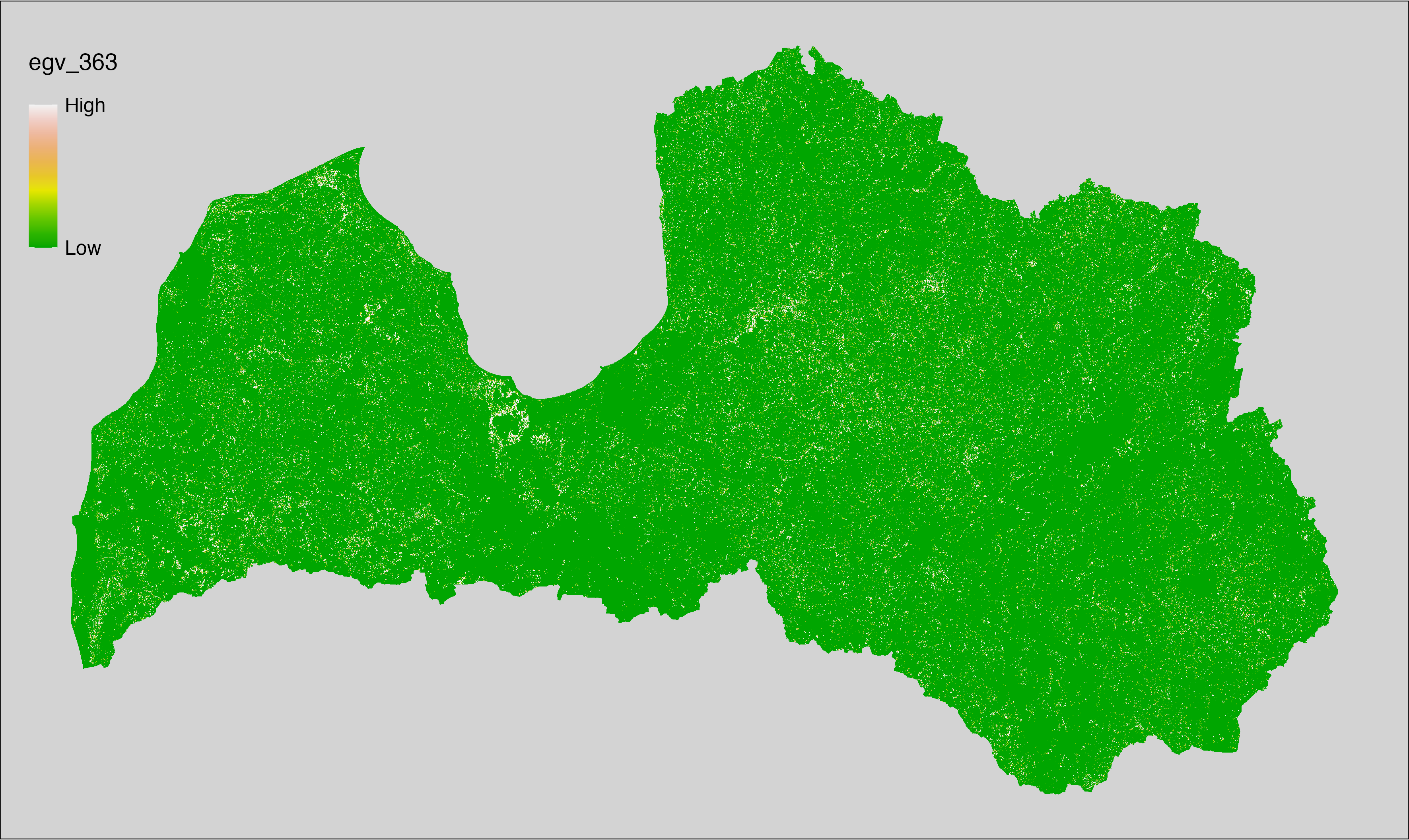
6.364 ForestsTreesAge_MixedOld_r500
filename: ForestsTreesAge_MixedOld_r500.tif
layername: egv_364
English name: Fractional cover of Old (over rotation age) Mixed Forests within the 0.5 km landscape
Latvian name: Vecu (kopš cirtmeta) jauktu koku mežu platības īpatsvars 0,5 km ainavā
Procedure: The cover fraction within a radius of 500 m around the analysis grid cell is
calculated as the area-weighted sum of the analysis cells inside the
buffer, using the workflow egvtools::radius_function(). During the calculation of the landscape metric,
inverse distance weighted (power = 2) gap filling on the output is applied
to ensure no missing values at the edges. Then the layer is rewritten to set
its name. Finally, the layer is standardised by subtracting the arithmetic
mean and dividing by the root mean squared error.
Code
# libs ----
if(!require(terra)) {install.packages("terra"); require(terra)}
if(!require(egvtools)) {remotes::install_github("aavotins/egvtools"); require(egvtools)}
# Templates -----
template100=rast("./Templates/TemplateRasters/LV100m_10km.tif")
# radii ----
radius_function(
kvadrati_path = "./Templates/TemplateGrids/tiles/",
radii_path = "./Templates/TemplateGridPoints/tiles/",
tikls100_path = "./Templates/TemplateGrids/tikls100_sauzeme.parquet",
template_path = "./Templates/TemplateRasters/LV100m_10km.tif",
input_layers = c("./RasterGrids_100m/2024/RAW/ForestsTreesAge_MixedOld_cell.tif"),
layer_prefixes = c("ForestsTreesAge_MixedOld"),
output_dir = "./RasterGrids_100m/2024/RAW/",
n_workers = 6,
radii = c("r500"),
radius_mode = "sparse",
extract_fun = "mean",
fill_missing = TRUE,
IDW_weight = 2,
future_max_size = 40 * 1024^3)
# ForestsTreesAge_MixedOld_r500.tif egv_364
slanis=rast("./RasterGrids_100m/2024/RAW/ForestsTreesAge_MixedOld_r500.tif")
names(slanis)="egv_364"
slanis2=project(slanis,template100)
writeRaster(slanis2,
"./RasterGrids_100m/2024/RAW/ForestsTreesAge_MixedOld_r500.tif",
overwrite=TRUE)
# standardisation ----
if(!require(terra)) {install.packages("terra"); require(terra)}
if(!require(tidyverse)) {install.packages("tidyverse"); require(tidyverse)}
nosaukums="ForestsTreesAge_MixedOld_r500.tif"
ielasisanas_cels=paste0("./RasterGrids_100m/2024/RAW/",nosaukums)
saglabasanas_cels=paste0("./RasterGrids_100m/2024/Scaled/",nosaukums)
slanis=rast(ielasisanas_cels)
videjais=global(slanis,fun="mean",na.rm=TRUE)
centrets=slanis-videjais[,1]
standartnovirze=terra::global(centrets,fun="rms",na.rm=TRUE)
merogots=centrets/standartnovirze[,1]
writeRaster(merogots,
filename=saglabasanas_cels,
overwrite=TRUE)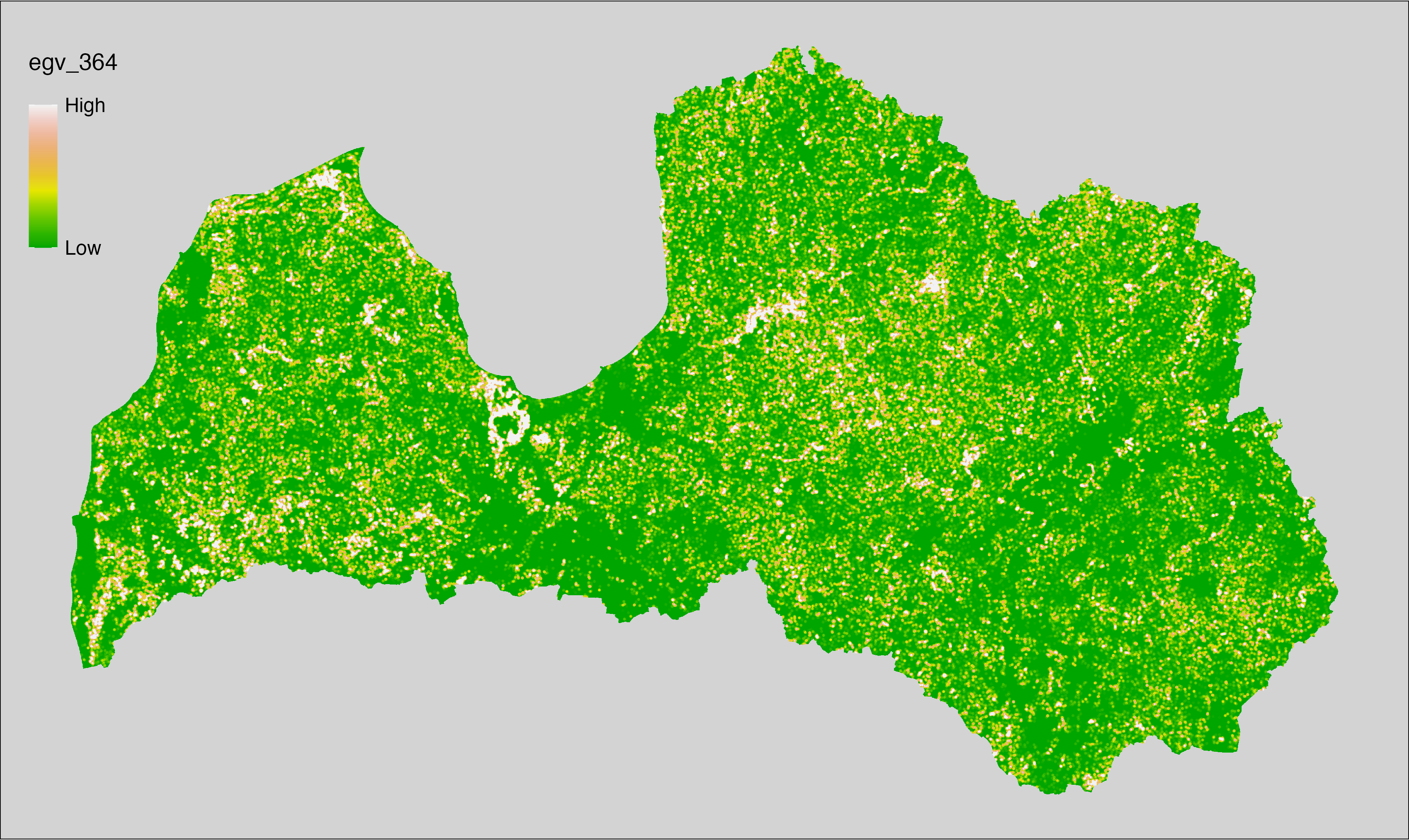
6.365 ForestsTreesAge_MixedOld_r1250
filename: ForestsTreesAge_MixedOld_r1250.tif
layername: egv_365
English name: Fractional cover of Old (over rotation age) Mixed Forests within the 1.25 km landscape
Latvian name: Vecu (kopš cirtmeta) jauktu koku mežu platības īpatsvars 1,25 km ainavā
Procedure: The cover fraction within a radius of 1250 m around the analysis grid cell
is calculated as the area-weighted sum of the analysis cells inside
the buffer, using the workflow egvtools::radius_function(). During the calculation of the landscape
metric, inverse distance weighted (power = 2) gap filling on the output is
applied to ensure no missing values at the edges. Then the layer is
rewritten to set its name. Finally, the layer is standardised by
subtracting the arithmetic mean and dividing by the root mean squared error.
Code
# libs ----
if(!require(terra)) {install.packages("terra"); require(terra)}
if(!require(egvtools)) {remotes::install_github("aavotins/egvtools"); require(egvtools)}
# Templates -----
template100=rast("./Templates/TemplateRasters/LV100m_10km.tif")
# radii ----
radius_function(
kvadrati_path = "./Templates/TemplateGrids/tiles/",
radii_path = "./Templates/TemplateGridPoints/tiles/",
tikls100_path = "./Templates/TemplateGrids/tikls100_sauzeme.parquet",
template_path = "./Templates/TemplateRasters/LV100m_10km.tif",
input_layers = c("./RasterGrids_100m/2024/RAW/ForestsTreesAge_MixedOld_cell.tif"),
layer_prefixes = c("ForestsTreesAge_MixedOld"),
output_dir = "./RasterGrids_100m/2024/RAW/",
n_workers = 6,
radii = c("r1250"),
radius_mode = "sparse",
extract_fun = "mean",
fill_missing = TRUE,
IDW_weight = 2,
future_max_size = 40 * 1024^3)
# ForestsTreesAge_MixedOld_r1250.tif egv_365
slanis=rast("./RasterGrids_100m/2024/RAW/ForestsTreesAge_MixedOld_r1250.tif")
names(slanis)="egv_365"
slanis2=project(slanis,template100)
writeRaster(slanis2,
"./RasterGrids_100m/2024/RAW/ForestsTreesAge_MixedOld_r1250.tif",
overwrite=TRUE)
# standardisation ----
if(!require(terra)) {install.packages("terra"); require(terra)}
if(!require(tidyverse)) {install.packages("tidyverse"); require(tidyverse)}
nosaukums="ForestsTreesAge_MixedOld_r1250.tif"
ielasisanas_cels=paste0("./RasterGrids_100m/2024/RAW/",nosaukums)
saglabasanas_cels=paste0("./RasterGrids_100m/2024/Scaled/",nosaukums)
slanis=rast(ielasisanas_cels)
videjais=global(slanis,fun="mean",na.rm=TRUE)
centrets=slanis-videjais[,1]
standartnovirze=terra::global(centrets,fun="rms",na.rm=TRUE)
merogots=centrets/standartnovirze[,1]
writeRaster(merogots,
filename=saglabasanas_cels,
overwrite=TRUE)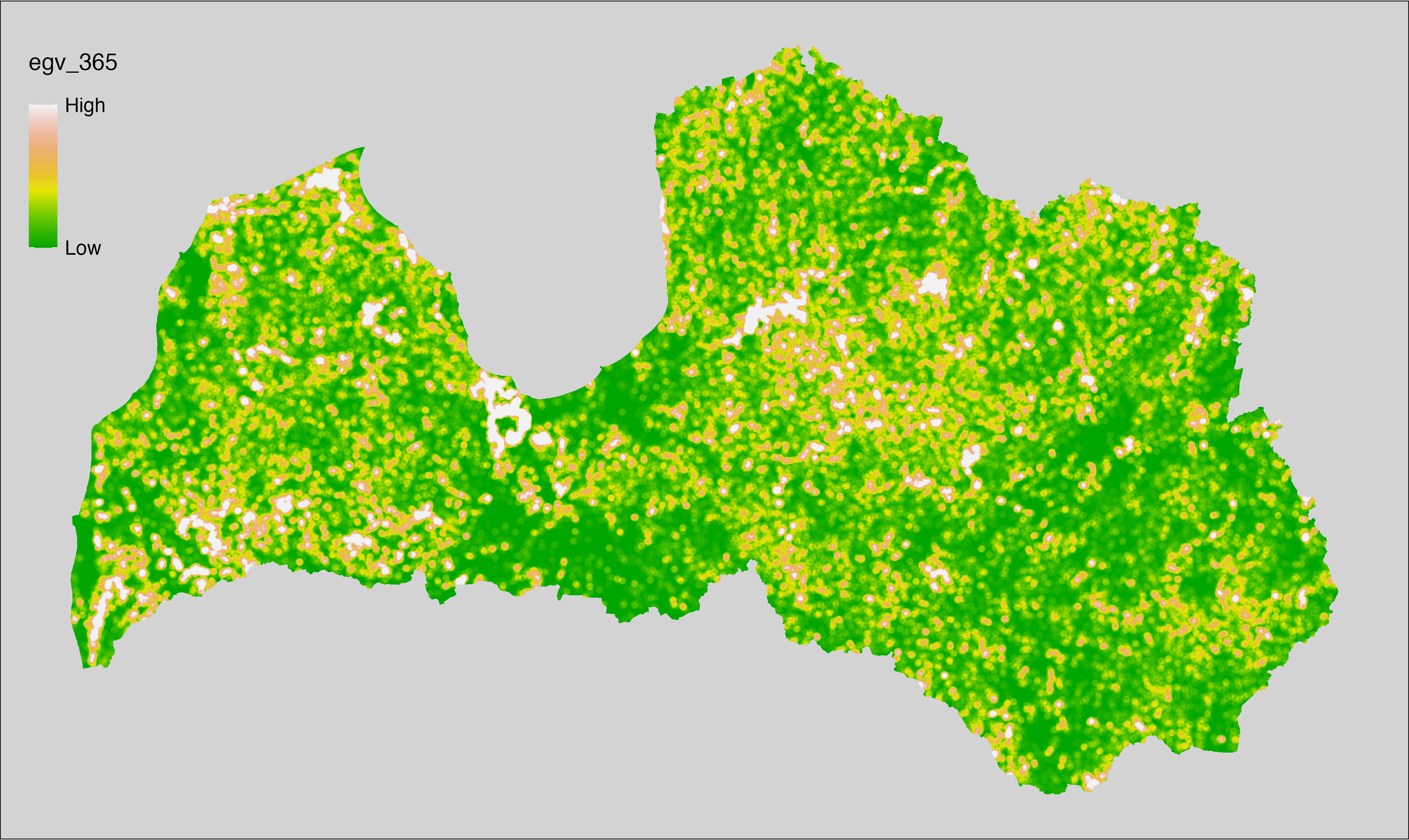
6.366 ForestsTreesAge_MixedOld_r3000
filename: ForestsTreesAge_MixedOld_r3000.tif
layername: egv_366
English name: Fractional cover of Old (over rotation age) Mixed Forests within the 3 km landscape
Latvian name: Vecu (kopš cirtmeta) jauktu koku mežu platības īpatsvars 3 km ainavā
Procedure: The cover fraction within a radius of 3000 m around the analysis grid cell
is calculated as the area-weighted sum of the analysis cells inside
the buffer, using the workflow egvtools::radius_function(). During the calculation of the landscape
metric, inverse distance weighted (power = 2) gap filling on the output is
applied to ensure no missing values at the edges. Then the layer is
rewritten to set its name. Finally, the layer is standardised by
subtracting the arithmetic mean and dividing by the root mean squared error.
Code
# libs ----
if(!require(terra)) {install.packages("terra"); require(terra)}
if(!require(egvtools)) {remotes::install_github("aavotins/egvtools"); require(egvtools)}
# Templates -----
template100=rast("./Templates/TemplateRasters/LV100m_10km.tif")
# radii ----
radius_function(
kvadrati_path = "./Templates/TemplateGrids/tiles/",
radii_path = "./Templates/TemplateGridPoints/tiles/",
tikls100_path = "./Templates/TemplateGrids/tikls100_sauzeme.parquet",
template_path = "./Templates/TemplateRasters/LV100m_10km.tif",
input_layers = c("./RasterGrids_100m/2024/RAW/ForestsTreesAge_MixedOld_cell.tif"),
layer_prefixes = c("ForestsTreesAge_MixedOld"),
output_dir = "./RasterGrids_100m/2024/RAW/",
n_workers = 6,
radii = c("r3000"),
radius_mode = "sparse",
extract_fun = "mean",
fill_missing = TRUE,
IDW_weight = 2,
future_max_size = 40 * 1024^3)
# ForestsTreesAge_MixedOld_r3000.tif egv_366
slanis=rast("./RasterGrids_100m/2024/RAW/ForestsTreesAge_MixedOld_r3000.tif")
names(slanis)="egv_366"
slanis2=project(slanis,template100)
writeRaster(slanis2,
"./RasterGrids_100m/2024/RAW/ForestsTreesAge_MixedOld_r3000.tif",
overwrite=TRUE)
# standardisation ----
if(!require(terra)) {install.packages("terra"); require(terra)}
if(!require(tidyverse)) {install.packages("tidyverse"); require(tidyverse)}
nosaukums="ForestsTreesAge_MixedOld_r3000.tif"
ielasisanas_cels=paste0("./RasterGrids_100m/2024/RAW/",nosaukums)
saglabasanas_cels=paste0("./RasterGrids_100m/2024/Scaled/",nosaukums)
slanis=rast(ielasisanas_cels)
videjais=global(slanis,fun="mean",na.rm=TRUE)
centrets=slanis-videjais[,1]
standartnovirze=terra::global(centrets,fun="rms",na.rm=TRUE)
merogots=centrets/standartnovirze[,1]
writeRaster(merogots,
filename=saglabasanas_cels,
overwrite=TRUE)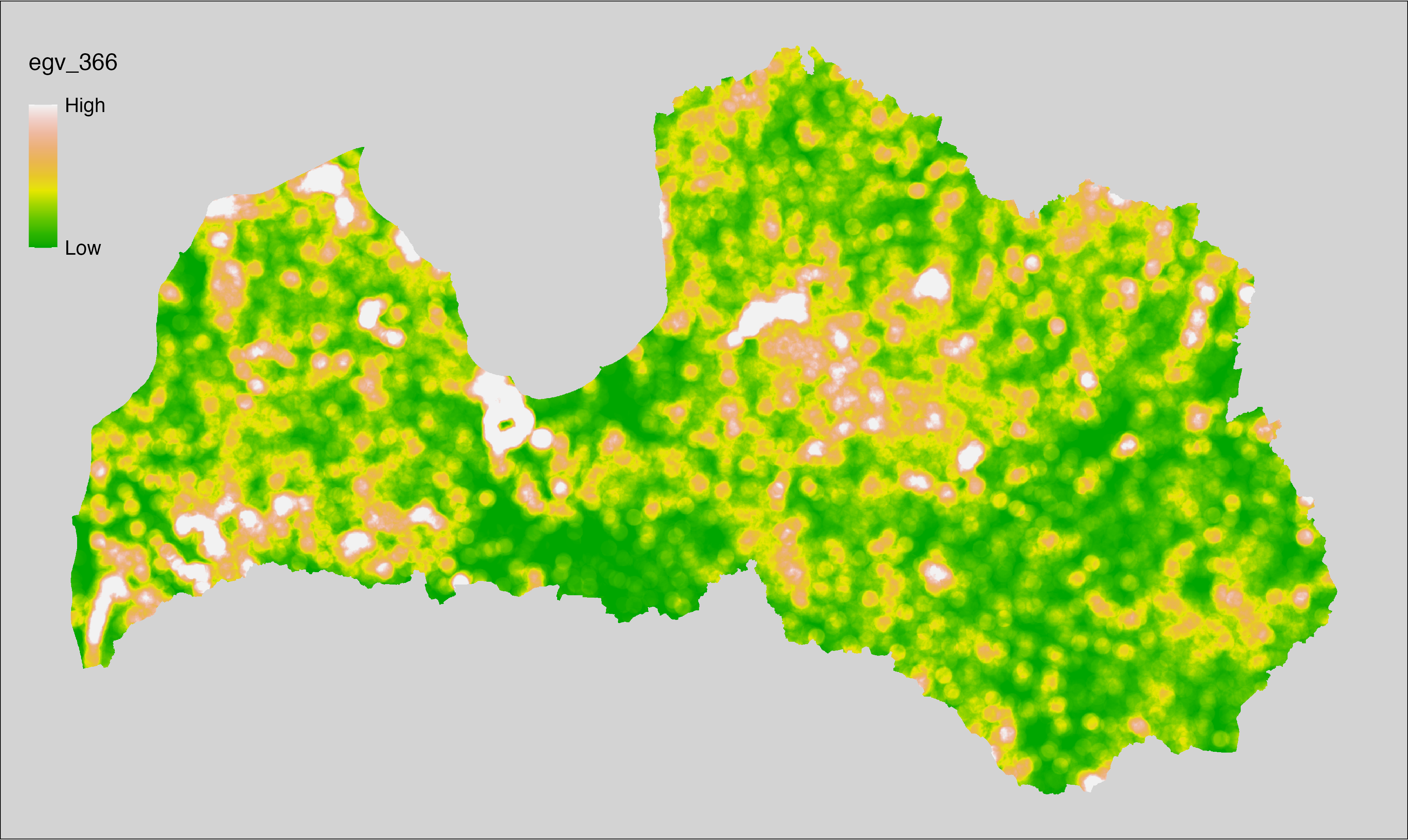
6.367 ForestsTreesAge_MixedOld_r10000
filename: ForestsTreesAge_MixedOld_r10000.tif
layername: egv_367
English name: Fractional cover of Old (over rotation age) Mixed Forests within the 10 km landscape
Latvian name: Vecu (kopš cirtmeta) jauktu koku mežu platības īpatsvars 10 km ainavā
Procedure: The cover fraction within a radius of 10000 m around the analysis grid cell
is calculated as the area-weighted sum of the analysis cells inside
the buffer, using the workflow egvtools::radius_function(). During the calculation of the landscape
metric, inverse distance weighted (power = 2) gap filling on the output is
applied to ensure no missing values at the edges. Then the layer is
rewritten to set its name. Finally, the layer is standardised by
subtracting the arithmetic mean and dividing by the root mean squared error.
Code
# libs ----
if(!require(terra)) {install.packages("terra"); require(terra)}
if(!require(egvtools)) {remotes::install_github("aavotins/egvtools"); require(egvtools)}
# Templates -----
template100=rast("./Templates/TemplateRasters/LV100m_10km.tif")
# radii ----
radius_function(
kvadrati_path = "./Templates/TemplateGrids/tiles/",
radii_path = "./Templates/TemplateGridPoints/tiles/",
tikls100_path = "./Templates/TemplateGrids/tikls100_sauzeme.parquet",
template_path = "./Templates/TemplateRasters/LV100m_10km.tif",
input_layers = c("./RasterGrids_100m/2024/RAW/ForestsTreesAge_MixedOld_cell.tif"),
layer_prefixes = c("ForestsTreesAge_MixedOld"),
output_dir = "./RasterGrids_100m/2024/RAW/",
n_workers = 6,
radii = c("r10000"),
radius_mode = "sparse",
extract_fun = "mean",
fill_missing = TRUE,
IDW_weight = 2,
future_max_size = 40 * 1024^3)
# ForestsTreesAge_MixedOld_r10000.tif egv_367
slanis=rast("./RasterGrids_100m/2024/RAW/ForestsTreesAge_MixedOld_r10000.tif")
names(slanis)="egv_367"
slanis2=project(slanis,template100)
writeRaster(slanis2,
"./RasterGrids_100m/2024/RAW/ForestsTreesAge_MixedOld_r10000.tif",
overwrite=TRUE)
# standardisation ----
if(!require(terra)) {install.packages("terra"); require(terra)}
if(!require(tidyverse)) {install.packages("tidyverse"); require(tidyverse)}
nosaukums="ForestsTreesAge_MixedOld_r10000.tif"
ielasisanas_cels=paste0("./RasterGrids_100m/2024/RAW/",nosaukums)
saglabasanas_cels=paste0("./RasterGrids_100m/2024/Scaled/",nosaukums)
slanis=rast(ielasisanas_cels)
videjais=global(slanis,fun="mean",na.rm=TRUE)
centrets=slanis-videjais[,1]
standartnovirze=terra::global(centrets,fun="rms",na.rm=TRUE)
merogots=centrets/standartnovirze[,1]
writeRaster(merogots,
filename=saglabasanas_cels,
overwrite=TRUE)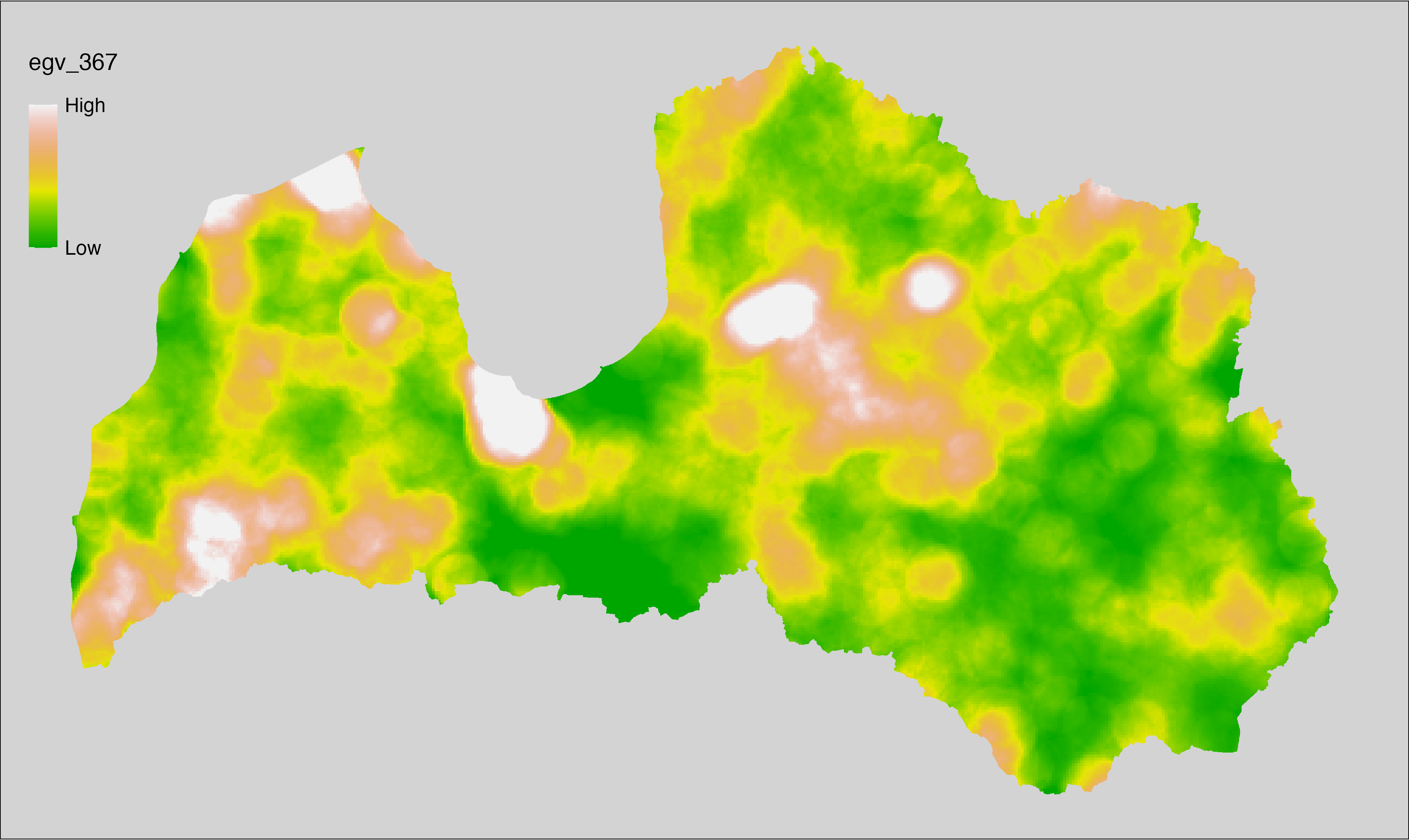
6.368 ForestsTreesAge_MixedYoung_cell
filename: ForestsTreesAge_MixedYoung_cell.tif
layername: egv_368
English name: Fractional cover of Young (pre-rotation age) Mixed Forests within the analysis cell (1 ha)
Latvian name: Jaunu (pirms cirtmeta) jauktu koku mežu platības īpatsvars analīzes šūnā (1 ha)
Procedure: Most EGVs describing forests are spatially restricted to areas outside of clearcuts and dead stands. This mask is created using a combination of the State Forest Service’s State Forest Registry land category 12 and 14, and The Global Forest Watch pixels classified as lost tree canopy cover since 2020 (raster layer matching input, presence = 1, absence = 0).
To prepare this EGV, stands from the State Forest Service’s State Forest Registry are classified into (in order):
coniferous (see Terminology and acronyms for species codes) if timber volume of those species exceeded 75%;
Boreal deciduous if timber volume of those species exceeded 75%;
temperate deciduous if timber volume of those species exceeded 50%;
mixed otherwise;
then mixed stands younger than the legal rotation age are selected and
geometries are rasterised (presence = 1, NA otherwise). Rasterisation is
performed using the workflow egvtools::polygon2input(), restricting to pixels outside clearcut
mask and covering background with value 0. The resulting layer
is then aggregated to EGV resolution using the workflow egvtools::input2egv(), which
calculates the arithmetic mean to determine the cover fraction. During
aggregation, inverse distance weighted (power = 2) gap filling on the output is
applied to ensure no missing values at the edges. Finally, the layer is
standardised by subtracting the arithmetic mean and dividing by the root mean squared
error.
Code
# libs ----
if(!require(egvtools)) {remotes::install_github("aavotins/egvtools"); require(egvtools)}
if(!require(terra)) {install.packages("terra"); require(terra)}
if(!require(sf)) {install.packages("sf"); require(sf)}
if(!require(tidyverse)) {install.packages("tidyverse"); require(tidyverse)}
if(!require(sfarrow)) {install.packages("sfarrow"); require(sfarrow)}
if(!require(readxl)) {install.packages("readxl"); require(readxl)}
if(!require(raster)) {install.packages("raster"); require(raster)}
if(!require(fasterize)) {install.packages("fasterize"); require(fasterize)}
# templates ----
template100=rast("./Templates/TemplateRasters/LV100m_10km.tif")
template10=rast("./Templates/TemplateRasters/LV10m_10km.tif")
rastrs10=raster(template10)
nulls10=rast("./Templates/TemplateRasters/nulls_LV10m_10km.tif")
nulls100=rast("./Templates/TemplateRasters/nulls_LV100m_10km.tif")
# simple landscape ----
simple_landscape=rast("RasterGrids_10m/2024/Ainava_vienk_mask.tif")
# mvr ----
mvr=st_read_parquet("./Geodata/2024/MVR/nogabali_2024janv.parquet")
mvr$yes=1
# clear cut mask ----
izcirtumi=mvr %>%
filter(zkat %in% c("12","14")) %>%
dplyr::select(yes)
r_izcirtumi_mvr=fasterize(izcirtumi,rastrs10,field="yes")
t_izcirtumi_mvr=rast(r_izcirtumi_mvr)
plot(t_izcirtumi_mvr)
tcl=rast("./Geodata/2024/Trees/GFW/TreeCoverLoss_v1_12.tif")
tcl2=ifel(tcl<20,0,1)
tclX=cover(tcl2,nulls10)
plot(tclX)
clearcut_mask=cover(t_izcirtumi_mvr,tclX,
filename="./RasterGrids_10m/2024/Mask_clearcuts.tif",
overwrite=TRUE)
plot(clearcut_mask)
rm(izcirtumi)
rm(r_izcirtumi_mvr)
rm(t_izcirtumi_mvr)
rm(tcl)
rm(tcl2)
rm(tclX)
# ForestsTreesAge_MixedYoung_cell.tif egv_368 ----
skujkoki=c("1","3","13","14","15","22","23","28") # 8
saurlapji=c("4","6","8","9","19","20","21","32","35","68") # 10
platlapji=c("10","11","12","16","17","18","24","25","26","27","28","29","50",
"61","62","63","64","65","66","67","69") # 21
mvr=mvr %>%
mutate(kraja_skujkoku=ifelse(s10 %in% skujkoki,v10,0)+
ifelse(s11 %in% skujkoki,v11,0)+ifelse(s12 %in% skujkoki,v12,0)+
ifelse(s13 %in% skujkoki,v13,0)+ifelse(s14 %in% skujkoki,v14,0),
kraja_saurlapju=ifelse(s10 %in% saurlapji,v10,0)+
ifelse(s11 %in% saurlapji,v11,0)+ifelse(s12 %in% saurlapji,v12,0)+
ifelse(s13 %in% saurlapji,v13,0)+ifelse(s14 %in% saurlapji,v14,0),
kraja_platlapju=ifelse(s10 %in% platlapji,v10,0)+
ifelse(s11 %in% platlapji,v11,0)+ifelse(s12 %in% platlapji,v12,0)+
ifelse(s13 %in% platlapji,v13,0)+ifelse(s14 %in% platlapji,v14,0)) %>%
mutate(kopeja_kraja=kraja_skujkoku+kraja_platlapju+kraja_saurlapju) %>%
mutate(tips=ifelse(kraja_skujkoku/kopeja_kraja>=0.75,"skujkoku",
ifelse(kraja_saurlapju/kopeja_kraja>=0.75,"saurlapju",
ifelse(kraja_platlapju/kopeja_kraja>0.5,"platlapju",
"jauktu koku"))))
nogabali=mvr %>%
filter(zkat=="10"&tips=="jauktu koku"&(vgr=="1"|vgr=="2"|vgr=="3"))
p2i_rez=egvtools::polygon2input(vector_data = nogabali,
template_path = "./Templates/TemplateRasters/LV10m_10km.tif",
out_path = "./RasterGrids_10m/2024/",
file_name = "ForestsTreesAge_MixedYoung_input.tif",
value_field = "yes",
restrict_to = clearcut_mask,
restrict_values = 0,
prepare=FALSE,
background_raster = "./Templates/TemplateRasters/nulls_LV10m_10km.tif",
plot_result = TRUE)
p2i_rez
i2e_rez=egvtools::input2egv(input=paste0("./RasterGrids_10m/2024/",
"ForestsTreesAge_MixedYoung_input.tif"),
egv_template= "./Templates/TemplateRasters/LV100m_10km.tif",
summary_function = "average",
missing_job = "FillOutput",
outlocation = "./RasterGrids_100m/2024/RAW/",
outfilename = "ForestsTreesAge_MixedYoung_cell.tif",
layername = "egv_368",
idw_weight = 2,
plot_gaps = FALSE,plot_final = TRUE)
i2e_rez
rm(nogabali)
rm(p2i_rez)
rm(i2e_rez)
unlink("./RasterGrids_10m/2024/ForestsTreesAge_MixedYoung_input.tif")
# standardisation ----
if(!require(terra)) {install.packages("terra"); require(terra)}
if(!require(tidyverse)) {install.packages("tidyverse"); require(tidyverse)}
nosaukums="ForestsTreesAge_MixedYoung_cell.tif"
ielasisanas_cels=paste0("./RasterGrids_100m/2024/RAW/",nosaukums)
saglabasanas_cels=paste0("./RasterGrids_100m/2024/Scaled/",nosaukums)
slanis=rast(ielasisanas_cels)
videjais=global(slanis,fun="mean",na.rm=TRUE)
centrets=slanis-videjais[,1]
standartnovirze=terra::global(centrets,fun="rms",na.rm=TRUE)
merogots=centrets/standartnovirze[,1]
writeRaster(merogots,
filename=saglabasanas_cels,
overwrite=TRUE)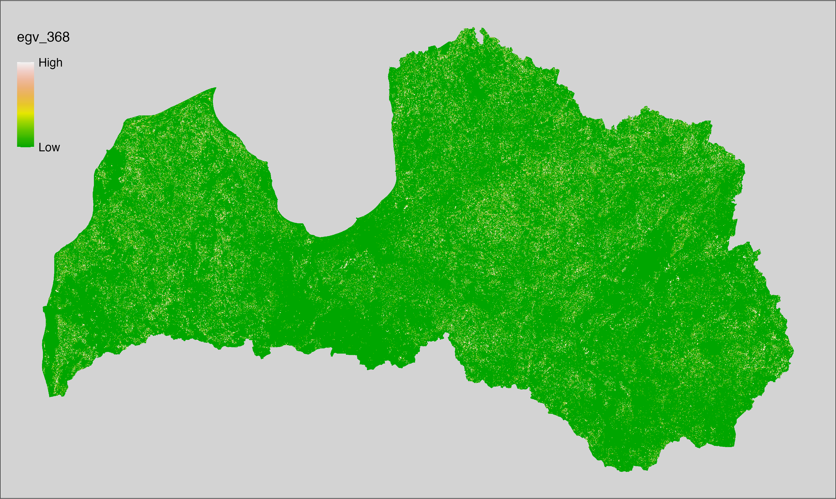
6.369 ForestsTreesAge_MixedYoung_r500
filename: ForestsTreesAge_MixedYoung_r500.tif
layername: egv_369
English name: Fractional cover of Young (pre-rotation age) Mixed Forests within the 0.5 km landscape
Latvian name: Jaunu (pirms cirtmeta) jauktu koku mežu platības īpatsvars 0,5 km ainavā
Procedure: The cover fraction within a radius of 500 m around the analysis grid cell is
calculated as the area-weighted sum of the analysis cells inside the
buffer, using the workflow egvtools::radius_function(). During the calculation of the landscape metric,
inverse distance weighted (power = 2) gap filling on the output is applied
to ensure no missing values at the edges. Then the layer is rewritten to set
its name. Finally, the layer is standardised by subtracting the arithmetic
mean and dividing by the root mean squared error.
Code
# libs ----
if(!require(terra)) {install.packages("terra"); require(terra)}
if(!require(egvtools)) {remotes::install_github("aavotins/egvtools"); require(egvtools)}
# Templates -----
template100=rast("./Templates/TemplateRasters/LV100m_10km.tif")
# radii ----
radius_function(
kvadrati_path = "./Templates/TemplateGrids/tiles/",
radii_path = "./Templates/TemplateGridPoints/tiles/",
tikls100_path = "./Templates/TemplateGrids/tikls100_sauzeme.parquet",
template_path = "./Templates/TemplateRasters/LV100m_10km.tif",
input_layers = c("./RasterGrids_100m/2024/RAW/ForestsTreesAge_MixedYoung_cell.tif"),
layer_prefixes = c("ForestsTreesAge_MixedYoung"),
output_dir = "./RasterGrids_100m/2024/RAW/",
n_workers = 6,
radii = c("r500"),
radius_mode = "sparse",
extract_fun = "mean",
fill_missing = TRUE,
IDW_weight = 2,
future_max_size = 40 * 1024^3)
# ForestsTreesAge_MixedYoung_r500.tif egv_369
slanis=rast("./RasterGrids_100m/2024/RAW/ForestsTreesAge_MixedYoung_r500.tif")
names(slanis)="egv_369"
slanis2=project(slanis,template100)
writeRaster(slanis2,
"./RasterGrids_100m/2024/RAW/ForestsTreesAge_MixedYoung_r500.tif",
overwrite=TRUE)
# standardisation ----
if(!require(terra)) {install.packages("terra"); require(terra)}
if(!require(tidyverse)) {install.packages("tidyverse"); require(tidyverse)}
nosaukums="ForestsTreesAge_MixedYoung_r500.tif"
ielasisanas_cels=paste0("./RasterGrids_100m/2024/RAW/",nosaukums)
saglabasanas_cels=paste0("./RasterGrids_100m/2024/Scaled/",nosaukums)
slanis=rast(ielasisanas_cels)
videjais=global(slanis,fun="mean",na.rm=TRUE)
centrets=slanis-videjais[,1]
standartnovirze=terra::global(centrets,fun="rms",na.rm=TRUE)
merogots=centrets/standartnovirze[,1]
writeRaster(merogots,
filename=saglabasanas_cels,
overwrite=TRUE)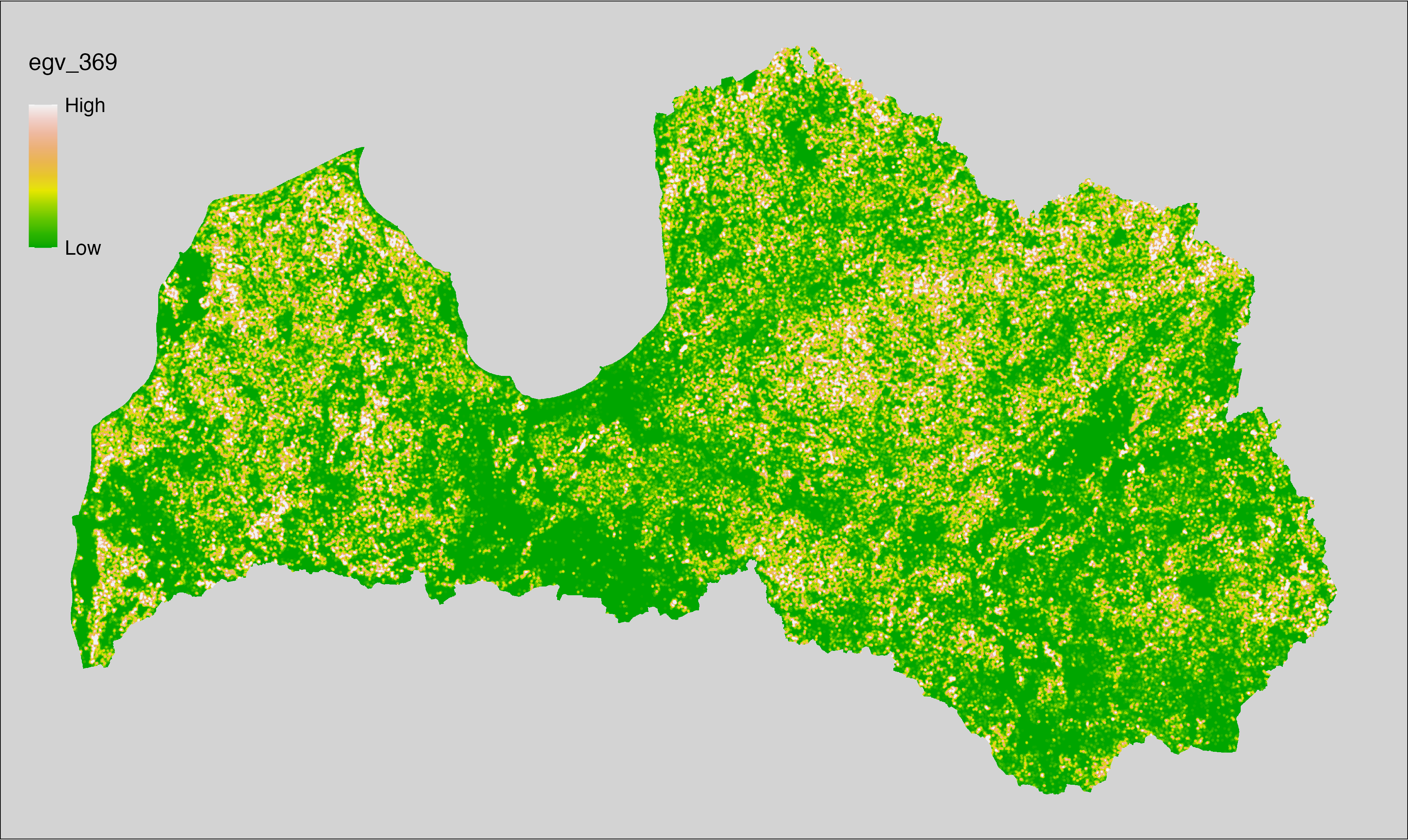
6.370 ForestsTreesAge_MixedYoung_r1250
filename: ForestsTreesAge_MixedYoung_r1250.tif
layername: egv_370
English name: Fractional cover of Young (pre-rotation age) Mixed Forests within the 1.25 km landscape
Latvian name: Jaunu (pirms cirtmeta) jauktu koku mežu platības īpatsvars 1,25 km ainavā
Procedure: The cover fraction within a radius of 1250 m around the analysis grid cell
is calculated as the area-weighted sum of the analysis cells inside
the buffer, using the workflow egvtools::radius_function(). During the calculation of the landscape
metric, inverse distance weighted (power = 2) gap filling on the output is
applied to ensure no missing values at the edges. Then the layer is
rewritten to set its name. Finally, the layer is standardised by
subtracting the arithmetic mean and dividing by the root mean squared error.
Code
# libs ----
if(!require(terra)) {install.packages("terra"); require(terra)}
if(!require(egvtools)) {remotes::install_github("aavotins/egvtools"); require(egvtools)}
# Templates -----
template100=rast("./Templates/TemplateRasters/LV100m_10km.tif")
# radii ----
radius_function(
kvadrati_path = "./Templates/TemplateGrids/tiles/",
radii_path = "./Templates/TemplateGridPoints/tiles/",
tikls100_path = "./Templates/TemplateGrids/tikls100_sauzeme.parquet",
template_path = "./Templates/TemplateRasters/LV100m_10km.tif",
input_layers = c("./RasterGrids_100m/2024/RAW/ForestsTreesAge_MixedYoung_cell.tif"),
layer_prefixes = c("ForestsTreesAge_MixedYoung"),
output_dir = "./RasterGrids_100m/2024/RAW/",
n_workers = 6,
radii = c("r1250"),
radius_mode = "sparse",
extract_fun = "mean",
fill_missing = TRUE,
IDW_weight = 2,
future_max_size = 40 * 1024^3)
# ForestsTreesAge_MixedYoung_r1250.tif egv_370
slanis=rast("./RasterGrids_100m/2024/RAW/ForestsTreesAge_MixedYoung_r1250.tif")
names(slanis)="egv_370"
slanis2=project(slanis,template100)
writeRaster(slanis2,
"./RasterGrids_100m/2024/RAW/ForestsTreesAge_MixedYoung_r1250.tif",
overwrite=TRUE)
# standardisation ----
if(!require(terra)) {install.packages("terra"); require(terra)}
if(!require(tidyverse)) {install.packages("tidyverse"); require(tidyverse)}
nosaukums="ForestsTreesAge_MixedYoung_r1250.tif"
ielasisanas_cels=paste0("./RasterGrids_100m/2024/RAW/",nosaukums)
saglabasanas_cels=paste0("./RasterGrids_100m/2024/Scaled/",nosaukums)
slanis=rast(ielasisanas_cels)
videjais=global(slanis,fun="mean",na.rm=TRUE)
centrets=slanis-videjais[,1]
standartnovirze=terra::global(centrets,fun="rms",na.rm=TRUE)
merogots=centrets/standartnovirze[,1]
writeRaster(merogots,
filename=saglabasanas_cels,
overwrite=TRUE)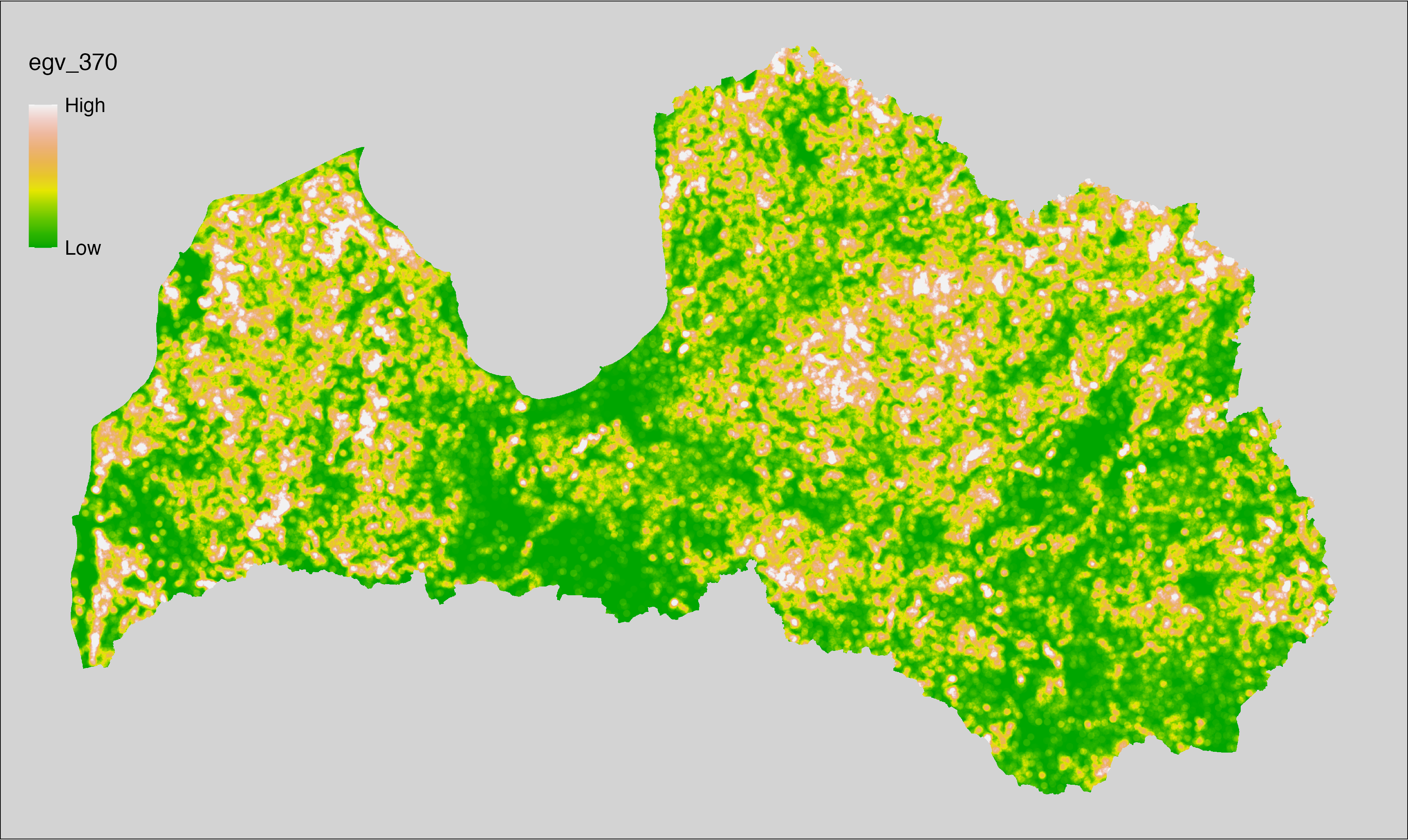
6.371 ForestsTreesAge_MixedYoung_r3000
filename: ForestsTreesAge_MixedYoung_r3000.tif
layername: egv_371
English name: Fractional cover of Young (pre-rotation age) Mixed Forests within the 3 km landscape
Latvian name: Jaunu (pirms cirtmeta) jauktu koku mežu platības īpatsvars 3 km ainavā
Procedure: The cover fraction within a radius of 3000 m around the analysis grid cell
is calculated as the area-weighted sum of the analysis cells inside
the buffer, using the workflow egvtools::radius_function(). During the calculation of the landscape
metric, inverse distance weighted (power = 2) gap filling on the output is
applied to ensure no missing values at the edges. Then the layer is
rewritten to set its name. Finally, the layer is standardised by
subtracting the arithmetic mean and dividing by the root mean squared error.
Code
# libs ----
if(!require(terra)) {install.packages("terra"); require(terra)}
if(!require(egvtools)) {remotes::install_github("aavotins/egvtools"); require(egvtools)}
# Templates -----
template100=rast("./Templates/TemplateRasters/LV100m_10km.tif")
# radii ----
radius_function(
kvadrati_path = "./Templates/TemplateGrids/tiles/",
radii_path = "./Templates/TemplateGridPoints/tiles/",
tikls100_path = "./Templates/TemplateGrids/tikls100_sauzeme.parquet",
template_path = "./Templates/TemplateRasters/LV100m_10km.tif",
input_layers = c("./RasterGrids_100m/2024/RAW/ForestsTreesAge_MixedYoung_cell.tif"),
layer_prefixes = c("ForestsTreesAge_MixedYoung"),
output_dir = "./RasterGrids_100m/2024/RAW/",
n_workers = 6,
radii = c("r3000"),
radius_mode = "sparse",
extract_fun = "mean",
fill_missing = TRUE,
IDW_weight = 2,
future_max_size = 40 * 1024^3)
# ForestsTreesAge_MixedYoung_r3000.tif egv_371
slanis=rast("./RasterGrids_100m/2024/RAW/ForestsTreesAge_MixedYoung_r3000.tif")
names(slanis)="egv_371"
slanis2=project(slanis,template100)
writeRaster(slanis2,
"./RasterGrids_100m/2024/RAW/ForestsTreesAge_MixedYoung_r3000.tif",
overwrite=TRUE)
# standardisation ----
if(!require(terra)) {install.packages("terra"); require(terra)}
if(!require(tidyverse)) {install.packages("tidyverse"); require(tidyverse)}
nosaukums="ForestsTreesAge_MixedYoung_r3000.tif"
ielasisanas_cels=paste0("./RasterGrids_100m/2024/RAW/",nosaukums)
saglabasanas_cels=paste0("./RasterGrids_100m/2024/Scaled/",nosaukums)
slanis=rast(ielasisanas_cels)
videjais=global(slanis,fun="mean",na.rm=TRUE)
centrets=slanis-videjais[,1]
standartnovirze=terra::global(centrets,fun="rms",na.rm=TRUE)
merogots=centrets/standartnovirze[,1]
writeRaster(merogots,
filename=saglabasanas_cels,
overwrite=TRUE)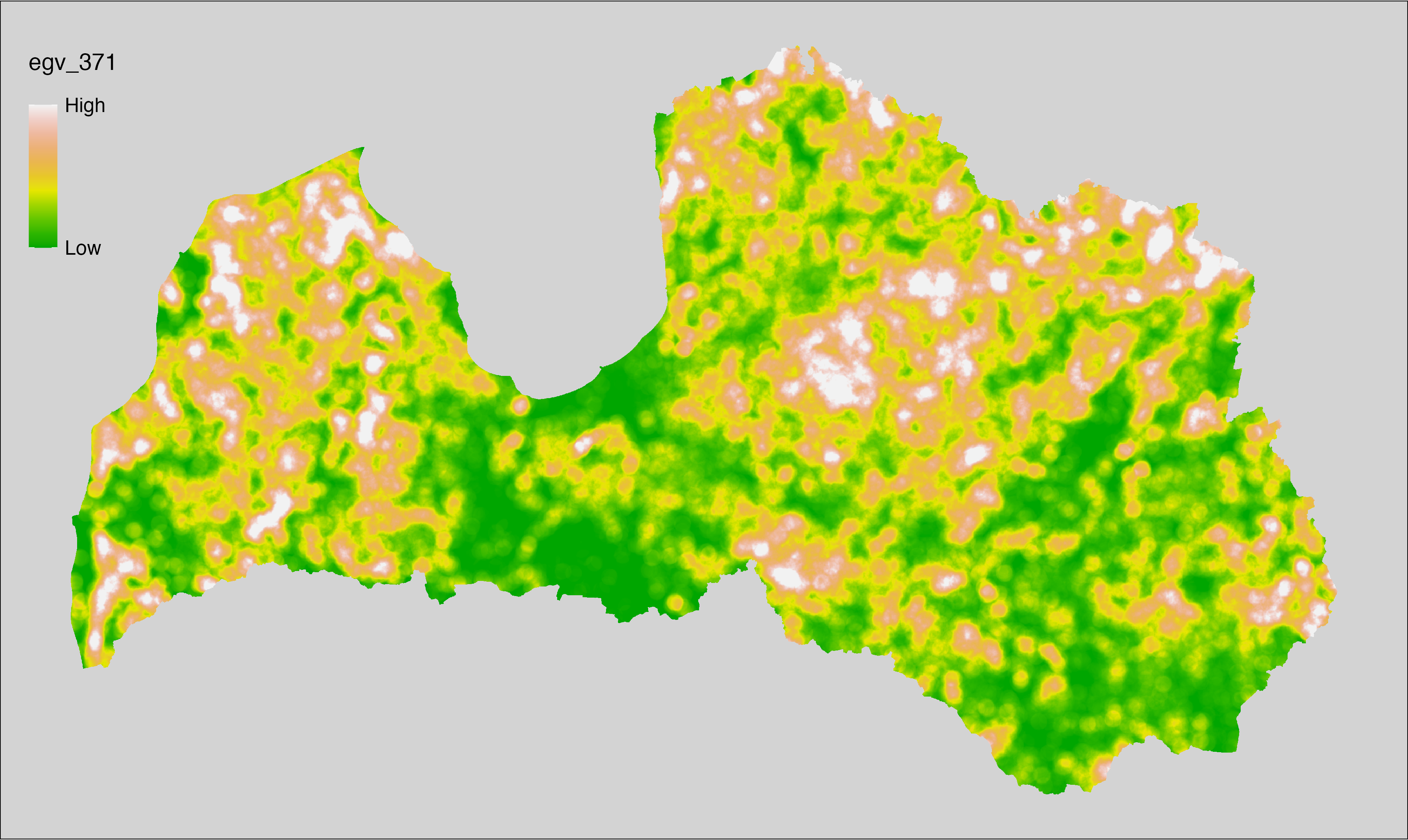
6.372 ForestsTreesAge_MixedYoung_r10000
filename: ForestsTreesAge_MixedYoung_r10000.tif
layername: egv_372
English name: Fractional cover of Young (pre-rotation age) Mixed Forests within the 10 km landscape
Latvian name: Jaunu (pirms cirtmeta) jauktu koku mežu platības īpatsvars 10 km ainavā
Procedure: The cover fraction within a radius of 10000 m around the analysis grid cell
is calculated as the area-weighted sum of the analysis cells inside
the buffer, using the workflow egvtools::radius_function(). During the calculation of the landscape
metric, inverse distance weighted (power = 2) gap filling on the output is
applied to ensure no missing values at the edges. Then the layer is
rewritten to set its name. Finally, the layer is standardised by
subtracting the arithmetic mean and dividing by the root mean squared error.
Code
# libs ----
if(!require(terra)) {install.packages("terra"); require(terra)}
if(!require(egvtools)) {remotes::install_github("aavotins/egvtools"); require(egvtools)}
# Templates -----
template100=rast("./Templates/TemplateRasters/LV100m_10km.tif")
# radii ----
radius_function(
kvadrati_path = "./Templates/TemplateGrids/tiles/",
radii_path = "./Templates/TemplateGridPoints/tiles/",
tikls100_path = "./Templates/TemplateGrids/tikls100_sauzeme.parquet",
template_path = "./Templates/TemplateRasters/LV100m_10km.tif",
input_layers = c("./RasterGrids_100m/2024/RAW/ForestsTreesAge_MixedYoung_cell.tif"),
layer_prefixes = c("ForestsTreesAge_MixedYoung"),
output_dir = "./RasterGrids_100m/2024/RAW/",
n_workers = 6,
radii = c("r10000"),
radius_mode = "sparse",
extract_fun = "mean",
fill_missing = TRUE,
IDW_weight = 2,
future_max_size = 40 * 1024^3)
# ForestsTreesAge_MixedYoung_r10000.tif egv_372
slanis=rast("./RasterGrids_100m/2024/RAW/ForestsTreesAge_MixedYoung_r10000.tif")
names(slanis)="egv_372"
slanis2=project(slanis,template100)
writeRaster(slanis2,
"./RasterGrids_100m/2024/RAW/ForestsTreesAge_MixedYoung_r10000.tif",
overwrite=TRUE)
# standardisation ----
if(!require(terra)) {install.packages("terra"); require(terra)}
if(!require(tidyverse)) {install.packages("tidyverse"); require(tidyverse)}
nosaukums="ForestsTreesAge_MixedYoung_r10000.tif"
ielasisanas_cels=paste0("./RasterGrids_100m/2024/RAW/",nosaukums)
saglabasanas_cels=paste0("./RasterGrids_100m/2024/Scaled/",nosaukums)
slanis=rast(ielasisanas_cels)
videjais=global(slanis,fun="mean",na.rm=TRUE)
centrets=slanis-videjais[,1]
standartnovirze=terra::global(centrets,fun="rms",na.rm=TRUE)
merogots=centrets/standartnovirze[,1]
writeRaster(merogots,
filename=saglabasanas_cels,
overwrite=TRUE)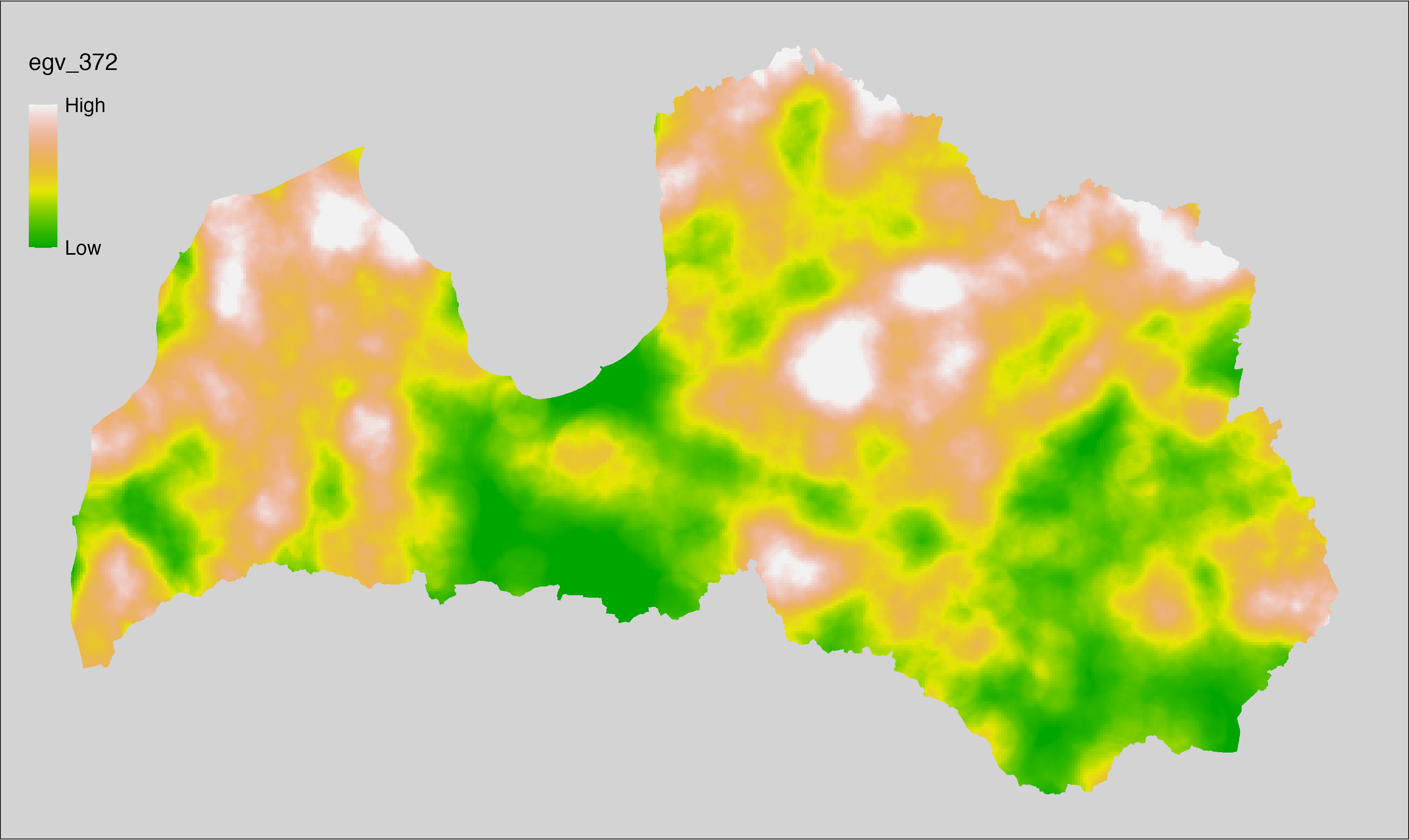
6.373 ForestsTreesAge_TemperateDeciduousOld_cell
filename: ForestsTreesAge_TemperateDeciduousOld_cell.tif
layername: egv_373
English name: Fractional cover of Old (over rotation age) Temperate Deciduous Forests within the analysis cell (1 ha)
Latvian name: Vecu (kopš cirtmeta) platlapju mežu platības īpatsvars analīzes šūnā (1 ha)
Procedure: Most EGVs describing forests are spatially restricted to areas outside of clearcuts and dead stands. This mask is created using a combination of the State Forest Service’s State Forest Registry land category 12 and 14, and The Global Forest Watch pixels classified as lost tree canopy cover since 2020 (raster layer matching input, presence = 1, absence = 0).
To prepare this EGV, stands from the State Forest Service’s State Forest Registry are classified into (in order):
coniferous (see Terminology and acronyms for species codes) if timber volume of those species exceeded 75%;
Boreal deciduous if timber volume of those species exceeded 75%;
temperate deciduous if timber volume of those species exceeded 50%;
mixed otherwise;
then temperate deciduous stands exceeding the legal rotation age are selected
and geometries are rasterised (presence = 1, NA otherwise). Rasterisation is
performed using the workflow egvtools::polygon2input(), restricting to pixels outside clearcut
mask and covering background with value 0. The resulting layer
is then aggregated to EGV resolution using the workflow egvtools::input2egv(), which
calculates the arithmetic mean to determine the cover fraction. During
aggregation, inverse distance weighted (power = 2) gap filling on the output is
applied to ensure no missing values at the edges. Finally, the layer is
standardised by subtracting the arithmetic mean and dividing by the root mean squared
error.
Code
# libs ----
if(!require(egvtools)) {remotes::install_github("aavotins/egvtools"); require(egvtools)}
if(!require(terra)) {install.packages("terra"); require(terra)}
if(!require(sf)) {install.packages("sf"); require(sf)}
if(!require(tidyverse)) {install.packages("tidyverse"); require(tidyverse)}
if(!require(sfarrow)) {install.packages("sfarrow"); require(sfarrow)}
if(!require(readxl)) {install.packages("readxl"); require(readxl)}
if(!require(raster)) {install.packages("raster"); require(raster)}
if(!require(fasterize)) {install.packages("fasterize"); require(fasterize)}
# templates ----
template100=rast("./Templates/TemplateRasters/LV100m_10km.tif")
template10=rast("./Templates/TemplateRasters/LV10m_10km.tif")
rastrs10=raster(template10)
nulls10=rast("./Templates/TemplateRasters/nulls_LV10m_10km.tif")
nulls100=rast("./Templates/TemplateRasters/nulls_LV100m_10km.tif")
# simple landscape ----
simple_landscape=rast("RasterGrids_10m/2024/Ainava_vienk_mask.tif")
# mvr ----
mvr=st_read_parquet("./Geodata/2024/MVR/nogabali_2024janv.parquet")
mvr$yes=1
# clear cut mask ----
izcirtumi=mvr %>%
filter(zkat %in% c("12","14")) %>%
dplyr::select(yes)
r_izcirtumi_mvr=fasterize(izcirtumi,rastrs10,field="yes")
t_izcirtumi_mvr=rast(r_izcirtumi_mvr)
plot(t_izcirtumi_mvr)
tcl=rast("./Geodata/2024/Trees/GFW/TreeCoverLoss_v1_12.tif")
tcl2=ifel(tcl<20,0,1)
tclX=cover(tcl2,nulls10)
plot(tclX)
clearcut_mask=cover(t_izcirtumi_mvr,tclX,
filename="./RasterGrids_10m/2024/Mask_clearcuts.tif",
overwrite=TRUE)
plot(clearcut_mask)
rm(izcirtumi)
rm(r_izcirtumi_mvr)
rm(t_izcirtumi_mvr)
rm(tcl)
rm(tcl2)
rm(tclX)
# ForestsTreesAge_TemperateDeciduousOld_cell.tif egv_373 ----
skujkoki=c("1","3","13","14","15","22","23","28") # 8
saurlapji=c("4","6","8","9","19","20","21","32","35","68") # 10
platlapji=c("10","11","12","16","17","18","24","25","26","27","28","29","50",
"61","62","63","64","65","66","67","69") # 21
mvr=mvr %>%
mutate(kraja_skujkoku=ifelse(s10 %in% skujkoki,v10,0)+
ifelse(s11 %in% skujkoki,v11,0)+ifelse(s12 %in% skujkoki,v12,0)+
ifelse(s13 %in% skujkoki,v13,0)+ifelse(s14 %in% skujkoki,v14,0),
kraja_saurlapju=ifelse(s10 %in% saurlapji,v10,0)+
ifelse(s11 %in% saurlapji,v11,0)+ifelse(s12 %in% saurlapji,v12,0)+
ifelse(s13 %in% saurlapji,v13,0)+ifelse(s14 %in% saurlapji,v14,0),
kraja_platlapju=ifelse(s10 %in% platlapji,v10,0)+
ifelse(s11 %in% platlapji,v11,0)+ifelse(s12 %in% platlapji,v12,0)+
ifelse(s13 %in% platlapji,v13,0)+ifelse(s14 %in% platlapji,v14,0)) %>%
mutate(kopeja_kraja=kraja_skujkoku+kraja_platlapju+kraja_saurlapju) %>%
mutate(tips=ifelse(kraja_skujkoku/kopeja_kraja>=0.75,"skujkoku",
ifelse(kraja_saurlapju/kopeja_kraja>=0.75,"saurlapju",
ifelse(kraja_platlapju/kopeja_kraja>0.5,"platlapju",
"jauktu koku"))))
nogabali=mvr %>%
filter(zkat=="10"&tips=="platlapju"&(vgr=="4"|vgr=="5"))
p2i_rez=egvtools::polygon2input(vector_data = nogabali,
template_path = "./Templates/TemplateRasters/LV10m_10km.tif",
out_path = "./RasterGrids_10m/2024/",
file_name = "ForestsTreesAge_TemperateDeciduousOld_input.tif",
value_field = "yes",
restrict_to = clearcut_mask,
restrict_values = 0,
prepare=FALSE,
background_raster = "./Templates/TemplateRasters/nulls_LV10m_10km.tif",
plot_result = TRUE)
p2i_rez
i2e_rez=egvtools::input2egv(input=paste0("./RasterGrids_10m/2024/",
"ForestsTreesAge_TemperateDeciduousOld_input.tif"),
egv_template= "./Templates/TemplateRasters/LV100m_10km.tif",
summary_function = "average",
missing_job = "FillOutput",
outlocation = "./RasterGrids_100m/2024/RAW/",
outfilename = "ForestsTreesAge_TemperateDeciduousOld_cell.tif",
layername = "egv_373",
idw_weight = 2,
plot_gaps = FALSE,plot_final = TRUE)
i2e_rez
rm(nogabali)
rm(p2i_rez)
rm(i2e_rez)
unlink("./RasterGrids_10m/2024/ForestsTreesAge_TemperateDeciduousOld_input.tif")
# standardisation ----
if(!require(terra)) {install.packages("terra"); require(terra)}
if(!require(tidyverse)) {install.packages("tidyverse"); require(tidyverse)}
nosaukums="ForestsTreesAge_TemperateDeciduousOld_cell.tif"
ielasisanas_cels=paste0("./RasterGrids_100m/2024/RAW/",nosaukums)
saglabasanas_cels=paste0("./RasterGrids_100m/2024/Scaled/",nosaukums)
slanis=rast(ielasisanas_cels)
videjais=global(slanis,fun="mean",na.rm=TRUE)
centrets=slanis-videjais[,1]
standartnovirze=terra::global(centrets,fun="rms",na.rm=TRUE)
merogots=centrets/standartnovirze[,1]
writeRaster(merogots,
filename=saglabasanas_cels,
overwrite=TRUE)
6.374 ForestsTreesAge_TemperateDeciduousOld_r500
filename: ForestsTreesAge_TemperateDeciduousOld_r500.tif
layername: egv_374
English name: Fractional cover of Old (over rotation age) Temperate Deciduous Forests within the 0.5 km landscape
Latvian name: Vecu (kopš cirtmeta) platlapju mežu platības īpatsvars 0,5 km ainavā
Procedure: The cover fraction within a radius of 500 m around the analysis grid cell is
calculated as the area-weighted sum of the analysis cells inside the
buffer, using the workflow egvtools::radius_function(). During the calculation of the landscape metric,
inverse distance weighted (power = 2) gap filling on the output is applied
to ensure no missing values at the edges. Then the layer is rewritten to set
its name. Finally, the layer is standardised by subtracting the arithmetic
mean and dividing by the root mean squared error.
Code
# libs ----
if(!require(terra)) {install.packages("terra"); require(terra)}
if(!require(egvtools)) {remotes::install_github("aavotins/egvtools"); require(egvtools)}
# Templates -----
template100=rast("./Templates/TemplateRasters/LV100m_10km.tif")
# radii ----
radius_function(
kvadrati_path = "./Templates/TemplateGrids/tiles/",
radii_path = "./Templates/TemplateGridPoints/tiles/",
tikls100_path = "./Templates/TemplateGrids/tikls100_sauzeme.parquet",
template_path = "./Templates/TemplateRasters/LV100m_10km.tif",
input_layers = c("./RasterGrids_100m/2024/RAW/ForestsTreesAge_TemperateDeciduousOld_cell.tif"),
layer_prefixes = c("ForestsTreesAge_TemperateDeciduousOld"),
output_dir = "./RasterGrids_100m/2024/RAW/",
n_workers = 6,
radii = c("r500"),
radius_mode = "sparse",
extract_fun = "mean",
fill_missing = TRUE,
IDW_weight = 2,
future_max_size = 40 * 1024^3)
# ForestsTreesAge_TemperateDeciduousOld_r500.tif egv_374
slanis=rast("./RasterGrids_100m/2024/RAW/ForestsTreesAge_TemperateDeciduousOld_r500.tif")
names(slanis)="egv_374"
slanis2=project(slanis,template100)
writeRaster(slanis2,
"./RasterGrids_100m/2024/RAW/ForestsTreesAge_TemperateDeciduousOld_r500.tif",
overwrite=TRUE)
# standardisation ----
if(!require(terra)) {install.packages("terra"); require(terra)}
if(!require(tidyverse)) {install.packages("tidyverse"); require(tidyverse)}
nosaukums="ForestsTreesAge_TemperateDeciduousOld_r500.tif"
ielasisanas_cels=paste0("./RasterGrids_100m/2024/RAW/",nosaukums)
saglabasanas_cels=paste0("./RasterGrids_100m/2024/Scaled/",nosaukums)
slanis=rast(ielasisanas_cels)
videjais=global(slanis,fun="mean",na.rm=TRUE)
centrets=slanis-videjais[,1]
standartnovirze=terra::global(centrets,fun="rms",na.rm=TRUE)
merogots=centrets/standartnovirze[,1]
writeRaster(merogots,
filename=saglabasanas_cels,
overwrite=TRUE)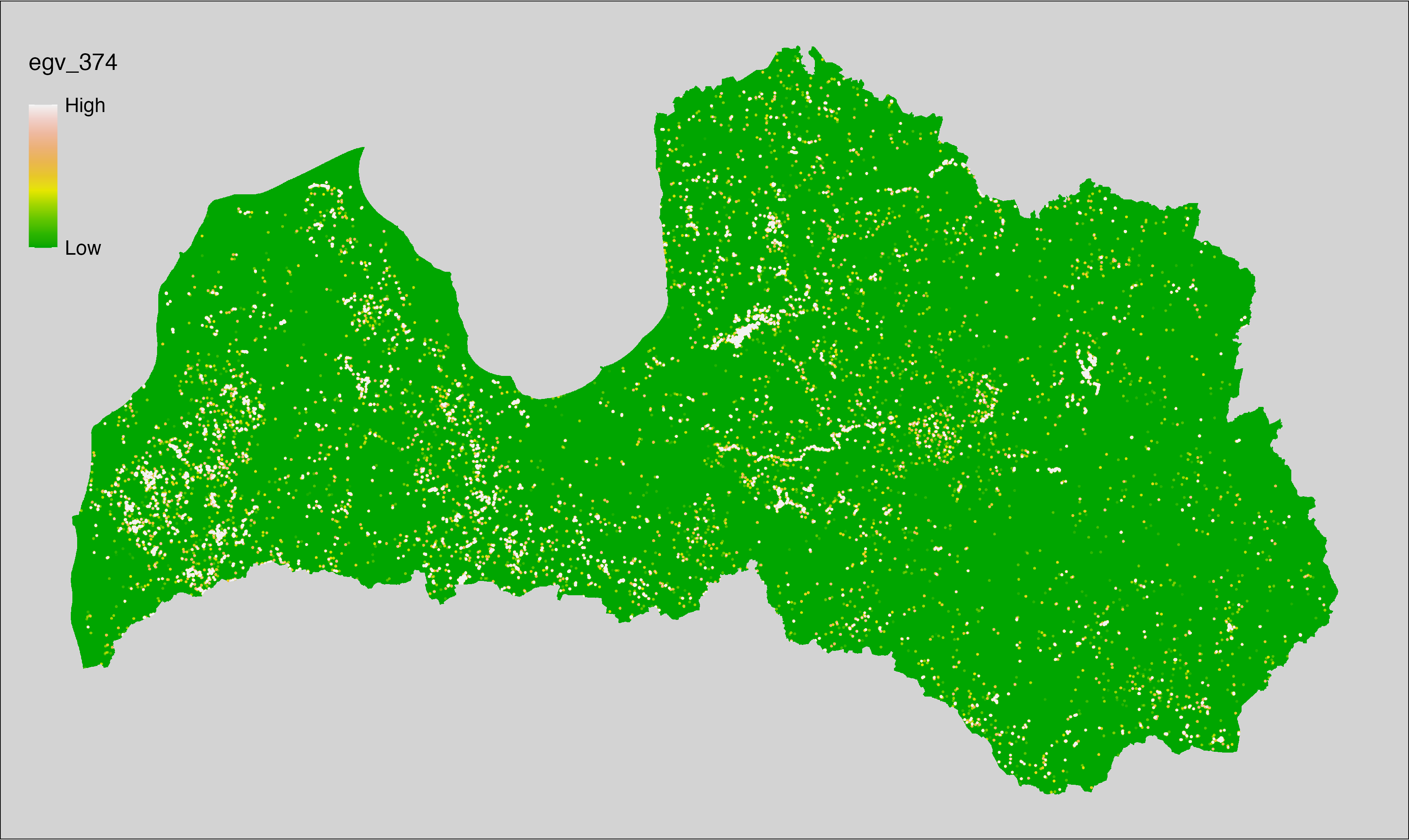
6.375 ForestsTreesAge_TemperateDeciduousOld_r1250
filename: ForestsTreesAge_TemperateDeciduousOld_r1250.tif
layername: egv_375
English name: Fractional cover of Old (over rotation age) Temperate Deciduous Forests within the 1.25 km landscape
Latvian name: Vecu (kopš cirtmeta) platlapju mežu platības īpatsvars 1,25 km ainavā
Procedure: The cover fraction within a radius of 1250 m around the analysis grid cell
is calculated as the area-weighted sum of the analysis cells inside
the buffer, using the workflow egvtools::radius_function(). During the calculation of the landscape
metric, inverse distance weighted (power = 2) gap filling on the output is
applied to ensure no missing values at the edges. Then the layer is
rewritten to set its name. Finally, the layer is standardised by
subtracting the arithmetic mean and dividing by the root mean squared error.
Code
# libs ----
if(!require(terra)) {install.packages("terra"); require(terra)}
if(!require(egvtools)) {remotes::install_github("aavotins/egvtools"); require(egvtools)}
# Templates -----
template100=rast("./Templates/TemplateRasters/LV100m_10km.tif")
# radii ----
radius_function(
kvadrati_path = "./Templates/TemplateGrids/tiles/",
radii_path = "./Templates/TemplateGridPoints/tiles/",
tikls100_path = "./Templates/TemplateGrids/tikls100_sauzeme.parquet",
template_path = "./Templates/TemplateRasters/LV100m_10km.tif",
input_layers = c("./RasterGrids_100m/2024/RAW/ForestsTreesAge_TemperateDeciduousOld_cell.tif"),
layer_prefixes = c("ForestsTreesAge_TemperateDeciduousOld"),
output_dir = "./RasterGrids_100m/2024/RAW/",
n_workers = 6,
radii = c("r1250"),
radius_mode = "sparse",
extract_fun = "mean",
fill_missing = TRUE,
IDW_weight = 2,
future_max_size = 40 * 1024^3)
# ForestsTreesAge_TemperateDeciduousOld_r1250.tif egv_375
slanis=rast("./RasterGrids_100m/2024/RAW/ForestsTreesAge_TemperateDeciduousOld_r1250.tif")
names(slanis)="egv_375"
slanis2=project(slanis,template100)
writeRaster(slanis2,
"./RasterGrids_100m/2024/RAW/ForestsTreesAge_TemperateDeciduousOld_r1250.tif",
overwrite=TRUE)
# standardisation ----
if(!require(terra)) {install.packages("terra"); require(terra)}
if(!require(tidyverse)) {install.packages("tidyverse"); require(tidyverse)}
nosaukums="ForestsTreesAge_TemperateDeciduousOld_r1250.tif"
ielasisanas_cels=paste0("./RasterGrids_100m/2024/RAW/",nosaukums)
saglabasanas_cels=paste0("./RasterGrids_100m/2024/Scaled/",nosaukums)
slanis=rast(ielasisanas_cels)
videjais=global(slanis,fun="mean",na.rm=TRUE)
centrets=slanis-videjais[,1]
standartnovirze=terra::global(centrets,fun="rms",na.rm=TRUE)
merogots=centrets/standartnovirze[,1]
writeRaster(merogots,
filename=saglabasanas_cels,
overwrite=TRUE)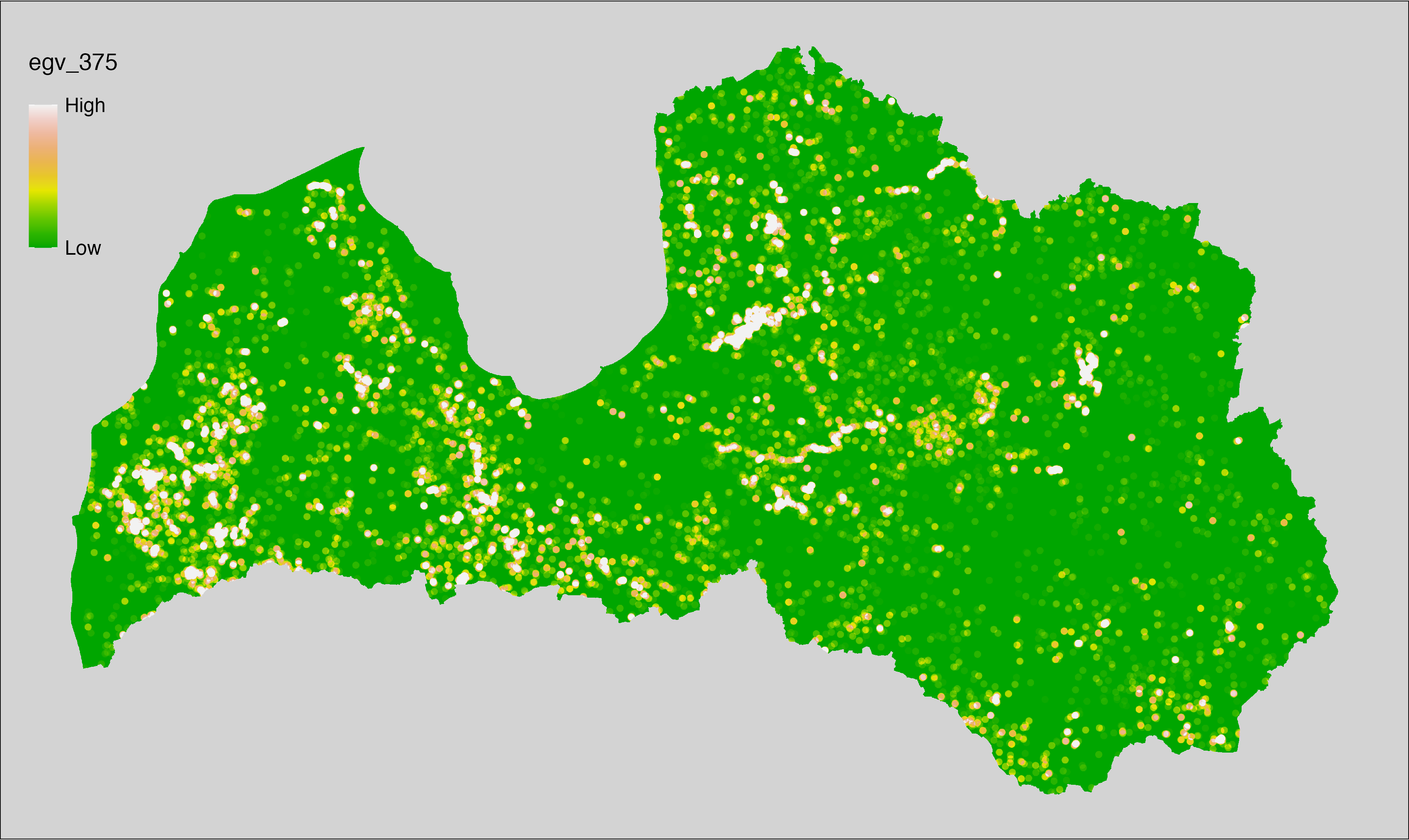
6.376 ForestsTreesAge_TemperateDeciduousOld_r3000
filename: ForestsTreesAge_TemperateDeciduousOld_r3000.tif
layername: egv_376
English name: Fractional cover of Old (over rotation age) Temperate Deciduous Forests within the 3 km landscape
Latvian name: Vecu (kopš cirtmeta) platlapju mežu platības īpatsvars 3 km ainavā
Procedure: The cover fraction within a radius of 3000 m around the analysis grid cell
is calculated as the area-weighted sum of the analysis cells inside
the buffer, using the workflow egvtools::radius_function(). During the calculation of the landscape
metric, inverse distance weighted (power = 2) gap filling on the output is
applied to ensure no missing values at the edges. Then the layer is
rewritten to set its name. Finally, the layer is standardised by
subtracting the arithmetic mean and dividing by the root mean squared error.
Code
# libs ----
if(!require(terra)) {install.packages("terra"); require(terra)}
if(!require(egvtools)) {remotes::install_github("aavotins/egvtools"); require(egvtools)}
# Templates -----
template100=rast("./Templates/TemplateRasters/LV100m_10km.tif")
# radii ----
radius_function(
kvadrati_path = "./Templates/TemplateGrids/tiles/",
radii_path = "./Templates/TemplateGridPoints/tiles/",
tikls100_path = "./Templates/TemplateGrids/tikls100_sauzeme.parquet",
template_path = "./Templates/TemplateRasters/LV100m_10km.tif",
input_layers = c("./RasterGrids_100m/2024/RAW/ForestsTreesAge_TemperateDeciduousOld_cell.tif"),
layer_prefixes = c("ForestsTreesAge_TemperateDeciduousOld"),
output_dir = "./RasterGrids_100m/2024/RAW/",
n_workers = 6,
radii = c("r3000"),
radius_mode = "sparse",
extract_fun = "mean",
fill_missing = TRUE,
IDW_weight = 2,
future_max_size = 40 * 1024^3)
# ForestsTreesAge_TemperateDeciduousOld_r3000.tif egv_376
slanis=rast("./RasterGrids_100m/2024/RAW/ForestsTreesAge_TemperateDeciduousOld_r3000.tif")
names(slanis)="egv_376"
slanis2=project(slanis,template100)
writeRaster(slanis2,
"./RasterGrids_100m/2024/RAW/ForestsTreesAge_TemperateDeciduousOld_r3000.tif",
overwrite=TRUE)
# standardisation ----
if(!require(terra)) {install.packages("terra"); require(terra)}
if(!require(tidyverse)) {install.packages("tidyverse"); require(tidyverse)}
nosaukums="ForestsTreesAge_TemperateDeciduousOld_r3000.tif"
ielasisanas_cels=paste0("./RasterGrids_100m/2024/RAW/",nosaukums)
saglabasanas_cels=paste0("./RasterGrids_100m/2024/Scaled/",nosaukums)
slanis=rast(ielasisanas_cels)
videjais=global(slanis,fun="mean",na.rm=TRUE)
centrets=slanis-videjais[,1]
standartnovirze=terra::global(centrets,fun="rms",na.rm=TRUE)
merogots=centrets/standartnovirze[,1]
writeRaster(merogots,
filename=saglabasanas_cels,
overwrite=TRUE)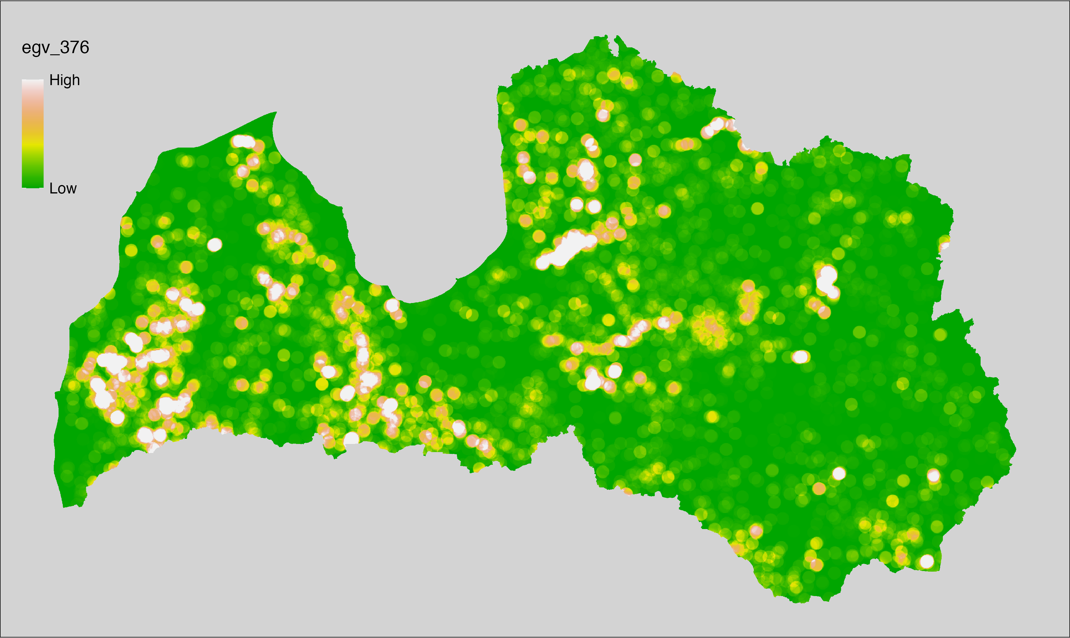
6.377 ForestsTreesAge_TemperateDeciduousOld_r10000
filename: ForestsTreesAge_TemperateDeciduousOld_r10000.tif
layername: egv_377
English name: Fractional cover of Old (over rotation age) Temperate Deciduous Forests within the 10 km landscape
Latvian name: Vecu (kopš cirtmeta) platlapju mežu platības īpatsvars 10 km ainavā
Procedure: The cover fraction within a radius of 10000 m around the analysis grid cell
is calculated as the area-weighted sum of the analysis cells inside
the buffer, using the workflow egvtools::radius_function(). During the calculation of the landscape
metric, inverse distance weighted (power = 2) gap filling on the output is
applied to ensure no missing values at the edges. Then the layer is
rewritten to set its name. Finally, the layer is standardised by
subtracting the arithmetic mean and dividing by the root mean squared error.
Code
# libs ----
if(!require(terra)) {install.packages("terra"); require(terra)}
if(!require(egvtools)) {remotes::install_github("aavotins/egvtools"); require(egvtools)}
# Templates -----
template100=rast("./Templates/TemplateRasters/LV100m_10km.tif")
# radii ----
radius_function(
kvadrati_path = "./Templates/TemplateGrids/tiles/",
radii_path = "./Templates/TemplateGridPoints/tiles/",
tikls100_path = "./Templates/TemplateGrids/tikls100_sauzeme.parquet",
template_path = "./Templates/TemplateRasters/LV100m_10km.tif",
input_layers = c("./RasterGrids_100m/2024/RAW/ForestsTreesAge_TemperateDeciduousOld_cell.tif"),
layer_prefixes = c("ForestsTreesAge_TemperateDeciduousOld"),
output_dir = "./RasterGrids_100m/2024/RAW/",
n_workers = 6,
radii = c("r10000"),
radius_mode = "sparse",
extract_fun = "mean",
fill_missing = TRUE,
IDW_weight = 2,
future_max_size = 40 * 1024^3)
# ForestsTreesAge_TemperateDeciduousOld_r10000.tif egv_377
slanis=rast("./RasterGrids_100m/2024/RAW/ForestsTreesAge_TemperateDeciduousOld_r10000.tif")
names(slanis)="egv_377"
slanis2=project(slanis,template100)
writeRaster(slanis2,
"./RasterGrids_100m/2024/RAW/ForestsTreesAge_TemperateDeciduousOld_r10000.tif",
overwrite=TRUE)
# standardisation ----
if(!require(terra)) {install.packages("terra"); require(terra)}
if(!require(tidyverse)) {install.packages("tidyverse"); require(tidyverse)}
nosaukums="ForestsTreesAge_TemperateDeciduousOld_r10000.tif"
ielasisanas_cels=paste0("./RasterGrids_100m/2024/RAW/",nosaukums)
saglabasanas_cels=paste0("./RasterGrids_100m/2024/Scaled/",nosaukums)
slanis=rast(ielasisanas_cels)
videjais=global(slanis,fun="mean",na.rm=TRUE)
centrets=slanis-videjais[,1]
standartnovirze=terra::global(centrets,fun="rms",na.rm=TRUE)
merogots=centrets/standartnovirze[,1]
writeRaster(merogots,
filename=saglabasanas_cels,
overwrite=TRUE)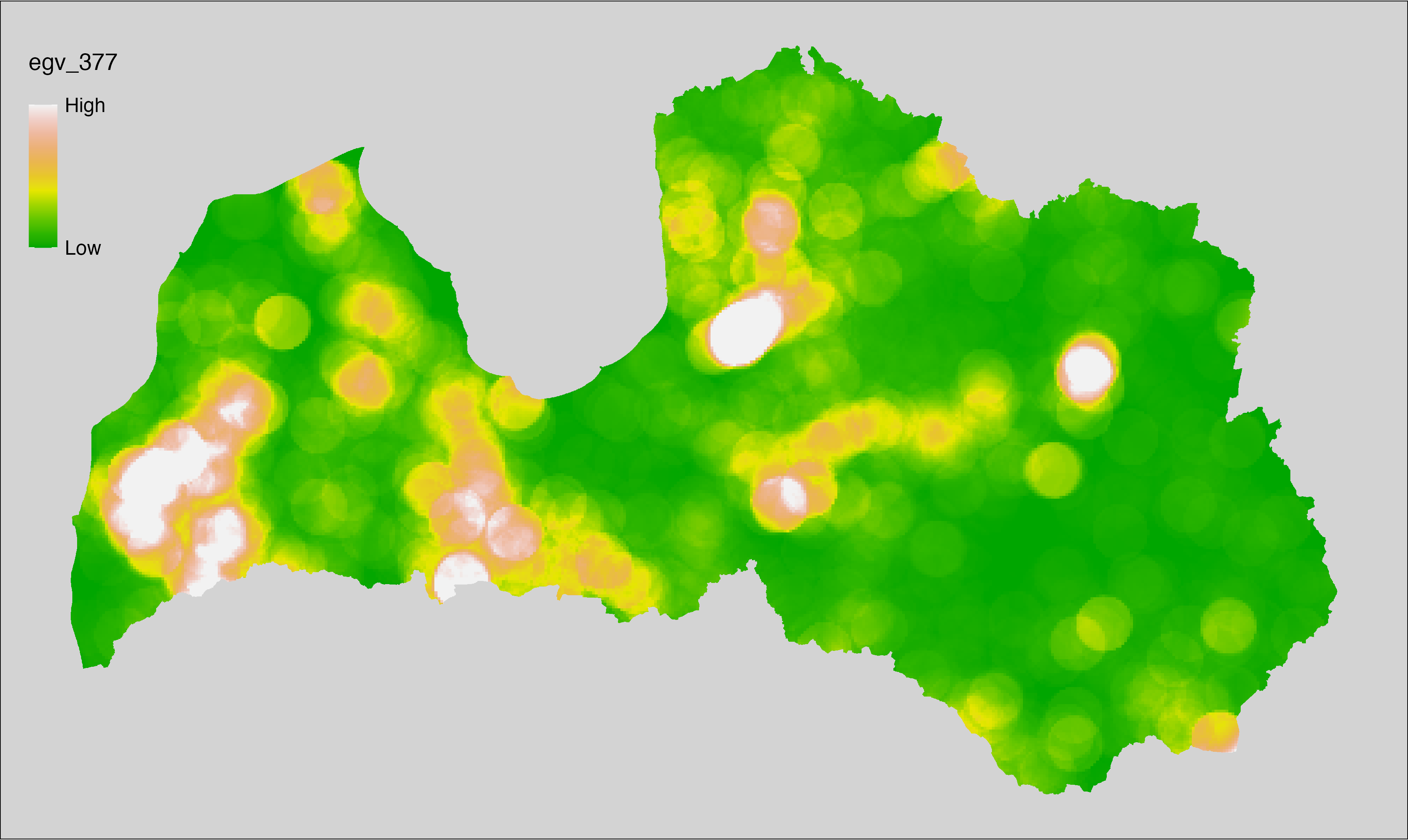
6.378 ForestsTreesAge_TemperateDeciduousYoung_cell
filename: ForestsTreesAge_TemperateDeciduousYoung_cell.tif
layername: egv_378
English name: Fractional cover of Young (pre-rotation age) Temperate Deciduous Forests within the analysis cell (1 ha)
Latvian name: Jaunu (pirms cirtmeta) platlapju mežu platības īpatsvars analīzes šūnā (1 ha)
Procedure: Most EGVs describing forests are spatially restricted to areas outside of clearcuts and dead stands. This mask is created using a combination of the State Forest Service’s State Forest Registry land category 12 and 14, and The Global Forest Watch pixels classified as lost tree canopy cover since 2020 (raster layer matching input, presence = 1, absence = 0).
To prepare this EGV, stands from the State Forest Service’s State Forest Registry are classified into (in order):
coniferous (see Terminology and acronyms for species codes) if timber volume of those species exceeded 75%;
Boreal deciduous if timber volume of those species exceeded 75%;
temperate deciduous if timber volume of those species exceeded 50%;
mixed otherwise;
then temperate deciduous stands younger than the legal rotation age are
selected and geometries are rasterised (presence = 1, NA otherwise). Rasterisation is
performed using the workflow egvtools::polygon2input(), restricting to pixels outside clearcut
mask and covering background with value 0. The resulting layer
is then aggregated to EGV resolution using the workflow egvtools::input2egv(), which
calculates the arithmetic mean to determine the cover fraction. During
aggregation, inverse distance weighted (power = 2) gap filling on the output is
applied to ensure no missing values at the edges. Finally, the layer is
standardised by subtracting the arithmetic mean and dividing by the root mean squared
error.
Code
# libs ----
if(!require(egvtools)) {remotes::install_github("aavotins/egvtools"); require(egvtools)}
if(!require(terra)) {install.packages("terra"); require(terra)}
if(!require(sf)) {install.packages("sf"); require(sf)}
if(!require(tidyverse)) {install.packages("tidyverse"); require(tidyverse)}
if(!require(sfarrow)) {install.packages("sfarrow"); require(sfarrow)}
if(!require(readxl)) {install.packages("readxl"); require(readxl)}
if(!require(raster)) {install.packages("raster"); require(raster)}
if(!require(fasterize)) {install.packages("fasterize"); require(fasterize)}
# templates ----
template100=rast("./Templates/TemplateRasters/LV100m_10km.tif")
template10=rast("./Templates/TemplateRasters/LV10m_10km.tif")
rastrs10=raster(template10)
nulls10=rast("./Templates/TemplateRasters/nulls_LV10m_10km.tif")
nulls100=rast("./Templates/TemplateRasters/nulls_LV100m_10km.tif")
# simple landscape ----
simple_landscape=rast("RasterGrids_10m/2024/Ainava_vienk_mask.tif")
# mvr ----
mvr=st_read_parquet("./Geodata/2024/MVR/nogabali_2024janv.parquet")
mvr$yes=1
# clear cut mask ----
izcirtumi=mvr %>%
filter(zkat %in% c("12","14")) %>%
dplyr::select(yes)
r_izcirtumi_mvr=fasterize(izcirtumi,rastrs10,field="yes")
t_izcirtumi_mvr=rast(r_izcirtumi_mvr)
plot(t_izcirtumi_mvr)
tcl=rast("./Geodata/2024/Trees/GFW/TreeCoverLoss_v1_12.tif")
tcl2=ifel(tcl<20,0,1)
tclX=cover(tcl2,nulls10)
plot(tclX)
clearcut_mask=cover(t_izcirtumi_mvr,tclX,
filename="./RasterGrids_10m/2024/Mask_clearcuts.tif",
overwrite=TRUE)
plot(clearcut_mask)
rm(izcirtumi)
rm(r_izcirtumi_mvr)
rm(t_izcirtumi_mvr)
rm(tcl)
rm(tcl2)
rm(tclX)
# ForestsTreesAge_TemperateDeciduousYoung_cell.tif egv_378 ----
skujkoki=c("1","3","13","14","15","22","23","28") # 8
saurlapji=c("4","6","8","9","19","20","21","32","35","68") # 10
platlapji=c("10","11","12","16","17","18","24","25","26","27","28","29","50",
"61","62","63","64","65","66","67","69") # 21
mvr=mvr %>%
mutate(kraja_skujkoku=ifelse(s10 %in% skujkoki,v10,0)+
ifelse(s11 %in% skujkoki,v11,0)+ifelse(s12 %in% skujkoki,v12,0)+
ifelse(s13 %in% skujkoki,v13,0)+ifelse(s14 %in% skujkoki,v14,0),
kraja_saurlapju=ifelse(s10 %in% saurlapji,v10,0)+
ifelse(s11 %in% saurlapji,v11,0)+ifelse(s12 %in% saurlapji,v12,0)+
ifelse(s13 %in% saurlapji,v13,0)+ifelse(s14 %in% saurlapji,v14,0),
kraja_platlapju=ifelse(s10 %in% platlapji,v10,0)+
ifelse(s11 %in% platlapji,v11,0)+ifelse(s12 %in% platlapji,v12,0)+
ifelse(s13 %in% platlapji,v13,0)+ifelse(s14 %in% platlapji,v14,0)) %>%
mutate(kopeja_kraja=kraja_skujkoku+kraja_platlapju+kraja_saurlapju) %>%
mutate(tips=ifelse(kraja_skujkoku/kopeja_kraja>=0.75,"skujkoku",
ifelse(kraja_saurlapju/kopeja_kraja>=0.75,"saurlapju",
ifelse(kraja_platlapju/kopeja_kraja>0.5,"platlapju",
"jauktu koku"))))
nogabali=mvr %>%
filter(zkat=="10"&tips=="platlapju"&(vgr=="1"|vgr=="2"|vgr=="3"))
p2i_rez=egvtools::polygon2input(vector_data = nogabali,
template_path = "./Templates/TemplateRasters/LV10m_10km.tif",
out_path = "./RasterGrids_10m/2024/",
file_name = "ForestsTreesAge_TemperateDeciduousYoung_input.tif",
value_field = "yes",
restrict_to = clearcut_mask,
restrict_values = 0,
prepare=FALSE,
background_raster = "./Templates/TemplateRasters/nulls_LV10m_10km.tif",
plot_result = TRUE)
p2i_rez
i2e_rez=egvtools::input2egv(input=paste0("./RasterGrids_10m/2024/",
"ForestsTreesAge_TemperateDeciduousYoung_input.tif"),
egv_template= "./Templates/TemplateRasters/LV100m_10km.tif",
summary_function = "average",
missing_job = "FillOutput",
outlocation = "./RasterGrids_100m/2024/RAW/",
outfilename = "ForestsTreesAge_TemperateDeciduousYoung_cell.tif",
layername = "egv_378",
idw_weight = 2,
plot_gaps = FALSE,plot_final = TRUE)
i2e_rez
rm(nogabali)
rm(p2i_rez)
rm(i2e_rez)
unlink("./RasterGrids_10m/2024/ForestsTreesAge_TemperateDeciduousYoung_input.tif")
# standardisation ----
if(!require(terra)) {install.packages("terra"); require(terra)}
if(!require(tidyverse)) {install.packages("tidyverse"); require(tidyverse)}
nosaukums="ForestsTreesAge_TemperateDeciduousYoung_cell.tif"
ielasisanas_cels=paste0("./RasterGrids_100m/2024/RAW/",nosaukums)
saglabasanas_cels=paste0("./RasterGrids_100m/2024/Scaled/",nosaukums)
slanis=rast(ielasisanas_cels)
videjais=global(slanis,fun="mean",na.rm=TRUE)
centrets=slanis-videjais[,1]
standartnovirze=terra::global(centrets,fun="rms",na.rm=TRUE)
merogots=centrets/standartnovirze[,1]
writeRaster(merogots,
filename=saglabasanas_cels,
overwrite=TRUE)
6.379 ForestsTreesAge_TemperateDeciduousYoung_r500
filename: ForestsTreesAge_TemperateDeciduousYoung_r500.tif
layername: egv_379
English name: Fractional cover of Young (pre-rotation age) Temperate Deciduous Forests within the 0.5 km landscape
Latvian name: Jaunu (pirms cirtmeta) platlapju mežu platības īpatsvars 0,5 km ainavā
Procedure: The cover fraction within a radius of 500 m around the analysis grid cell is
calculated as the area-weighted sum of the analysis cells inside the
buffer, using the workflow egvtools::radius_function(). During the calculation of the landscape metric,
inverse distance weighted (power = 2) gap filling on the output is applied
to ensure no missing values at the edges. Then the layer is rewritten to set
its name. Finally, the layer is standardised by subtracting the arithmetic
mean and dividing by the root mean squared error.
Code
# libs ----
if(!require(terra)) {install.packages("terra"); require(terra)}
if(!require(egvtools)) {remotes::install_github("aavotins/egvtools"); require(egvtools)}
# Templates -----
template100=rast("./Templates/TemplateRasters/LV100m_10km.tif")
# radii ----
radius_function(
kvadrati_path = "./Templates/TemplateGrids/tiles/",
radii_path = "./Templates/TemplateGridPoints/tiles/",
tikls100_path = "./Templates/TemplateGrids/tikls100_sauzeme.parquet",
template_path = "./Templates/TemplateRasters/LV100m_10km.tif",
input_layers = c("./RasterGrids_100m/2024/RAW/ForestsTreesAge_TemperateDeciduousYoung_cell.tif"),
layer_prefixes = c("ForestsTreesAge_TemperateDeciduousYoung"),
output_dir = "./RasterGrids_100m/2024/RAW/",
n_workers = 6,
radii = c("r500"),
radius_mode = "sparse",
extract_fun = "mean",
fill_missing = TRUE,
IDW_weight = 2,
future_max_size = 40 * 1024^3)
# ForestsTreesAge_TemperateDeciduousYoung_r500.tif egv_379
slanis=rast("./RasterGrids_100m/2024/RAW/ForestsTreesAge_TemperateDeciduousYoung_r500.tif")
names(slanis)="egv_379"
slanis2=project(slanis,template100)
writeRaster(slanis2,
"./RasterGrids_100m/2024/RAW/ForestsTreesAge_TemperateDeciduousYoung_r500.tif",
overwrite=TRUE)
# standardisation ----
if(!require(terra)) {install.packages("terra"); require(terra)}
if(!require(tidyverse)) {install.packages("tidyverse"); require(tidyverse)}
nosaukums="ForestsTreesAge_TemperateDeciduousYoung_r500.tif"
ielasisanas_cels=paste0("./RasterGrids_100m/2024/RAW/",nosaukums)
saglabasanas_cels=paste0("./RasterGrids_100m/2024/Scaled/",nosaukums)
slanis=rast(ielasisanas_cels)
videjais=global(slanis,fun="mean",na.rm=TRUE)
centrets=slanis-videjais[,1]
standartnovirze=terra::global(centrets,fun="rms",na.rm=TRUE)
merogots=centrets/standartnovirze[,1]
writeRaster(merogots,
filename=saglabasanas_cels,
overwrite=TRUE)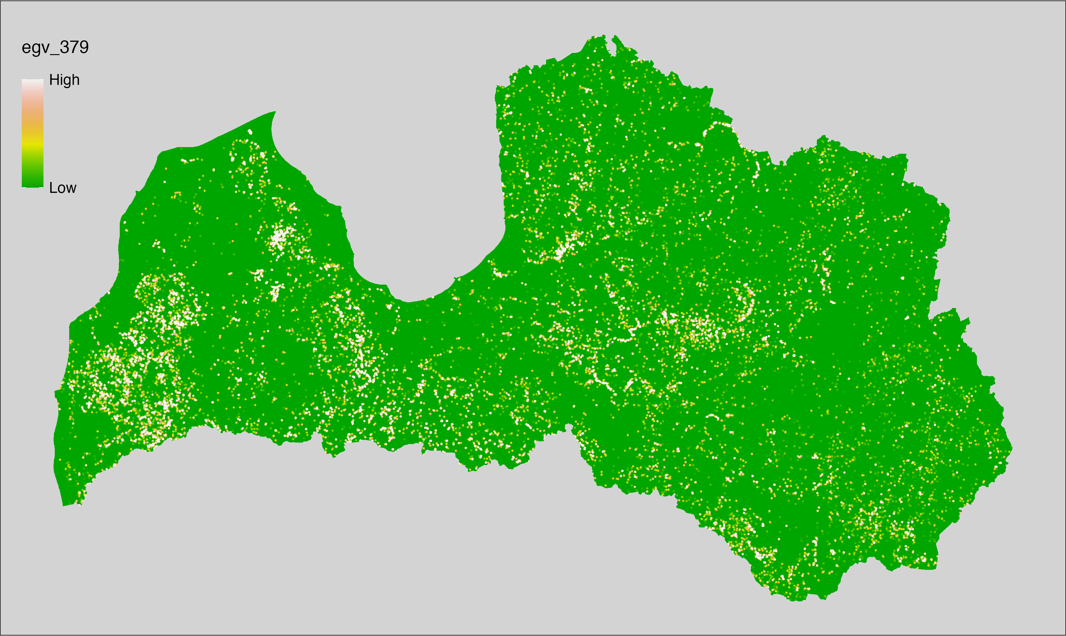
6.380 ForestsTreesAge_TemperateDeciduousYoung_r1250
filename: ForestsTreesAge_TemperateDeciduousYoung_r1250.tif
layername: egv_380
English name: Fractional cover of Young (pre-rotation age) Temperate Deciduous Forests within the 1.25 km landscape
Latvian name: Jaunu (pirms cirtmeta) platlapju mežu platības īpatsvars 1,25 km ainavā
Procedure: The cover fraction within a radius of 1250 m around the analysis grid cell
is calculated as the area-weighted sum of the analysis cells inside
the buffer, using the workflow egvtools::radius_function(). During the calculation of the landscape
metric, inverse distance weighted (power = 2) gap filling on the output is
applied to ensure no missing values at the edges. Then the layer is
rewritten to set its name. Finally, the layer is standardised by
subtracting the arithmetic mean and dividing by the root mean squared error.
Code
# libs ----
if(!require(terra)) {install.packages("terra"); require(terra)}
if(!require(egvtools)) {remotes::install_github("aavotins/egvtools"); require(egvtools)}
# Templates -----
template100=rast("./Templates/TemplateRasters/LV100m_10km.tif")
# radii ----
radius_function(
kvadrati_path = "./Templates/TemplateGrids/tiles/",
radii_path = "./Templates/TemplateGridPoints/tiles/",
tikls100_path = "./Templates/TemplateGrids/tikls100_sauzeme.parquet",
template_path = "./Templates/TemplateRasters/LV100m_10km.tif",
input_layers = c("./RasterGrids_100m/2024/RAW/ForestsTreesAge_TemperateDeciduousYoung_cell.tif"),
layer_prefixes = c("ForestsTreesAge_TemperateDeciduousYoung"),
output_dir = "./RasterGrids_100m/2024/RAW/",
n_workers = 6,
radii = c("r1250"),
radius_mode = "sparse",
extract_fun = "mean",
fill_missing = TRUE,
IDW_weight = 2,
future_max_size = 40 * 1024^3)
# ForestsTreesAge_TemperateDeciduousYoung_r1250.tif egv_380
slanis=rast("./RasterGrids_100m/2024/RAW/ForestsTreesAge_TemperateDeciduousYoung_r1250.tif")
names(slanis)="egv_380"
slanis2=project(slanis,template100)
writeRaster(slanis2,
"./RasterGrids_100m/2024/RAW/ForestsTreesAge_TemperateDeciduousYoung_r1250.tif",
overwrite=TRUE)
# standardisation ----
if(!require(terra)) {install.packages("terra"); require(terra)}
if(!require(tidyverse)) {install.packages("tidyverse"); require(tidyverse)}
nosaukums="ForestsTreesAge_TemperateDeciduousYoung_r1250.tif"
ielasisanas_cels=paste0("./RasterGrids_100m/2024/RAW/",nosaukums)
saglabasanas_cels=paste0("./RasterGrids_100m/2024/Scaled/",nosaukums)
slanis=rast(ielasisanas_cels)
videjais=global(slanis,fun="mean",na.rm=TRUE)
centrets=slanis-videjais[,1]
standartnovirze=terra::global(centrets,fun="rms",na.rm=TRUE)
merogots=centrets/standartnovirze[,1]
writeRaster(merogots,
filename=saglabasanas_cels,
overwrite=TRUE)
6.381 ForestsTreesAge_TemperateDeciduousYoung_r3000
filename: ForestsTreesAge_TemperateDeciduousYoung_r3000.tif
layername: egv_381
English name: Fractional cover of Young (pre-rotation age) Temperate Deciduous Forests within the 3 km landscape
Latvian name: Jaunu (pirms cirtmeta) platlapju mežu platības īpatsvars 3 km ainavā
Procedure: The cover fraction within a radius of 3000 m around the analysis grid cell
is calculated as the area-weighted sum of the analysis cells inside
the buffer, using the workflow egvtools::radius_function(). During the calculation of the landscape
metric, inverse distance weighted (power = 2) gap filling on the output is
applied to ensure no missing values at the edges. Then the layer is
rewritten to set its name. Finally, the layer is standardised by
subtracting the arithmetic mean and dividing by the root mean squared error.
Code
# libs ----
if(!require(terra)) {install.packages("terra"); require(terra)}
if(!require(egvtools)) {remotes::install_github("aavotins/egvtools"); require(egvtools)}
# Templates -----
template100=rast("./Templates/TemplateRasters/LV100m_10km.tif")
# radii ----
radius_function(
kvadrati_path = "./Templates/TemplateGrids/tiles/",
radii_path = "./Templates/TemplateGridPoints/tiles/",
tikls100_path = "./Templates/TemplateGrids/tikls100_sauzeme.parquet",
template_path = "./Templates/TemplateRasters/LV100m_10km.tif",
input_layers = c("./RasterGrids_100m/2024/RAW/ForestsTreesAge_TemperateDeciduousYoung_cell.tif"),
layer_prefixes = c("ForestsTreesAge_TemperateDeciduousYoung"),
output_dir = "./RasterGrids_100m/2024/RAW/",
n_workers = 6,
radii = c("r3000"),
radius_mode = "sparse",
extract_fun = "mean",
fill_missing = TRUE,
IDW_weight = 2,
future_max_size = 40 * 1024^3)
# ForestsTreesAge_TemperateDeciduousYoung_r3000.tif egv_381
slanis=rast("./RasterGrids_100m/2024/RAW/ForestsTreesAge_TemperateDeciduousYoung_r3000.tif")
names(slanis)="egv_381"
slanis2=project(slanis,template100)
writeRaster(slanis2,
"./RasterGrids_100m/2024/RAW/ForestsTreesAge_TemperateDeciduousYoung_r3000.tif",
overwrite=TRUE)
# standardisation ----
if(!require(terra)) {install.packages("terra"); require(terra)}
if(!require(tidyverse)) {install.packages("tidyverse"); require(tidyverse)}
nosaukums="ForestsTreesAge_TemperateDeciduousYoung_r3000.tif"
ielasisanas_cels=paste0("./RasterGrids_100m/2024/RAW/",nosaukums)
saglabasanas_cels=paste0("./RasterGrids_100m/2024/Scaled/",nosaukums)
slanis=rast(ielasisanas_cels)
videjais=global(slanis,fun="mean",na.rm=TRUE)
centrets=slanis-videjais[,1]
standartnovirze=terra::global(centrets,fun="rms",na.rm=TRUE)
merogots=centrets/standartnovirze[,1]
writeRaster(merogots,
filename=saglabasanas_cels,
overwrite=TRUE)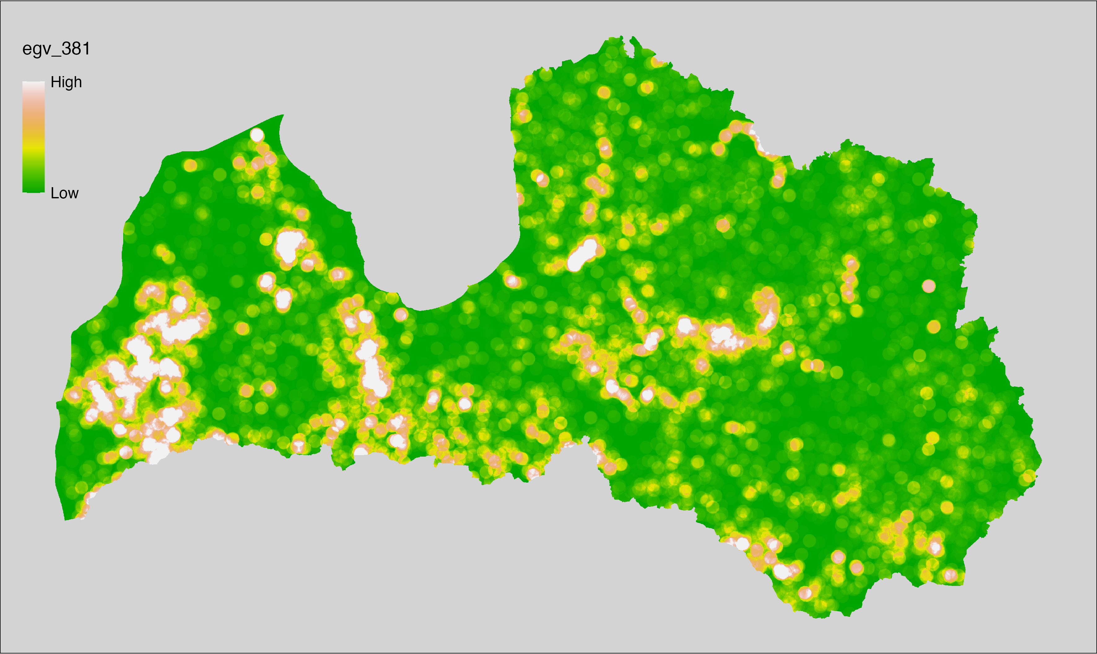
6.382 ForestsTreesAge_TemperateDeciduousYoung_r10000
filename: ForestsTreesAge_TemperateDeciduousYoung_r10000.tif
layername: egv_382
English name: Fractional cover of Young (pre-rotation age) Temperate Deciduous Forests within the 10 km landscape
Latvian name: Jaunu (pirms cirtmeta) platlapju mežu platības īpatsvars 10 km ainavā
Procedure: The cover fraction within a radius of 10000 m around the analysis grid cell
is calculated as the area-weighted sum of the analysis cells inside
the buffer, using the workflow egvtools::radius_function(). During the calculation of the landscape
metric, inverse distance weighted (power = 2) gap filling on the output is
applied to ensure no missing values at the edges. Then the layer is
rewritten to set its name. Finally, the layer is standardised by
subtracting the arithmetic mean and dividing by the root mean squared error.
Code
# libs ----
if(!require(terra)) {install.packages("terra"); require(terra)}
if(!require(egvtools)) {remotes::install_github("aavotins/egvtools"); require(egvtools)}
# Templates -----
template100=rast("./Templates/TemplateRasters/LV100m_10km.tif")
# radii ----
radius_function(
kvadrati_path = "./Templates/TemplateGrids/tiles/",
radii_path = "./Templates/TemplateGridPoints/tiles/",
tikls100_path = "./Templates/TemplateGrids/tikls100_sauzeme.parquet",
template_path = "./Templates/TemplateRasters/LV100m_10km.tif",
input_layers = c("./RasterGrids_100m/2024/RAW/ForestsTreesAge_TemperateDeciduousYoung_cell.tif"),
layer_prefixes = c("ForestsTreesAge_TemperateDeciduousYoung"),
output_dir = "./RasterGrids_100m/2024/RAW/",
n_workers = 6,
radii = c("r10000"),
radius_mode = "sparse",
extract_fun = "mean",
fill_missing = TRUE,
IDW_weight = 2,
future_max_size = 40 * 1024^3)
# ForestsTreesAge_TemperateDeciduousYoung_r10000.tif egv_382
slanis=rast("./RasterGrids_100m/2024/RAW/ForestsTreesAge_TemperateDeciduousYoung_r10000.tif")
names(slanis)="egv_382"
slanis2=project(slanis,template100)
writeRaster(slanis2,
"./RasterGrids_100m/2024/RAW/ForestsTreesAge_TemperateDeciduousYoung_r10000.tif",
overwrite=TRUE)
# standardisation ----
if(!require(terra)) {install.packages("terra"); require(terra)}
if(!require(tidyverse)) {install.packages("tidyverse"); require(tidyverse)}
nosaukums="ForestsTreesAge_TemperateDeciduousYoung_r10000.tif"
ielasisanas_cels=paste0("./RasterGrids_100m/2024/RAW/",nosaukums)
saglabasanas_cels=paste0("./RasterGrids_100m/2024/Scaled/",nosaukums)
slanis=rast(ielasisanas_cels)
videjais=global(slanis,fun="mean",na.rm=TRUE)
centrets=slanis-videjais[,1]
standartnovirze=terra::global(centrets,fun="rms",na.rm=TRUE)
merogots=centrets/standartnovirze[,1]
writeRaster(merogots,
filename=saglabasanas_cels,
overwrite=TRUE)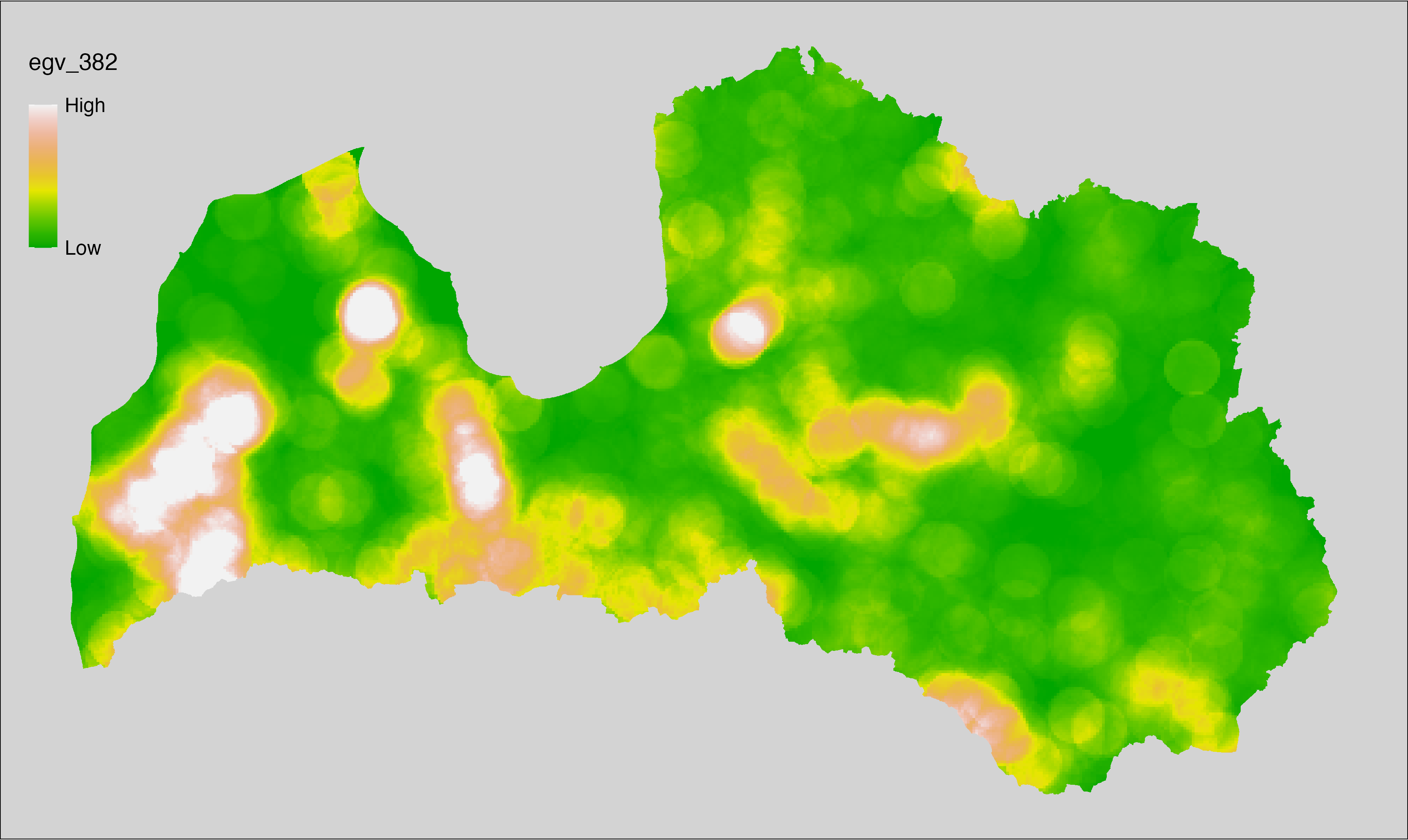
6.383 ForestsTrees_BorealDeciduous_cell
filename: ForestsTrees_BorealDeciduous_cell.tif
layername: egv_383
English name: Fractional cover of Boreal Deciduous Forests within the analysis cell (1 ha)
Latvian name: Šaurlapju mežu platības īpatsvars analīzes šūnā (1 ha)
Procedure: Most EGVs describing forests are spatially restricted to areas outside of clearcuts and dead stands. This mask is created using a combination of the State Forest Service’s State Forest Registry land category 12 and 14, and The Global Forest Watch pixels classified as lost tree canopy cover since 2020 (raster layer matching input, presence = 1, absence = 0).
To prepare this EGV, stands from the State Forest Service’s State Forest Registry are classified into (in order):
coniferous (see Terminology and acronyms for species codes) if timber volume of those species exceeded 75%;
Boreal deciduous if timber volume of those species exceeded 75%;
temperate deciduous if timber volume of those species exceeded 50%;
mixed otherwise;
then Boreal deciduous stands are selected and geometries are
rasterised (presence = 1, NA otherwise). Rasterisation is
performed using the workflow egvtools::polygon2input(), restricting to pixels outside clearcut
mask and covering background with value 0. The resulting layer
is then aggregated to EGV resolution using the workflow egvtools::input2egv(), which
calculates the arithmetic mean to determine the cover fraction. During
aggregation, inverse distance weighted (power = 2) gap filling on the output is
applied to ensure no missing values at the edges. Finally, the layer is
standardised by subtracting the arithmetic mean and dividing by the root mean squared
error.
Code
# libs ----
if(!require(egvtools)) {remotes::install_github("aavotins/egvtools"); require(egvtools)}
if(!require(terra)) {install.packages("terra"); require(terra)}
if(!require(sf)) {install.packages("sf"); require(sf)}
if(!require(tidyverse)) {install.packages("tidyverse"); require(tidyverse)}
if(!require(sfarrow)) {install.packages("sfarrow"); require(sfarrow)}
if(!require(readxl)) {install.packages("readxl"); require(readxl)}
if(!require(raster)) {install.packages("raster"); require(raster)}
if(!require(fasterize)) {install.packages("fasterize"); require(fasterize)}
# templates ----
template100=rast("./Templates/TemplateRasters/LV100m_10km.tif")
template10=rast("./Templates/TemplateRasters/LV10m_10km.tif")
rastrs10=raster(template10)
nulls10=rast("./Templates/TemplateRasters/nulls_LV10m_10km.tif")
nulls100=rast("./Templates/TemplateRasters/nulls_LV100m_10km.tif")
# simple landscape ----
simple_landscape=rast("RasterGrids_10m/2024/Ainava_vienk_mask.tif")
# mvr ----
mvr=st_read_parquet("./Geodata/2024/MVR/nogabali_2024janv.parquet")
mvr$yes=1
# clear cut mask ----
izcirtumi=mvr %>%
filter(zkat %in% c("12","14")) %>%
dplyr::select(yes)
r_izcirtumi_mvr=fasterize(izcirtumi,rastrs10,field="yes")
t_izcirtumi_mvr=rast(r_izcirtumi_mvr)
plot(t_izcirtumi_mvr)
tcl=rast("./Geodata/2024/Trees/GFW/TreeCoverLoss_v1_12.tif")
tcl2=ifel(tcl<20,0,1)
tclX=cover(tcl2,nulls10)
plot(tclX)
clearcut_mask=cover(t_izcirtumi_mvr,tclX,
filename="./RasterGrids_10m/2024/Mask_clearcuts.tif",
overwrite=TRUE)
plot(clearcut_mask)
rm(izcirtumi)
rm(r_izcirtumi_mvr)
rm(t_izcirtumi_mvr)
rm(tcl)
rm(tcl2)
rm(tclX)
# ForestsTrees_BorealDeciduous_cell.tif egv_383 ----
skujkoki=c("1","3","13","14","15","22","23","28") # 8
saurlapji=c("4","6","8","9","19","20","21","32","35","68") # 10
platlapji=c("10","11","12","16","17","18","24","25","26","27","28","29","50",
"61","62","63","64","65","66","67","69") # 21
mvr=mvr %>%
mutate(kraja_skujkoku=ifelse(s10 %in% skujkoki,v10,0)+
ifelse(s11 %in% skujkoki,v11,0)+ifelse(s12 %in% skujkoki,v12,0)+
ifelse(s13 %in% skujkoki,v13,0)+ifelse(s14 %in% skujkoki,v14,0),
kraja_saurlapju=ifelse(s10 %in% saurlapji,v10,0)+
ifelse(s11 %in% saurlapji,v11,0)+ifelse(s12 %in% saurlapji,v12,0)+
ifelse(s13 %in% saurlapji,v13,0)+ifelse(s14 %in% saurlapji,v14,0),
kraja_platlapju=ifelse(s10 %in% platlapji,v10,0)+
ifelse(s11 %in% platlapji,v11,0)+ifelse(s12 %in% platlapji,v12,0)+
ifelse(s13 %in% platlapji,v13,0)+ifelse(s14 %in% platlapji,v14,0)) %>%
mutate(kopeja_kraja=kraja_skujkoku+kraja_platlapju+kraja_saurlapju) %>%
mutate(tips=ifelse(kraja_skujkoku/kopeja_kraja>=0.75,"skujkoku",
ifelse(kraja_saurlapju/kopeja_kraja>=0.75,"saurlapju",
ifelse(kraja_platlapju/kopeja_kraja>0.5,"platlapju",
"jauktu koku"))))
nogabali=mvr %>%
filter(zkat=="10"&tips=="saurlapju")
p2i_rez=egvtools::polygon2input(vector_data = nogabali,
template_path = "./Templates/TemplateRasters/LV10m_10km.tif",
out_path = "./RasterGrids_10m/2024/",
file_name = "ForestsTrees_BorealDeciduous_input.tif",
value_field = "yes",
restrict_to = clearcut_mask,
restrict_values = 0,
prepare=FALSE,
background_raster = "./Templates/TemplateRasters/nulls_LV10m_10km.tif",
plot_result = TRUE)
p2i_rez
i2e_rez=egvtools::input2egv(input=paste0("./RasterGrids_10m/2024/",
"ForestsTrees_BorealDeciduous_input.tif"),
egv_template= "./Templates/TemplateRasters/LV100m_10km.tif",
summary_function = "average",
missing_job = "FillOutput",
outlocation = "./RasterGrids_100m/2024/RAW/",
outfilename = "ForestsTrees_BorealDeciduous_cell.tif",
layername = "egv_383",
idw_weight = 2,
plot_gaps = FALSE,plot_final = TRUE)
i2e_rez
rm(nogabali)
rm(p2i_rez)
rm(i2e_rez)
unlink("./RasterGrids_10m/2024/ForestsTrees_BorealDeciduous_input.tif")
# standardisation ----
if(!require(terra)) {install.packages("terra"); require(terra)}
if(!require(tidyverse)) {install.packages("tidyverse"); require(tidyverse)}
nosaukums="ForestsTrees_BorealDeciduous_cell.tif"
ielasisanas_cels=paste0("./RasterGrids_100m/2024/RAW/",nosaukums)
saglabasanas_cels=paste0("./RasterGrids_100m/2024/Scaled/",nosaukums)
slanis=rast(ielasisanas_cels)
videjais=global(slanis,fun="mean",na.rm=TRUE)
centrets=slanis-videjais[,1]
standartnovirze=terra::global(centrets,fun="rms",na.rm=TRUE)
merogots=centrets/standartnovirze[,1]
writeRaster(merogots,
filename=saglabasanas_cels,
overwrite=TRUE)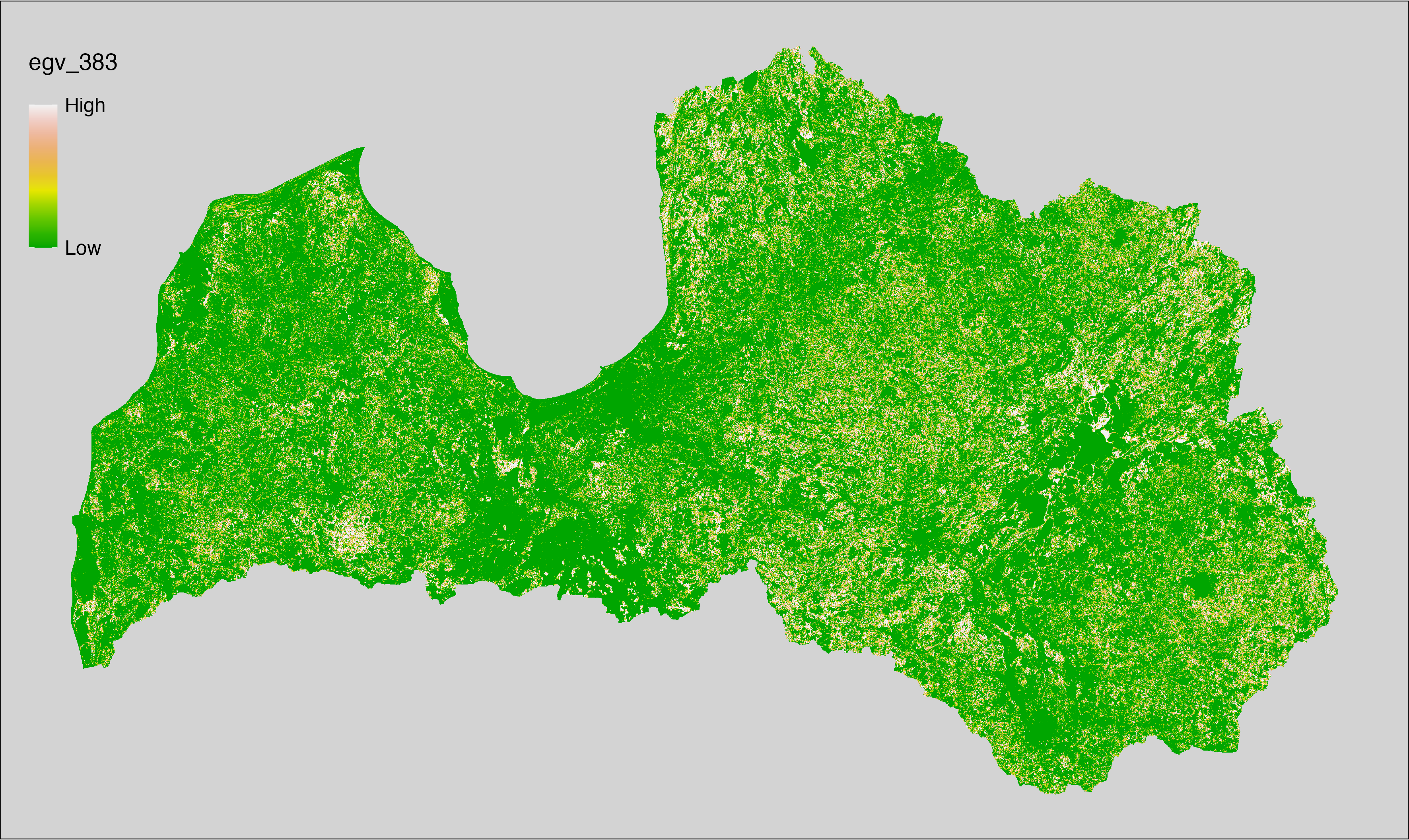
6.384 ForestsTrees_BorealDeciduous_r500
filename: ForestsTrees_BorealDeciduous_r500.tif
layername: egv_384
English name: Fractional cover of Boreal Deciduous Forests within the 0.5 km landscape
Latvian name: Šaurlapju mežu platības īpatsvars 0,5 km ainavā
Procedure: The cover fraction within a radius of 500 m around the analysis grid cell is
calculated as the area-weighted sum of the analysis cells inside the
buffer, using the workflow egvtools::radius_function(). During the calculation of the landscape metric,
inverse distance weighted (power = 2) gap filling on the output is applied
to ensure no missing values at the edges. Then the layer is rewritten to set
its name. Finally, the layer is standardised by subtracting the arithmetic
mean and dividing by the root mean squared error.
Code
# libs ----
if(!require(terra)) {install.packages("terra"); require(terra)}
if(!require(egvtools)) {remotes::install_github("aavotins/egvtools"); require(egvtools)}
# Templates -----
template100=rast("./Templates/TemplateRasters/LV100m_10km.tif")
# radii ----
radius_function(
kvadrati_path = "./Templates/TemplateGrids/tiles/",
radii_path = "./Templates/TemplateGridPoints/tiles/",
tikls100_path = "./Templates/TemplateGrids/tikls100_sauzeme.parquet",
template_path = "./Templates/TemplateRasters/LV100m_10km.tif",
input_layers = c("./RasterGrids_100m/2024/RAW/ForestsTrees_BorealDeciduous_cell.tif"),
layer_prefixes = c("ForestsTrees_BorealDeciduous"),
output_dir = "./RasterGrids_100m/2024/RAW/",
n_workers = 6,
radii = c("r500"),
radius_mode = "sparse",
extract_fun = "mean",
fill_missing = TRUE,
IDW_weight = 2,
future_max_size = 40 * 1024^3)
# ForestsTrees_BorealDeciduous_r500.tif egv_384
slanis=rast("./RasterGrids_100m/2024/RAW/ForestsTrees_BorealDeciduous_r500.tif")
names(slanis)="egv_384"
slanis2=project(slanis,template100)
writeRaster(slanis2,
"./RasterGrids_100m/2024/RAW/ForestsTrees_BorealDeciduous_r500.tif",
overwrite=TRUE)
# standardisation ----
if(!require(terra)) {install.packages("terra"); require(terra)}
if(!require(tidyverse)) {install.packages("tidyverse"); require(tidyverse)}
nosaukums="ForestsTrees_BorealDeciduous_r500.tif"
ielasisanas_cels=paste0("./RasterGrids_100m/2024/RAW/",nosaukums)
saglabasanas_cels=paste0("./RasterGrids_100m/2024/Scaled/",nosaukums)
slanis=rast(ielasisanas_cels)
videjais=global(slanis,fun="mean",na.rm=TRUE)
centrets=slanis-videjais[,1]
standartnovirze=terra::global(centrets,fun="rms",na.rm=TRUE)
merogots=centrets/standartnovirze[,1]
writeRaster(merogots,
filename=saglabasanas_cels,
overwrite=TRUE)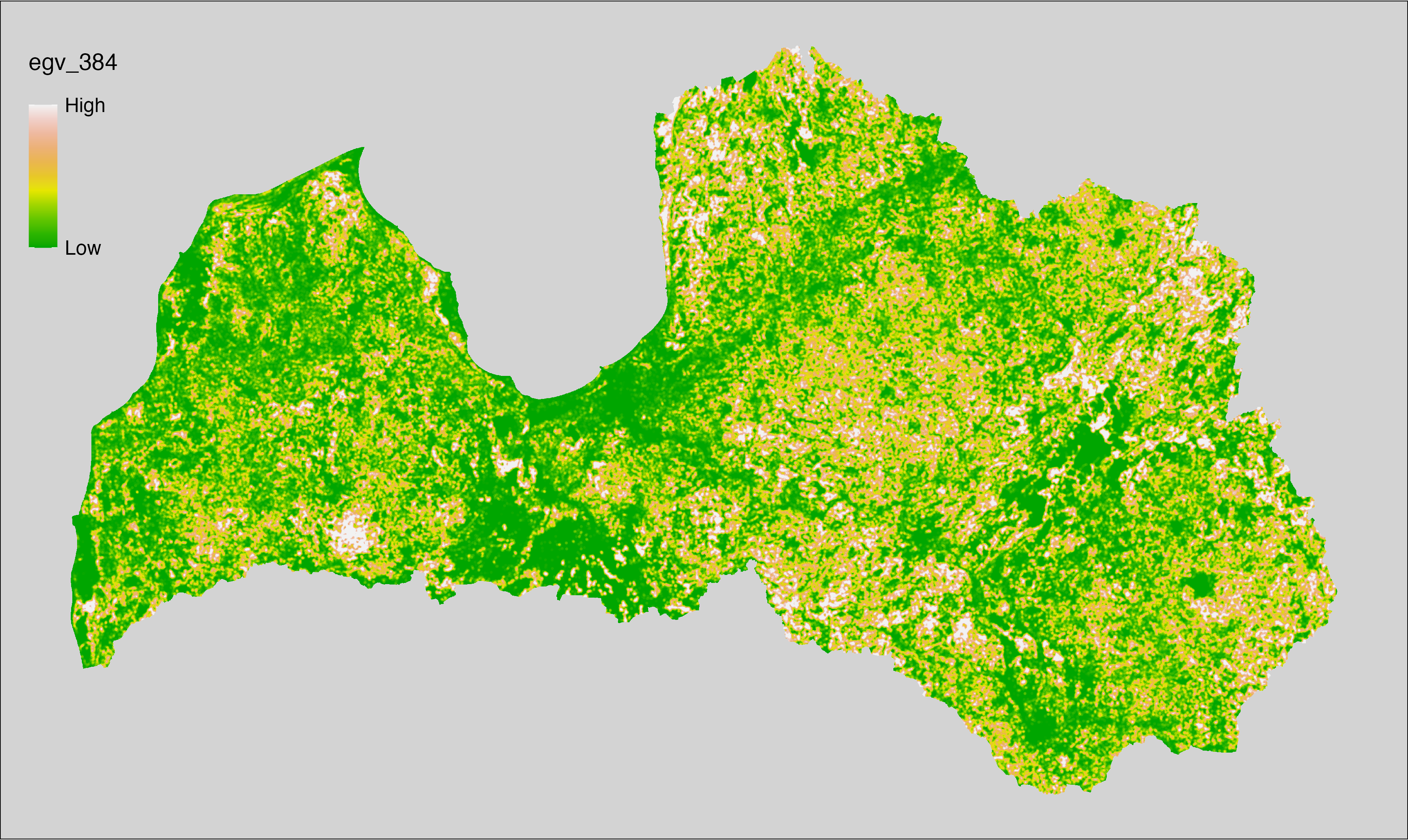
6.385 ForestsTrees_BorealDeciduous_r1250
filename: ForestsTrees_BorealDeciduous_r1250.tif
layername: egv_385
English name: Fractional cover of Boreal Deciduous Forests within the 1.25 km landscape
Latvian name: Šaurlapju mežu platības īpatsvars 1,25 km ainavā
Procedure: The cover fraction within a radius of 1250 m around the analysis grid cell
is calculated as the area-weighted sum of the analysis cells inside
the buffer, using the workflow egvtools::radius_function(). During the calculation of the landscape
metric, inverse distance weighted (power = 2) gap filling on the output is
applied to ensure no missing values at the edges. Then the layer is
rewritten to set its name. Finally, the layer is standardised by
subtracting the arithmetic mean and dividing by the root mean squared error.
Code
# libs ----
if(!require(terra)) {install.packages("terra"); require(terra)}
if(!require(egvtools)) {remotes::install_github("aavotins/egvtools"); require(egvtools)}
# Templates -----
template100=rast("./Templates/TemplateRasters/LV100m_10km.tif")
# radii ----
radius_function(
kvadrati_path = "./Templates/TemplateGrids/tiles/",
radii_path = "./Templates/TemplateGridPoints/tiles/",
tikls100_path = "./Templates/TemplateGrids/tikls100_sauzeme.parquet",
template_path = "./Templates/TemplateRasters/LV100m_10km.tif",
input_layers = c("./RasterGrids_100m/2024/RAW/ForestsTrees_BorealDeciduous_cell.tif"),
layer_prefixes = c("ForestsTrees_BorealDeciduous"),
output_dir = "./RasterGrids_100m/2024/RAW/",
n_workers = 6,
radii = c("r1250"),
radius_mode = "sparse",
extract_fun = "mean",
fill_missing = TRUE,
IDW_weight = 2,
future_max_size = 40 * 1024^3)
# ForestsTrees_BorealDeciduous_r1250.tif egv_385
slanis=rast("./RasterGrids_100m/2024/RAW/ForestsTrees_BorealDeciduous_r1250.tif")
names(slanis)="egv_385"
slanis2=project(slanis,template100)
writeRaster(slanis2,
"./RasterGrids_100m/2024/RAW/ForestsTrees_BorealDeciduous_r1250.tif",
overwrite=TRUE)
# standardisation ----
if(!require(terra)) {install.packages("terra"); require(terra)}
if(!require(tidyverse)) {install.packages("tidyverse"); require(tidyverse)}
nosaukums="ForestsTrees_BorealDeciduous_r1250.tif"
ielasisanas_cels=paste0("./RasterGrids_100m/2024/RAW/",nosaukums)
saglabasanas_cels=paste0("./RasterGrids_100m/2024/Scaled/",nosaukums)
slanis=rast(ielasisanas_cels)
videjais=global(slanis,fun="mean",na.rm=TRUE)
centrets=slanis-videjais[,1]
standartnovirze=terra::global(centrets,fun="rms",na.rm=TRUE)
merogots=centrets/standartnovirze[,1]
writeRaster(merogots,
filename=saglabasanas_cels,
overwrite=TRUE)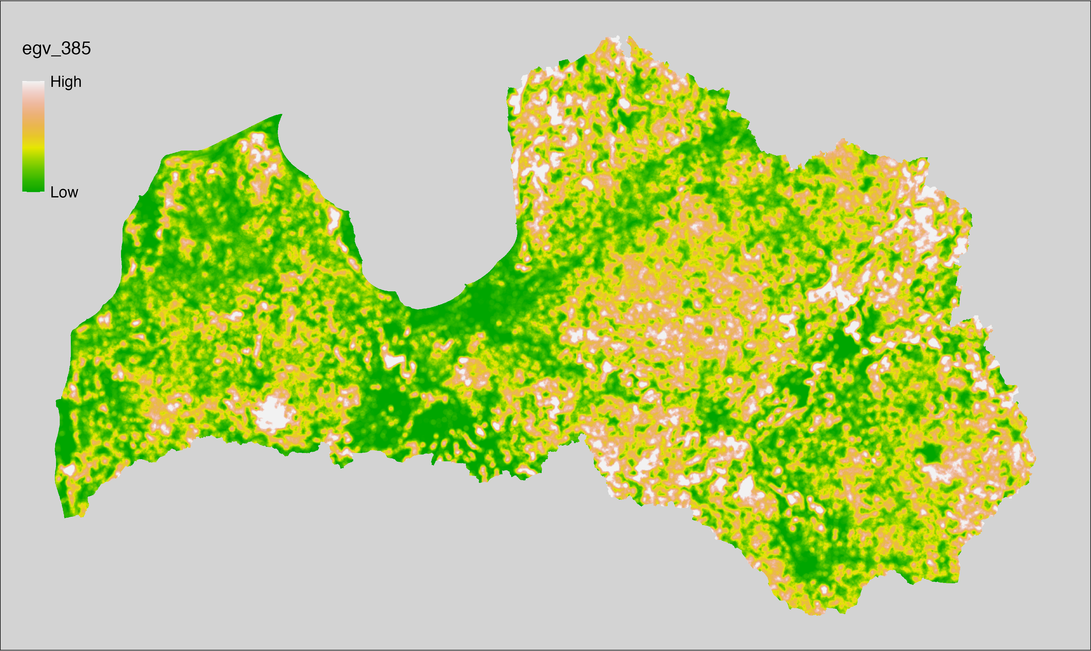
6.386 ForestsTrees_BorealDeciduous_r3000
filename: ForestsTrees_BorealDeciduous_r3000.tif
layername: egv_386
English name: Fractional cover of Boreal Deciduous Forests within the 3 km landscape
Latvian name: Šaurlapju mežu platības īpatsvars 3 km ainavā
Procedure: The cover fraction within a radius of 3000 m around the analysis grid cell
is calculated as the area-weighted sum of the analysis cells inside
the buffer, using the workflow egvtools::radius_function(). During the calculation of the landscape
metric, inverse distance weighted (power = 2) gap filling on the output is
applied to ensure no missing values at the edges. Then the layer is
rewritten to set its name. Finally, the layer is standardised by
subtracting the arithmetic mean and dividing by the root mean squared error.
Code
# libs ----
if(!require(terra)) {install.packages("terra"); require(terra)}
if(!require(egvtools)) {remotes::install_github("aavotins/egvtools"); require(egvtools)}
# Templates -----
template100=rast("./Templates/TemplateRasters/LV100m_10km.tif")
# radii ----
radius_function(
kvadrati_path = "./Templates/TemplateGrids/tiles/",
radii_path = "./Templates/TemplateGridPoints/tiles/",
tikls100_path = "./Templates/TemplateGrids/tikls100_sauzeme.parquet",
template_path = "./Templates/TemplateRasters/LV100m_10km.tif",
input_layers = c("./RasterGrids_100m/2024/RAW/ForestsTrees_BorealDeciduous_cell.tif"),
layer_prefixes = c("ForestsTrees_BorealDeciduous"),
output_dir = "./RasterGrids_100m/2024/RAW/",
n_workers = 6,
radii = c("r3000"),
radius_mode = "sparse",
extract_fun = "mean",
fill_missing = TRUE,
IDW_weight = 2,
future_max_size = 40 * 1024^3)
# ForestsTrees_BorealDeciduous_r3000.tif egv_386
slanis=rast("./RasterGrids_100m/2024/RAW/ForestsTrees_BorealDeciduous_r3000.tif")
names(slanis)="egv_386"
slanis2=project(slanis,template100)
writeRaster(slanis2,
"./RasterGrids_100m/2024/RAW/ForestsTrees_BorealDeciduous_r3000.tif",
overwrite=TRUE)
# standardisation ----
if(!require(terra)) {install.packages("terra"); require(terra)}
if(!require(tidyverse)) {install.packages("tidyverse"); require(tidyverse)}
nosaukums="ForestsTrees_BorealDeciduous_r3000.tif"
ielasisanas_cels=paste0("./RasterGrids_100m/2024/RAW/",nosaukums)
saglabasanas_cels=paste0("./RasterGrids_100m/2024/Scaled/",nosaukums)
slanis=rast(ielasisanas_cels)
videjais=global(slanis,fun="mean",na.rm=TRUE)
centrets=slanis-videjais[,1]
standartnovirze=terra::global(centrets,fun="rms",na.rm=TRUE)
merogots=centrets/standartnovirze[,1]
writeRaster(merogots,
filename=saglabasanas_cels,
overwrite=TRUE)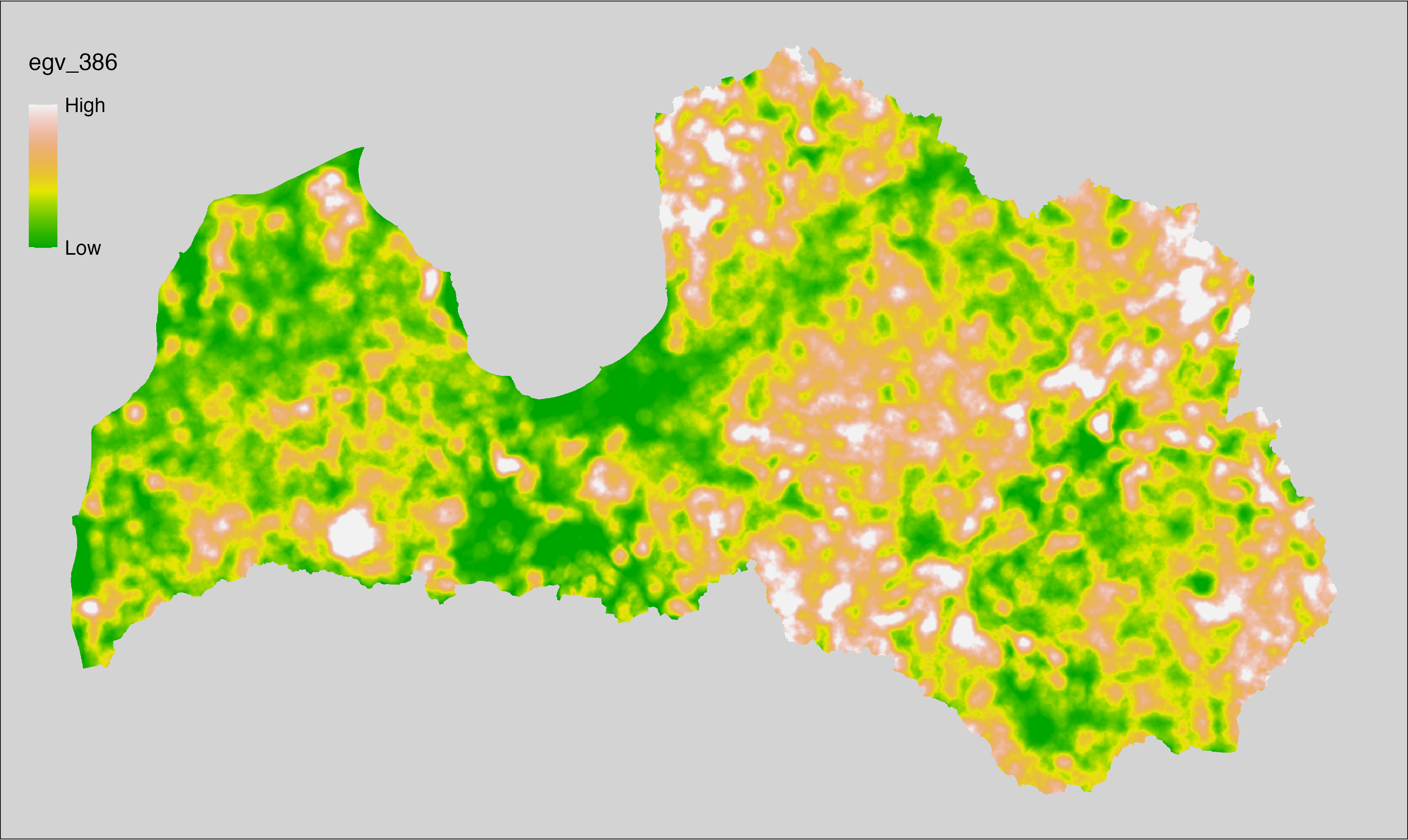
6.387 ForestsTrees_BorealDeciduous_r10000
filename: ForestsTrees_BorealDeciduous_r10000.tif
layername: egv_387
English name: Fractional cover of Boreal Deciduous Forests within the 10 km landscape
Latvian name: Šaurlapju mežu platības īpatsvars 10 km ainavā
Procedure: The cover fraction within a radius of 10000 m around the analysis grid cell
is calculated as the area-weighted sum of the analysis cells inside
the buffer, using the workflow egvtools::radius_function(). During the calculation of the landscape
metric, inverse distance weighted (power = 2) gap filling on the output is
applied to ensure no missing values at the edges. Then the layer is
rewritten to set its name. Finally, the layer is standardised by
subtracting the arithmetic mean and dividing by the root mean squared error.
Code
# libs ----
if(!require(terra)) {install.packages("terra"); require(terra)}
if(!require(egvtools)) {remotes::install_github("aavotins/egvtools"); require(egvtools)}
# Templates -----
template100=rast("./Templates/TemplateRasters/LV100m_10km.tif")
# radii ----
radius_function(
kvadrati_path = "./Templates/TemplateGrids/tiles/",
radii_path = "./Templates/TemplateGridPoints/tiles/",
tikls100_path = "./Templates/TemplateGrids/tikls100_sauzeme.parquet",
template_path = "./Templates/TemplateRasters/LV100m_10km.tif",
input_layers = c("./RasterGrids_100m/2024/RAW/ForestsTrees_BorealDeciduous_cell.tif"),
layer_prefixes = c("ForestsTrees_BorealDeciduous"),
output_dir = "./RasterGrids_100m/2024/RAW/",
n_workers = 6,
radii = c("r10000"),
radius_mode = "sparse",
extract_fun = "mean",
fill_missing = TRUE,
IDW_weight = 2,
future_max_size = 40 * 1024^3)
# ForestsTrees_BorealDeciduous_r10000.tif egv_387
slanis=rast("./RasterGrids_100m/2024/RAW/ForestsTrees_BorealDeciduous_r10000.tif")
names(slanis)="egv_387"
slanis2=project(slanis,template100)
writeRaster(slanis2,
"./RasterGrids_100m/2024/RAW/ForestsTrees_BorealDeciduous_r10000.tif",
overwrite=TRUE)
# standardisation ----
if(!require(terra)) {install.packages("terra"); require(terra)}
if(!require(tidyverse)) {install.packages("tidyverse"); require(tidyverse)}
nosaukums="ForestsTrees_BorealDeciduous_r10000.tif"
ielasisanas_cels=paste0("./RasterGrids_100m/2024/RAW/",nosaukums)
saglabasanas_cels=paste0("./RasterGrids_100m/2024/Scaled/",nosaukums)
slanis=rast(ielasisanas_cels)
videjais=global(slanis,fun="mean",na.rm=TRUE)
centrets=slanis-videjais[,1]
standartnovirze=terra::global(centrets,fun="rms",na.rm=TRUE)
merogots=centrets/standartnovirze[,1]
writeRaster(merogots,
filename=saglabasanas_cels,
overwrite=TRUE)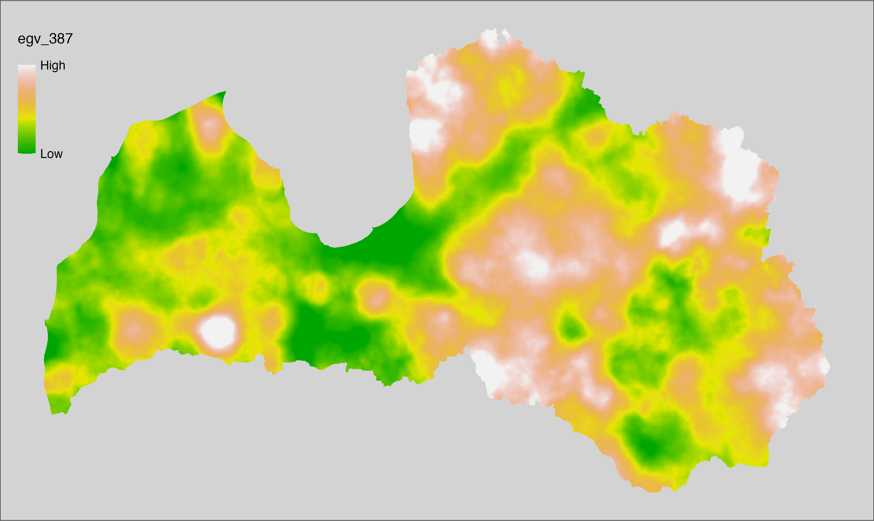
6.388 ForestsTrees_Coniferous_cell
filename: ForestsTrees_Coniferous_cell.tif
layername: egv_388
English name: Fractional cover of Coniferous Forests within the analysis cell (1 ha)
Latvian name: Skujkoku mežu platības īpatsvars analīzes šūnā (1 ha)
Procedure: Most EGVs describing forests are spatially restricted to areas outside of clearcuts and dead stands. This mask is created using a combination of the State Forest Service’s State Forest Registry land category 12 and 14, and The Global Forest Watch pixels classified as lost tree canopy cover since 2020 (raster layer matching input, presence = 1, absence = 0).
To prepare this EGV, stands from the State Forest Service’s State Forest Registry are classified into (in order):
coniferous (see Terminology and acronyms for species codes) if timber volume of those species exceeded 75%;
Boreal deciduous if timber volume of those species exceeded 75%;
temperate deciduous if timber volume of those species exceeded 50%;
mixed otherwise;
then coniferous stands are selected and geometries are
rasterised (presence = 1, NA otherwise). Rasterisation is
performed using the workflow egvtools::polygon2input(), restricting to pixels outside clearcut
mask and covering background with value 0. The resulting layer
is then aggregated to EGV resolution using the workflow egvtools::input2egv(), which
calculates the arithmetic mean to determine the cover fraction. During
aggregation, inverse distance weighted (power = 2) gap filling on the output is
applied to ensure no missing values at the edges. Finally, the layer is
standardised by subtracting the arithmetic mean and dividing by the root mean squared
error.
Code
# libs ----
if(!require(egvtools)) {remotes::install_github("aavotins/egvtools"); require(egvtools)}
if(!require(terra)) {install.packages("terra"); require(terra)}
if(!require(sf)) {install.packages("sf"); require(sf)}
if(!require(tidyverse)) {install.packages("tidyverse"); require(tidyverse)}
if(!require(sfarrow)) {install.packages("sfarrow"); require(sfarrow)}
if(!require(readxl)) {install.packages("readxl"); require(readxl)}
if(!require(raster)) {install.packages("raster"); require(raster)}
if(!require(fasterize)) {install.packages("fasterize"); require(fasterize)}
# templates ----
template100=rast("./Templates/TemplateRasters/LV100m_10km.tif")
template10=rast("./Templates/TemplateRasters/LV10m_10km.tif")
rastrs10=raster(template10)
nulls10=rast("./Templates/TemplateRasters/nulls_LV10m_10km.tif")
nulls100=rast("./Templates/TemplateRasters/nulls_LV100m_10km.tif")
# simple landscape ----
simple_landscape=rast("RasterGrids_10m/2024/Ainava_vienk_mask.tif")
# mvr ----
mvr=st_read_parquet("./Geodata/2024/MVR/nogabali_2024janv.parquet")
mvr$yes=1
# clear cut mask ----
izcirtumi=mvr %>%
filter(zkat %in% c("12","14")) %>%
dplyr::select(yes)
r_izcirtumi_mvr=fasterize(izcirtumi,rastrs10,field="yes")
t_izcirtumi_mvr=rast(r_izcirtumi_mvr)
plot(t_izcirtumi_mvr)
tcl=rast("./Geodata/2024/Trees/GFW/TreeCoverLoss_v1_12.tif")
tcl2=ifel(tcl<20,0,1)
tclX=cover(tcl2,nulls10)
plot(tclX)
clearcut_mask=cover(t_izcirtumi_mvr,tclX,
filename="./RasterGrids_10m/2024/Mask_clearcuts.tif",
overwrite=TRUE)
plot(clearcut_mask)
rm(izcirtumi)
rm(r_izcirtumi_mvr)
rm(t_izcirtumi_mvr)
rm(tcl)
rm(tcl2)
rm(tclX)
# ForestsTrees_Coniferous_cell.tif egv_388 ----
skujkoki=c("1","3","13","14","15","22","23","28") # 8
saurlapji=c("4","6","8","9","19","20","21","32","35","68") # 10
platlapji=c("10","11","12","16","17","18","24","25","26","27","28","29","50",
"61","62","63","64","65","66","67","69") # 21
mvr=mvr %>%
mutate(kraja_skujkoku=ifelse(s10 %in% skujkoki,v10,0)+
ifelse(s11 %in% skujkoki,v11,0)+ifelse(s12 %in% skujkoki,v12,0)+
ifelse(s13 %in% skujkoki,v13,0)+ifelse(s14 %in% skujkoki,v14,0),
kraja_saurlapju=ifelse(s10 %in% saurlapji,v10,0)+
ifelse(s11 %in% saurlapji,v11,0)+ifelse(s12 %in% saurlapji,v12,0)+
ifelse(s13 %in% saurlapji,v13,0)+ifelse(s14 %in% saurlapji,v14,0),
kraja_platlapju=ifelse(s10 %in% platlapji,v10,0)+
ifelse(s11 %in% platlapji,v11,0)+ifelse(s12 %in% platlapji,v12,0)+
ifelse(s13 %in% platlapji,v13,0)+ifelse(s14 %in% platlapji,v14,0)) %>%
mutate(kopeja_kraja=kraja_skujkoku+kraja_platlapju+kraja_saurlapju) %>%
mutate(tips=ifelse(kraja_skujkoku/kopeja_kraja>=0.75,"skujkoku",
ifelse(kraja_saurlapju/kopeja_kraja>=0.75,"saurlapju",
ifelse(kraja_platlapju/kopeja_kraja>0.5,"platlapju",
"jauktu koku"))))
nogabali=mvr %>%
filter(zkat=="10"&tips=="skujkoku")
p2i_rez=egvtools::polygon2input(vector_data = nogabali,
template_path = "./Templates/TemplateRasters/LV10m_10km.tif",
out_path = "./RasterGrids_10m/2024/",
file_name = "ForestsTrees_Coniferous_input.tif",
value_field = "yes",
restrict_to = clearcut_mask,
restrict_values = 0,
prepare=FALSE,
background_raster = "./Templates/TemplateRasters/nulls_LV10m_10km.tif",
plot_result = TRUE)
p2i_rez
i2e_rez=egvtools::input2egv(input=paste0("./RasterGrids_10m/2024/",
"ForestsTrees_Coniferous_input.tif"),
egv_template= "./Templates/TemplateRasters/LV100m_10km.tif",
summary_function = "average",
missing_job = "FillOutput",
outlocation = "./RasterGrids_100m/2024/RAW/",
outfilename = "ForestsTrees_Coniferous_cell.tif",
layername = "egv_388",
idw_weight = 2,
plot_gaps = FALSE,plot_final = TRUE)
i2e_rez
rm(nogabali)
rm(p2i_rez)
rm(i2e_rez)
unlink("./RasterGrids_10m/2024/ForestsTrees_Coniferous_input.tif")
# standardisation ----
if(!require(terra)) {install.packages("terra"); require(terra)}
if(!require(tidyverse)) {install.packages("tidyverse"); require(tidyverse)}
nosaukums="ForestsTrees_Coniferous_cell.tif"
ielasisanas_cels=paste0("./RasterGrids_100m/2024/RAW/",nosaukums)
saglabasanas_cels=paste0("./RasterGrids_100m/2024/Scaled/",nosaukums)
slanis=rast(ielasisanas_cels)
videjais=global(slanis,fun="mean",na.rm=TRUE)
centrets=slanis-videjais[,1]
standartnovirze=terra::global(centrets,fun="rms",na.rm=TRUE)
merogots=centrets/standartnovirze[,1]
writeRaster(merogots,
filename=saglabasanas_cels,
overwrite=TRUE)
6.389 ForestsTrees_Coniferous_r500
filename: ForestsTrees_Coniferous_r500.tif
layername: egv_389
English name: Fractional cover of Coniferous Forests within the 0.5 km landscape
Latvian name: Skujkoku mežu platības īpatsvars 0,5 km ainavā
Procedure: The cover fraction within a radius of 500 m around the analysis grid cell is
calculated as the area-weighted sum of the analysis cells inside the
buffer, using the workflow egvtools::radius_function(). During the calculation of the landscape metric,
inverse distance weighted (power = 2) gap filling on the output is applied
to ensure no missing values at the edges. Then the layer is rewritten to set
its name. Finally, the layer is standardised by subtracting the arithmetic
mean and dividing by the root mean squared error.
Code
# libs ----
if(!require(terra)) {install.packages("terra"); require(terra)}
if(!require(egvtools)) {remotes::install_github("aavotins/egvtools"); require(egvtools)}
# Templates -----
template100=rast("./Templates/TemplateRasters/LV100m_10km.tif")
# radii ----
radius_function(
kvadrati_path = "./Templates/TemplateGrids/tiles/",
radii_path = "./Templates/TemplateGridPoints/tiles/",
tikls100_path = "./Templates/TemplateGrids/tikls100_sauzeme.parquet",
template_path = "./Templates/TemplateRasters/LV100m_10km.tif",
input_layers = c("./RasterGrids_100m/2024/RAW/ForestsTrees_Coniferous_cell.tif"),
layer_prefixes = c("ForestsTrees_Coniferous"),
output_dir = "./RasterGrids_100m/2024/RAW/",
n_workers = 6,
radii = c("r500"),
radius_mode = "sparse",
extract_fun = "mean",
fill_missing = TRUE,
IDW_weight = 2,
future_max_size = 40 * 1024^3)
# ForestsTrees_Coniferous_r500.tif egv_389
slanis=rast("./RasterGrids_100m/2024/RAW/ForestsTrees_Coniferous_r500.tif")
names(slanis)="egv_389"
slanis2=project(slanis,template100)
writeRaster(slanis2,
"./RasterGrids_100m/2024/RAW/ForestsTrees_Coniferous_r500.tif",
overwrite=TRUE)
# standardisation ----
if(!require(terra)) {install.packages("terra"); require(terra)}
if(!require(tidyverse)) {install.packages("tidyverse"); require(tidyverse)}
nosaukums="ForestsTrees_Coniferous_r500.tif"
ielasisanas_cels=paste0("./RasterGrids_100m/2024/RAW/",nosaukums)
saglabasanas_cels=paste0("./RasterGrids_100m/2024/Scaled/",nosaukums)
slanis=rast(ielasisanas_cels)
videjais=global(slanis,fun="mean",na.rm=TRUE)
centrets=slanis-videjais[,1]
standartnovirze=terra::global(centrets,fun="rms",na.rm=TRUE)
merogots=centrets/standartnovirze[,1]
writeRaster(merogots,
filename=saglabasanas_cels,
overwrite=TRUE)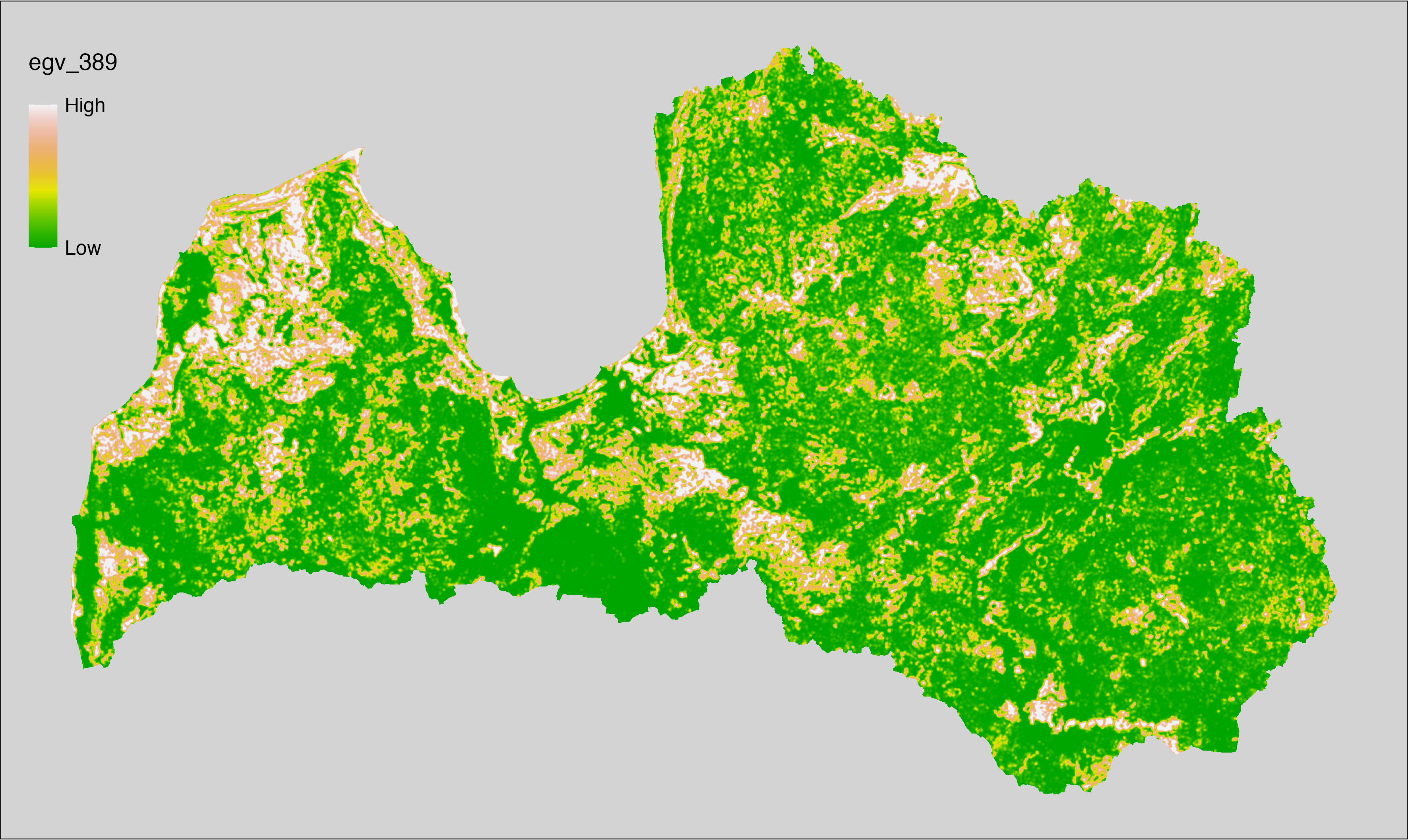
6.390 ForestsTrees_Coniferous_r1250
filename: ForestsTrees_Coniferous_r1250.tif
layername: egv_390
English name: Fractional cover of Coniferous Forests within the 1.25 km landscape
Latvian name: Skujkoku mežu platības īpatsvars 1,25 km ainavā
Procedure: The cover fraction within a radius of 1250 m around the analysis grid cell
is calculated as the area-weighted sum of the analysis cells inside
the buffer, using the workflow egvtools::radius_function(). During the calculation of the landscape
metric, inverse distance weighted (power = 2) gap filling on the output is
applied to ensure no missing values at the edges. Then the layer is
rewritten to set its name. Finally, the layer is standardised by
subtracting the arithmetic mean and dividing by the root mean squared error.
Code
# libs ----
if(!require(terra)) {install.packages("terra"); require(terra)}
if(!require(egvtools)) {remotes::install_github("aavotins/egvtools"); require(egvtools)}
# Templates -----
template100=rast("./Templates/TemplateRasters/LV100m_10km.tif")
# radii ----
radius_function(
kvadrati_path = "./Templates/TemplateGrids/tiles/",
radii_path = "./Templates/TemplateGridPoints/tiles/",
tikls100_path = "./Templates/TemplateGrids/tikls100_sauzeme.parquet",
template_path = "./Templates/TemplateRasters/LV100m_10km.tif",
input_layers = c("./RasterGrids_100m/2024/RAW/ForestsTrees_Coniferous_cell.tif"),
layer_prefixes = c("ForestsTrees_Coniferous"),
output_dir = "./RasterGrids_100m/2024/RAW/",
n_workers = 6,
radii = c("r1250"),
radius_mode = "sparse",
extract_fun = "mean",
fill_missing = TRUE,
IDW_weight = 2,
future_max_size = 40 * 1024^3)
# ForestsTrees_Coniferous_r1250.tif egv_390
slanis=rast("./RasterGrids_100m/2024/RAW/ForestsTrees_Coniferous_r1250.tif")
names(slanis)="egv_390"
slanis2=project(slanis,template100)
writeRaster(slanis2,
"./RasterGrids_100m/2024/RAW/ForestsTrees_Coniferous_r1250.tif",
overwrite=TRUE)
# standardisation ----
if(!require(terra)) {install.packages("terra"); require(terra)}
if(!require(tidyverse)) {install.packages("tidyverse"); require(tidyverse)}
nosaukums="ForestsTrees_Coniferous_r1250.tif"
ielasisanas_cels=paste0("./RasterGrids_100m/2024/RAW/",nosaukums)
saglabasanas_cels=paste0("./RasterGrids_100m/2024/Scaled/",nosaukums)
slanis=rast(ielasisanas_cels)
videjais=global(slanis,fun="mean",na.rm=TRUE)
centrets=slanis-videjais[,1]
standartnovirze=terra::global(centrets,fun="rms",na.rm=TRUE)
merogots=centrets/standartnovirze[,1]
writeRaster(merogots,
filename=saglabasanas_cels,
overwrite=TRUE)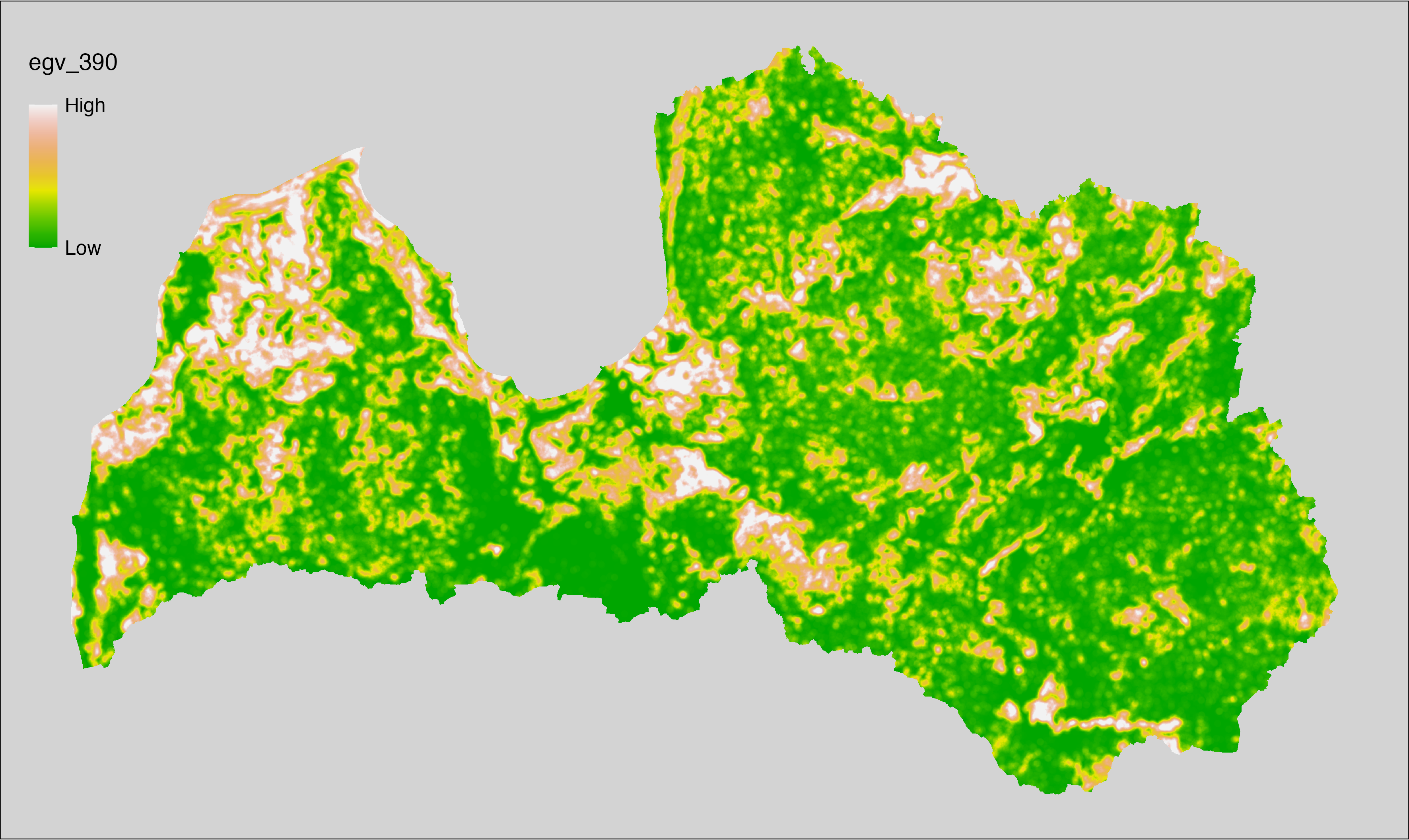
6.391 ForestsTrees_Coniferous_r3000
filename: ForestsTrees_Coniferous_r3000.tif
layername: egv_391
English name: Fractional cover of Coniferous Forests within the 3 km landscape
Latvian name: Skujkoku mežu platības īpatsvars 3 km ainavā
Procedure: The cover fraction within a radius of 3000 m around the analysis grid cell
is calculated as the area-weighted sum of the analysis cells inside
the buffer, using the workflow egvtools::radius_function(). During the calculation of the landscape
metric, inverse distance weighted (power = 2) gap filling on the output is
applied to ensure no missing values at the edges. Then the layer is
rewritten to set its name. Finally, the layer is standardised by
subtracting the arithmetic mean and dividing by the root mean squared error.
Code
# libs ----
if(!require(terra)) {install.packages("terra"); require(terra)}
if(!require(egvtools)) {remotes::install_github("aavotins/egvtools"); require(egvtools)}
# Templates -----
template100=rast("./Templates/TemplateRasters/LV100m_10km.tif")
# radii ----
radius_function(
kvadrati_path = "./Templates/TemplateGrids/tiles/",
radii_path = "./Templates/TemplateGridPoints/tiles/",
tikls100_path = "./Templates/TemplateGrids/tikls100_sauzeme.parquet",
template_path = "./Templates/TemplateRasters/LV100m_10km.tif",
input_layers = c("./RasterGrids_100m/2024/RAW/ForestsTrees_Coniferous_cell.tif"),
layer_prefixes = c("ForestsTrees_Coniferous"),
output_dir = "./RasterGrids_100m/2024/RAW/",
n_workers = 6,
radii = c("r3000"),
radius_mode = "sparse",
extract_fun = "mean",
fill_missing = TRUE,
IDW_weight = 2,
future_max_size = 40 * 1024^3)
# ForestsTrees_Coniferous_r3000.tif egv_391
slanis=rast("./RasterGrids_100m/2024/RAW/ForestsTrees_Coniferous_r3000.tif")
names(slanis)="egv_391"
slanis2=project(slanis,template100)
writeRaster(slanis2,
"./RasterGrids_100m/2024/RAW/ForestsTrees_Coniferous_r3000.tif",
overwrite=TRUE)
# standardisation ----
if(!require(terra)) {install.packages("terra"); require(terra)}
if(!require(tidyverse)) {install.packages("tidyverse"); require(tidyverse)}
nosaukums="ForestsTrees_Coniferous_r3000.tif"
ielasisanas_cels=paste0("./RasterGrids_100m/2024/RAW/",nosaukums)
saglabasanas_cels=paste0("./RasterGrids_100m/2024/Scaled/",nosaukums)
slanis=rast(ielasisanas_cels)
videjais=global(slanis,fun="mean",na.rm=TRUE)
centrets=slanis-videjais[,1]
standartnovirze=terra::global(centrets,fun="rms",na.rm=TRUE)
merogots=centrets/standartnovirze[,1]
writeRaster(merogots,
filename=saglabasanas_cels,
overwrite=TRUE)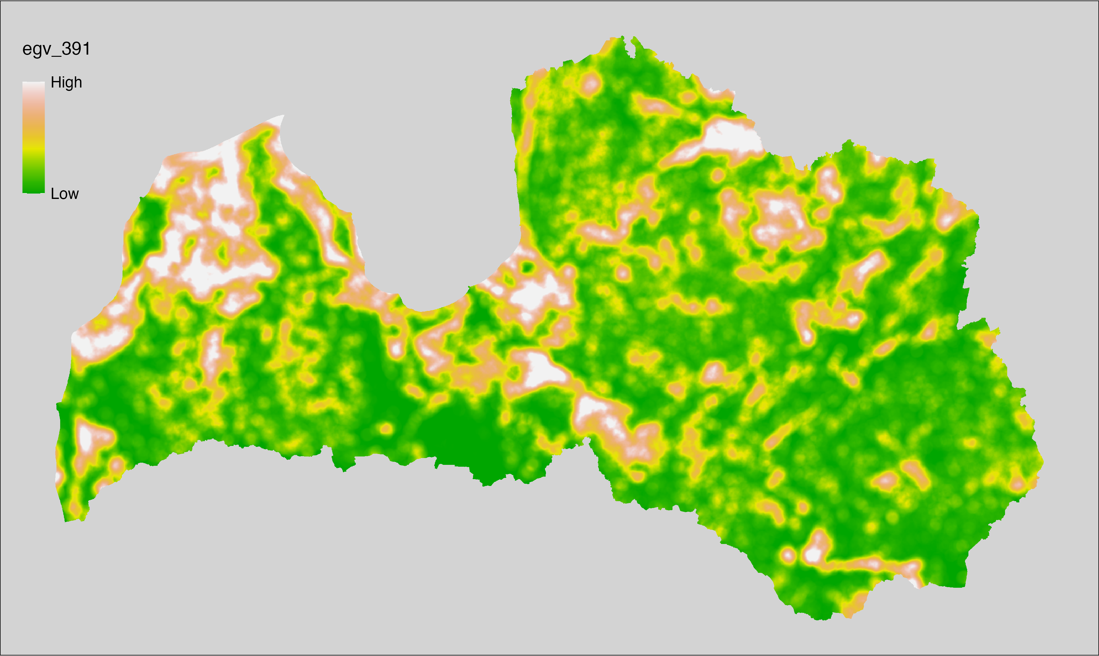
6.392 ForestsTrees_Coniferous_r10000
filename: ForestsTrees_Coniferous_r10000.tif
layername: egv_392
English name: Fractional cover of Coniferous Forests within the 10 km landscape
Latvian name: Skujkoku mežu platības īpatsvars 10 km ainavā
Procedure: The cover fraction within a radius of 10000 m around the analysis grid cell
is calculated as the area-weighted sum of the analysis cells inside
the buffer, using the workflow egvtools::radius_function(). During the calculation of the landscape
metric, inverse distance weighted (power = 2) gap filling on the output is
applied to ensure no missing values at the edges. Then the layer is
rewritten to set its name. Finally, the layer is standardised by
subtracting the arithmetic mean and dividing by the root mean squared error.
Code
# libs ----
if(!require(terra)) {install.packages("terra"); require(terra)}
if(!require(egvtools)) {remotes::install_github("aavotins/egvtools"); require(egvtools)}
# Templates -----
template100=rast("./Templates/TemplateRasters/LV100m_10km.tif")
# radii ----
radius_function(
kvadrati_path = "./Templates/TemplateGrids/tiles/",
radii_path = "./Templates/TemplateGridPoints/tiles/",
tikls100_path = "./Templates/TemplateGrids/tikls100_sauzeme.parquet",
template_path = "./Templates/TemplateRasters/LV100m_10km.tif",
input_layers = c("./RasterGrids_100m/2024/RAW/ForestsTrees_Coniferous_cell.tif"),
layer_prefixes = c("ForestsTrees_Coniferous"),
output_dir = "./RasterGrids_100m/2024/RAW/",
n_workers = 6,
radii = c("r10000"),
radius_mode = "sparse",
extract_fun = "mean",
fill_missing = TRUE,
IDW_weight = 2,
future_max_size = 40 * 1024^3)
# ForestsTrees_Coniferous_r10000.tif egv_392
slanis=rast("./RasterGrids_100m/2024/RAW/ForestsTrees_Coniferous_r10000.tif")
names(slanis)="egv_392"
slanis2=project(slanis,template100)
writeRaster(slanis2,
"./RasterGrids_100m/2024/RAW/ForestsTrees_Coniferous_r10000.tif",
overwrite=TRUE)
# standardisation ----
if(!require(terra)) {install.packages("terra"); require(terra)}
if(!require(tidyverse)) {install.packages("tidyverse"); require(tidyverse)}
nosaukums="ForestsTrees_Coniferous_r10000.tif"
ielasisanas_cels=paste0("./RasterGrids_100m/2024/RAW/",nosaukums)
saglabasanas_cels=paste0("./RasterGrids_100m/2024/Scaled/",nosaukums)
slanis=rast(ielasisanas_cels)
videjais=global(slanis,fun="mean",na.rm=TRUE)
centrets=slanis-videjais[,1]
standartnovirze=terra::global(centrets,fun="rms",na.rm=TRUE)
merogots=centrets/standartnovirze[,1]
writeRaster(merogots,
filename=saglabasanas_cels,
overwrite=TRUE)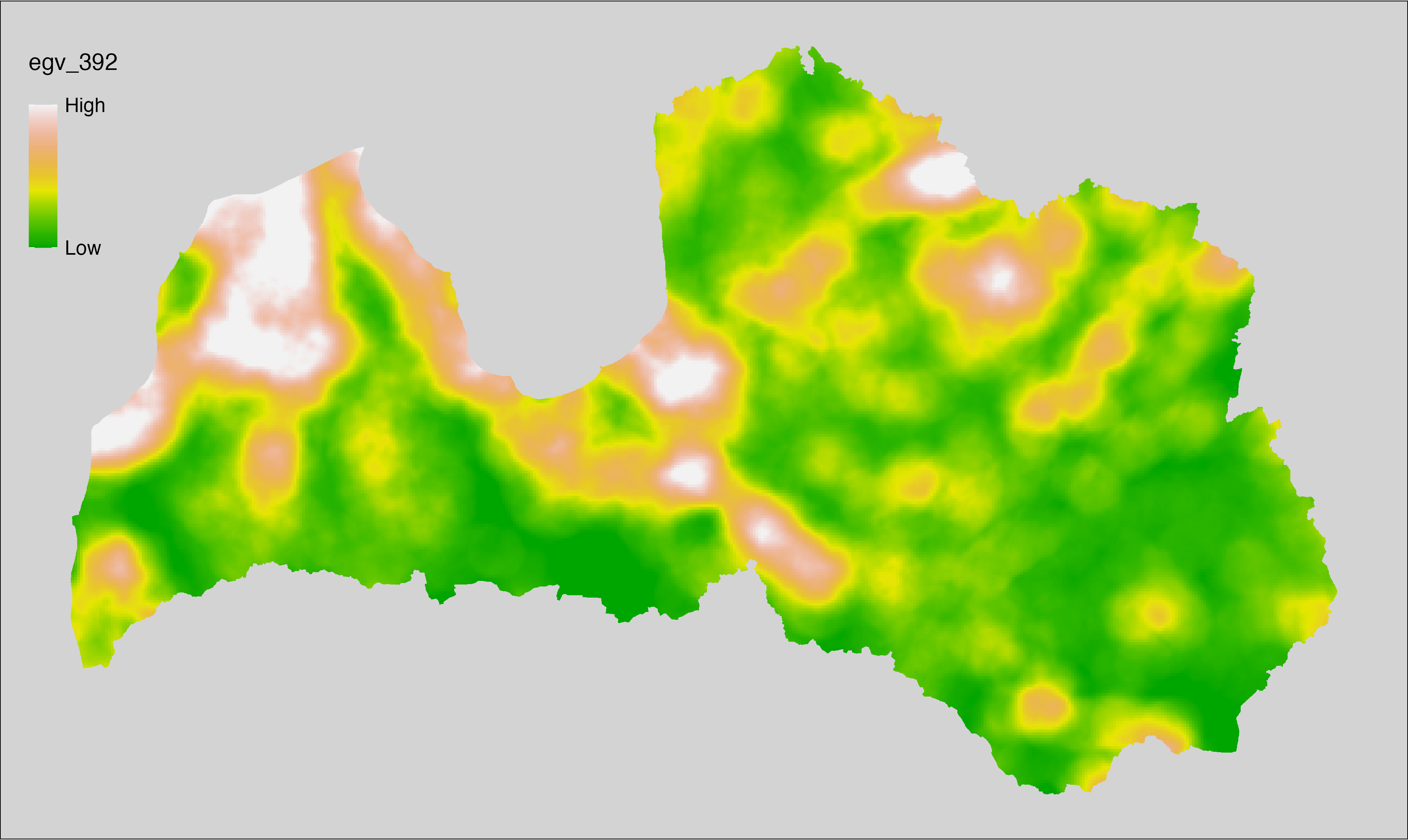
6.393 ForestsTrees_Mixed_cell
filename: ForestsTrees_Mixed_cell.tif
layername: egv_393
English name: Fractional cover of Mixed Forests within the analysis cell (1 ha)
Latvian name: Jauktu koku mežu platības īpatsvars analīzes šūnā (1 ha)
Procedure: Most EGVs describing forests are spatially restricted to areas outside of clearcuts and dead stands. This mask is created using a combination of the State Forest Service’s State Forest Registry land category 12 and 14, and The Global Forest Watch pixels classified as lost tree canopy cover since 2020 (raster layer matching input, presence = 1, absence = 0).
To prepare this EGV, stands from the State Forest Service’s State Forest Registry are classified into (in order):
coniferous (see Terminology and acronyms for species codes) if timber volume of those species exceeded 75%;
Boreal deciduous if timber volume of those species exceeded 75%;
temperate deciduous if timber volume of those species exceeded 50%;
mixed otherwise;
then mixed stands are selected and geometries are
rasterised (presence = 1, NA otherwise). Rasterisation is
performed using the workflow egvtools::polygon2input(), restricting to pixels outside clearcut
mask and covering background with value 0. The resulting layer
is then aggregated to EGV resolution using the workflow egvtools::input2egv(), which
calculates the arithmetic mean to determine the cover fraction. During
aggregation, inverse distance weighted (power = 2) gap filling on the output is
applied to ensure no missing values at the edges. Finally, the layer is
standardised by subtracting the arithmetic mean and dividing by the root mean squared
error.
Code
# libs ----
if(!require(egvtools)) {remotes::install_github("aavotins/egvtools"); require(egvtools)}
if(!require(terra)) {install.packages("terra"); require(terra)}
if(!require(sf)) {install.packages("sf"); require(sf)}
if(!require(tidyverse)) {install.packages("tidyverse"); require(tidyverse)}
if(!require(sfarrow)) {install.packages("sfarrow"); require(sfarrow)}
if(!require(readxl)) {install.packages("readxl"); require(readxl)}
if(!require(raster)) {install.packages("raster"); require(raster)}
if(!require(fasterize)) {install.packages("fasterize"); require(fasterize)}
# templates ----
template100=rast("./Templates/TemplateRasters/LV100m_10km.tif")
template10=rast("./Templates/TemplateRasters/LV10m_10km.tif")
rastrs10=raster(template10)
nulls10=rast("./Templates/TemplateRasters/nulls_LV10m_10km.tif")
nulls100=rast("./Templates/TemplateRasters/nulls_LV100m_10km.tif")
# simple landscape ----
simple_landscape=rast("RasterGrids_10m/2024/Ainava_vienk_mask.tif")
# mvr ----
mvr=st_read_parquet("./Geodata/2024/MVR/nogabali_2024janv.parquet")
mvr$yes=1
# clear cut mask ----
izcirtumi=mvr %>%
filter(zkat %in% c("12","14")) %>%
dplyr::select(yes)
r_izcirtumi_mvr=fasterize(izcirtumi,rastrs10,field="yes")
t_izcirtumi_mvr=rast(r_izcirtumi_mvr)
plot(t_izcirtumi_mvr)
tcl=rast("./Geodata/2024/Trees/GFW/TreeCoverLoss_v1_12.tif")
tcl2=ifel(tcl<20,0,1)
tclX=cover(tcl2,nulls10)
plot(tclX)
clearcut_mask=cover(t_izcirtumi_mvr,tclX,
filename="./RasterGrids_10m/2024/Mask_clearcuts.tif",
overwrite=TRUE)
plot(clearcut_mask)
rm(izcirtumi)
rm(r_izcirtumi_mvr)
rm(t_izcirtumi_mvr)
rm(tcl)
rm(tcl2)
rm(tclX)
# ForestsTrees_Mixed_cell.tif egv_393 ----
skujkoki=c("1","3","13","14","15","22","23","28") # 8
saurlapji=c("4","6","8","9","19","20","21","32","35","68") # 10
platlapji=c("10","11","12","16","17","18","24","25","26","27","28","29","50",
"61","62","63","64","65","66","67","69") # 21
mvr=mvr %>%
mutate(kraja_skujkoku=ifelse(s10 %in% skujkoki,v10,0)+
ifelse(s11 %in% skujkoki,v11,0)+ifelse(s12 %in% skujkoki,v12,0)+
ifelse(s13 %in% skujkoki,v13,0)+ifelse(s14 %in% skujkoki,v14,0),
kraja_saurlapju=ifelse(s10 %in% saurlapji,v10,0)+
ifelse(s11 %in% saurlapji,v11,0)+ifelse(s12 %in% saurlapji,v12,0)+
ifelse(s13 %in% saurlapji,v13,0)+ifelse(s14 %in% saurlapji,v14,0),
kraja_platlapju=ifelse(s10 %in% platlapji,v10,0)+
ifelse(s11 %in% platlapji,v11,0)+ifelse(s12 %in% platlapji,v12,0)+
ifelse(s13 %in% platlapji,v13,0)+ifelse(s14 %in% platlapji,v14,0)) %>%
mutate(kopeja_kraja=kraja_skujkoku+kraja_platlapju+kraja_saurlapju) %>%
mutate(tips=ifelse(kraja_skujkoku/kopeja_kraja>=0.75,"skujkoku",
ifelse(kraja_saurlapju/kopeja_kraja>=0.75,"saurlapju",
ifelse(kraja_platlapju/kopeja_kraja>0.5,"platlapju",
"jauktu koku"))))
nogabali=mvr %>%
filter(zkat=="10"&tips=="jauktu koku")
p2i_rez=egvtools::polygon2input(vector_data = nogabali,
template_path = "./Templates/TemplateRasters/LV10m_10km.tif",
out_path = "./RasterGrids_10m/2024/",
file_name = "ForestsTrees_Mixed_input.tif",
value_field = "yes",
restrict_to = clearcut_mask,
restrict_values = 0,
prepare=FALSE,
background_raster = "./Templates/TemplateRasters/nulls_LV10m_10km.tif",
plot_result = TRUE)
p2i_rez
i2e_rez=egvtools::input2egv(input=paste0("./RasterGrids_10m/2024/",
"ForestsTrees_Mixed_input.tif"),
egv_template= "./Templates/TemplateRasters/LV100m_10km.tif",
summary_function = "average",
missing_job = "FillOutput",
outlocation = "./RasterGrids_100m/2024/RAW/",
outfilename = "ForestsTrees_Mixed_cell.tif",
layername = "egv_393",
idw_weight = 2,
plot_gaps = FALSE,plot_final = TRUE)
i2e_rez
rm(nogabali)
rm(p2i_rez)
rm(i2e_rez)
unlink("./RasterGrids_10m/2024/ForestsTrees_Mixed_input.tif")
# standardisation ----
if(!require(terra)) {install.packages("terra"); require(terra)}
if(!require(tidyverse)) {install.packages("tidyverse"); require(tidyverse)}
nosaukums="ForestsTrees_Mixed_cell.tif"
ielasisanas_cels=paste0("./RasterGrids_100m/2024/RAW/",nosaukums)
saglabasanas_cels=paste0("./RasterGrids_100m/2024/Scaled/",nosaukums)
slanis=rast(ielasisanas_cels)
videjais=global(slanis,fun="mean",na.rm=TRUE)
centrets=slanis-videjais[,1]
standartnovirze=terra::global(centrets,fun="rms",na.rm=TRUE)
merogots=centrets/standartnovirze[,1]
writeRaster(merogots,
filename=saglabasanas_cels,
overwrite=TRUE)
6.394 ForestsTrees_Mixed_r500
filename: ForestsTrees_Mixed_r500.tif
layername: egv_394
English name: Fractional cover of Mixed Forests within the 0.5 km landscape
Latvian name: Jauktu koku mežu platības īpatsvars 0,5 km ainavā
Procedure: The cover fraction within a radius of 500 m around the analysis grid cell is
calculated as the area-weighted sum of the analysis cells inside the
buffer, using the workflow egvtools::radius_function(). During the calculation of the landscape metric,
inverse distance weighted (power = 2) gap filling on the output is applied
to ensure no missing values at the edges. Then the layer is rewritten to set
its name. Finally, the layer is standardised by subtracting the arithmetic
mean and dividing by the root mean squared error.
Code
# libs ----
if(!require(terra)) {install.packages("terra"); require(terra)}
if(!require(egvtools)) {remotes::install_github("aavotins/egvtools"); require(egvtools)}
# Templates -----
template100=rast("./Templates/TemplateRasters/LV100m_10km.tif")
# radii ----
radius_function(
kvadrati_path = "./Templates/TemplateGrids/tiles/",
radii_path = "./Templates/TemplateGridPoints/tiles/",
tikls100_path = "./Templates/TemplateGrids/tikls100_sauzeme.parquet",
template_path = "./Templates/TemplateRasters/LV100m_10km.tif",
input_layers = c("./RasterGrids_100m/2024/RAW/ForestsTrees_Mixed_cell.tif"),
layer_prefixes = c("ForestsTrees_Mixed"),
output_dir = "./RasterGrids_100m/2024/RAW/",
n_workers = 6,
radii = c("r500"),
radius_mode = "sparse",
extract_fun = "mean",
fill_missing = TRUE,
IDW_weight = 2,
future_max_size = 40 * 1024^3)
# ForestsTrees_Mixed_r500.tif egv_394
slanis=rast("./RasterGrids_100m/2024/RAW/ForestsTrees_Mixed_r500.tif")
names(slanis)="egv_394"
slanis2=project(slanis,template100)
writeRaster(slanis2,
"./RasterGrids_100m/2024/RAW/ForestsTrees_Mixed_r500.tif",
overwrite=TRUE)
# standardisation ----
if(!require(terra)) {install.packages("terra"); require(terra)}
if(!require(tidyverse)) {install.packages("tidyverse"); require(tidyverse)}
nosaukums="ForestsTrees_Mixed_r500.tif"
ielasisanas_cels=paste0("./RasterGrids_100m/2024/RAW/",nosaukums)
saglabasanas_cels=paste0("./RasterGrids_100m/2024/Scaled/",nosaukums)
slanis=rast(ielasisanas_cels)
videjais=global(slanis,fun="mean",na.rm=TRUE)
centrets=slanis-videjais[,1]
standartnovirze=terra::global(centrets,fun="rms",na.rm=TRUE)
merogots=centrets/standartnovirze[,1]
writeRaster(merogots,
filename=saglabasanas_cels,
overwrite=TRUE)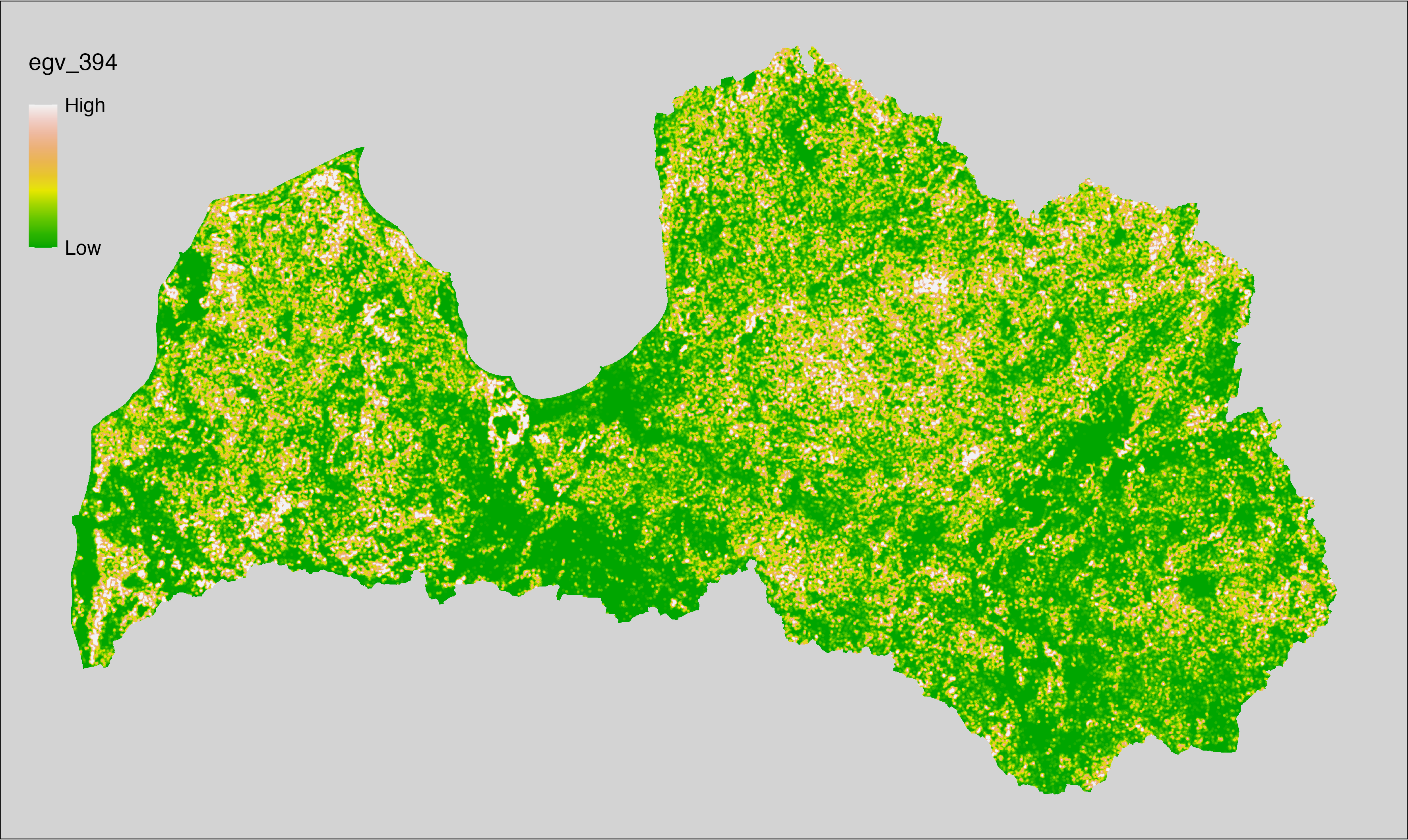
6.395 ForestsTrees_Mixed_r1250
filename: ForestsTrees_Mixed_r1250.tif
layername: egv_395
English name: Fractional cover of Mixed Forests within the 1.25 km landscape
Latvian name: Jauktu koku mežu platības īpatsvars 1,25 km ainavā
Procedure: The cover fraction within a radius of 1250 m around the analysis grid cell
is calculated as the area-weighted sum of the analysis cells inside
the buffer, using the workflow egvtools::radius_function(). During the calculation of the landscape
metric, inverse distance weighted (power = 2) gap filling on the output is
applied to ensure no missing values at the edges. Then the layer is
rewritten to set its name. Finally, the layer is standardised by
subtracting the arithmetic mean and dividing by the root mean squared error.
Code
# libs ----
if(!require(terra)) {install.packages("terra"); require(terra)}
if(!require(egvtools)) {remotes::install_github("aavotins/egvtools"); require(egvtools)}
# Templates -----
template100=rast("./Templates/TemplateRasters/LV100m_10km.tif")
# radii ----
radius_function(
kvadrati_path = "./Templates/TemplateGrids/tiles/",
radii_path = "./Templates/TemplateGridPoints/tiles/",
tikls100_path = "./Templates/TemplateGrids/tikls100_sauzeme.parquet",
template_path = "./Templates/TemplateRasters/LV100m_10km.tif",
input_layers = c("./RasterGrids_100m/2024/RAW/ForestsTrees_Mixed_cell.tif"),
layer_prefixes = c("ForestsTrees_Mixed"),
output_dir = "./RasterGrids_100m/2024/RAW/",
n_workers = 6,
radii = c("r1250"),
radius_mode = "sparse",
extract_fun = "mean",
fill_missing = TRUE,
IDW_weight = 2,
future_max_size = 40 * 1024^3)
# ForestsTrees_Mixed_r1250.tif egv_395
slanis=rast("./RasterGrids_100m/2024/RAW/ForestsTrees_Mixed_r1250.tif")
names(slanis)="egv_395"
slanis2=project(slanis,template100)
writeRaster(slanis2,
"./RasterGrids_100m/2024/RAW/ForestsTrees_Mixed_r1250.tif",
overwrite=TRUE)
# standardisation ----
if(!require(terra)) {install.packages("terra"); require(terra)}
if(!require(tidyverse)) {install.packages("tidyverse"); require(tidyverse)}
nosaukums="ForestsTrees_Mixed_r1250.tif"
ielasisanas_cels=paste0("./RasterGrids_100m/2024/RAW/",nosaukums)
saglabasanas_cels=paste0("./RasterGrids_100m/2024/Scaled/",nosaukums)
slanis=rast(ielasisanas_cels)
videjais=global(slanis,fun="mean",na.rm=TRUE)
centrets=slanis-videjais[,1]
standartnovirze=terra::global(centrets,fun="rms",na.rm=TRUE)
merogots=centrets/standartnovirze[,1]
writeRaster(merogots,
filename=saglabasanas_cels,
overwrite=TRUE)
6.396 ForestsTrees_Mixed_r3000
filename: ForestsTrees_Mixed_r3000.tif
layername: egv_396
English name: Fractional cover of Mixed Forests within the 3 km landscape
Latvian name: Jauktu koku mežu platības īpatsvars 3 km ainavā
Procedure: The cover fraction within a radius of 3000 m around the analysis grid cell
is calculated as the area-weighted sum of the analysis cells inside
the buffer, using the workflow egvtools::radius_function(). During the calculation of the landscape
metric, inverse distance weighted (power = 2) gap filling on the output is
applied to ensure no missing values at the edges. Then the layer is
rewritten to set its name. Finally, the layer is standardised by
subtracting the arithmetic mean and dividing by the root mean squared error.
Code
# libs ----
if(!require(terra)) {install.packages("terra"); require(terra)}
if(!require(egvtools)) {remotes::install_github("aavotins/egvtools"); require(egvtools)}
# Templates -----
template100=rast("./Templates/TemplateRasters/LV100m_10km.tif")
# radii ----
radius_function(
kvadrati_path = "./Templates/TemplateGrids/tiles/",
radii_path = "./Templates/TemplateGridPoints/tiles/",
tikls100_path = "./Templates/TemplateGrids/tikls100_sauzeme.parquet",
template_path = "./Templates/TemplateRasters/LV100m_10km.tif",
input_layers = c("./RasterGrids_100m/2024/RAW/ForestsTrees_Mixed_cell.tif"),
layer_prefixes = c("ForestsTrees_Mixed"),
output_dir = "./RasterGrids_100m/2024/RAW/",
n_workers = 6,
radii = c("r3000"),
radius_mode = "sparse",
extract_fun = "mean",
fill_missing = TRUE,
IDW_weight = 2,
future_max_size = 40 * 1024^3)
# ForestsTrees_Mixed_r3000.tif egv_396
slanis=rast("./RasterGrids_100m/2024/RAW/ForestsTrees_Mixed_r3000.tif")
names(slanis)="egv_396"
slanis2=project(slanis,template100)
writeRaster(slanis2,
"./RasterGrids_100m/2024/RAW/ForestsTrees_Mixed_r3000.tif",
overwrite=TRUE)
# standardisation ----
if(!require(terra)) {install.packages("terra"); require(terra)}
if(!require(tidyverse)) {install.packages("tidyverse"); require(tidyverse)}
nosaukums="ForestsTrees_Mixed_r3000.tif"
ielasisanas_cels=paste0("./RasterGrids_100m/2024/RAW/",nosaukums)
saglabasanas_cels=paste0("./RasterGrids_100m/2024/Scaled/",nosaukums)
slanis=rast(ielasisanas_cels)
videjais=global(slanis,fun="mean",na.rm=TRUE)
centrets=slanis-videjais[,1]
standartnovirze=terra::global(centrets,fun="rms",na.rm=TRUE)
merogots=centrets/standartnovirze[,1]
writeRaster(merogots,
filename=saglabasanas_cels,
overwrite=TRUE)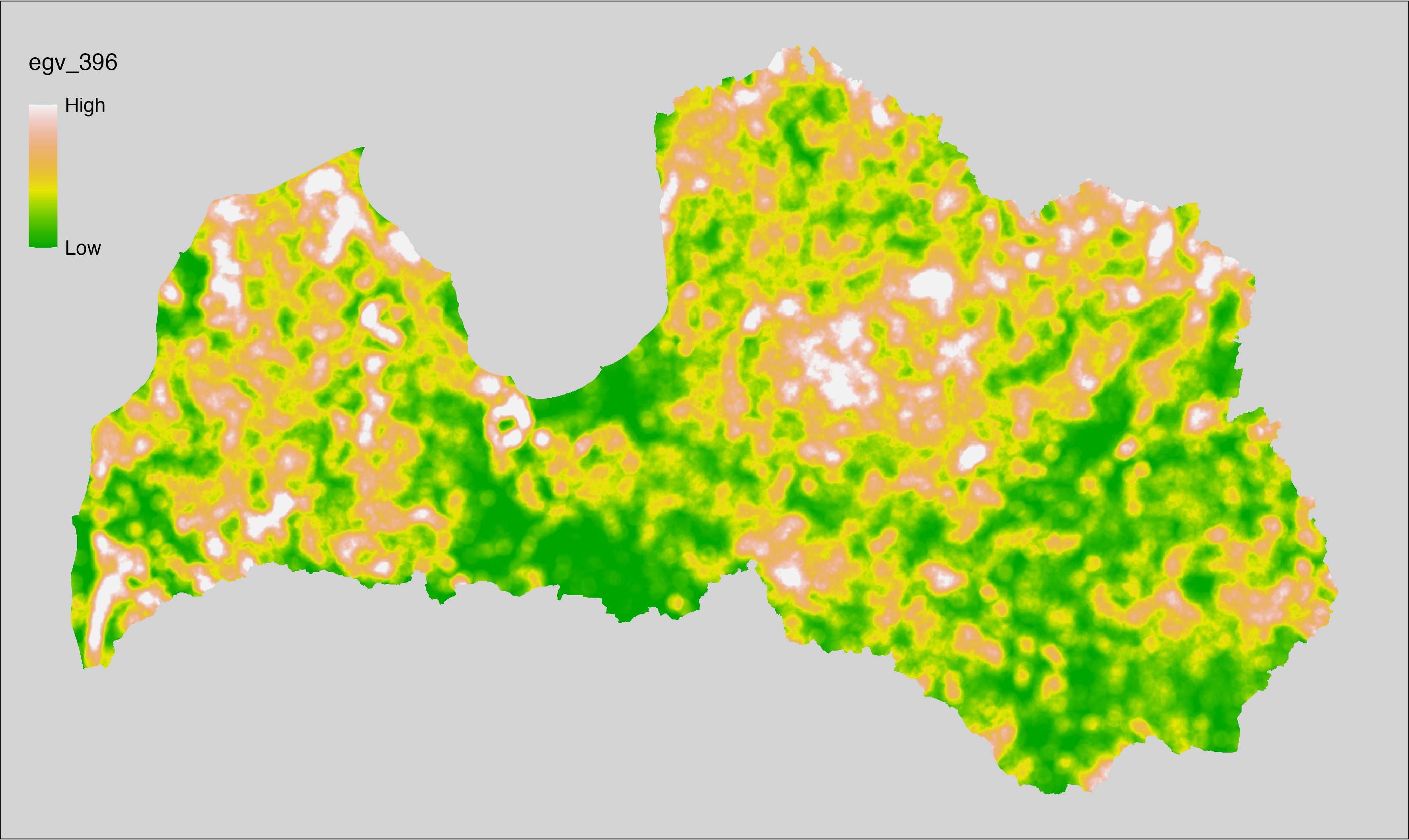
6.397 ForestsTrees_Mixed_r10000
filename: ForestsTrees_Mixed_r10000.tif
layername: egv_397
English name: Fractional cover of Mixed Forests within the 10 km landscape
Latvian name: Jauktu koku mežu platības īpatsvars 10 km ainavā
Procedure: The cover fraction within a radius of 10000 m around the analysis grid cell
is calculated as the area-weighted sum of the analysis cells inside
the buffer, using the workflow egvtools::radius_function(). During the calculation of the landscape
metric, inverse distance weighted (power = 2) gap filling on the output is
applied to ensure no missing values at the edges. Then the layer is
rewritten to set its name. Finally, the layer is standardised by
subtracting the arithmetic mean and dividing by the root mean squared error.
Code
# libs ----
if(!require(terra)) {install.packages("terra"); require(terra)}
if(!require(egvtools)) {remotes::install_github("aavotins/egvtools"); require(egvtools)}
# Templates -----
template100=rast("./Templates/TemplateRasters/LV100m_10km.tif")
# radii ----
radius_function(
kvadrati_path = "./Templates/TemplateGrids/tiles/",
radii_path = "./Templates/TemplateGridPoints/tiles/",
tikls100_path = "./Templates/TemplateGrids/tikls100_sauzeme.parquet",
template_path = "./Templates/TemplateRasters/LV100m_10km.tif",
input_layers = c("./RasterGrids_100m/2024/RAW/ForestsTrees_Mixed_cell.tif"),
layer_prefixes = c("ForestsTrees_Mixed"),
output_dir = "./RasterGrids_100m/2024/RAW/",
n_workers = 6,
radii = c("r10000"),
radius_mode = "sparse",
extract_fun = "mean",
fill_missing = TRUE,
IDW_weight = 2,
future_max_size = 40 * 1024^3)
# ForestsTrees_Mixed_r10000.tif egv_397
slanis=rast("./RasterGrids_100m/2024/RAW/ForestsTrees_Mixed_r10000.tif")
names(slanis)="egv_397"
slanis2=project(slanis,template100)
writeRaster(slanis2,
"./RasterGrids_100m/2024/RAW/ForestsTrees_Mixed_r10000.tif",
overwrite=TRUE)
# standardisation ----
if(!require(terra)) {install.packages("terra"); require(terra)}
if(!require(tidyverse)) {install.packages("tidyverse"); require(tidyverse)}
nosaukums="ForestsTrees_Mixed_r10000.tif"
ielasisanas_cels=paste0("./RasterGrids_100m/2024/RAW/",nosaukums)
saglabasanas_cels=paste0("./RasterGrids_100m/2024/Scaled/",nosaukums)
slanis=rast(ielasisanas_cels)
videjais=global(slanis,fun="mean",na.rm=TRUE)
centrets=slanis-videjais[,1]
standartnovirze=terra::global(centrets,fun="rms",na.rm=TRUE)
merogots=centrets/standartnovirze[,1]
writeRaster(merogots,
filename=saglabasanas_cels,
overwrite=TRUE)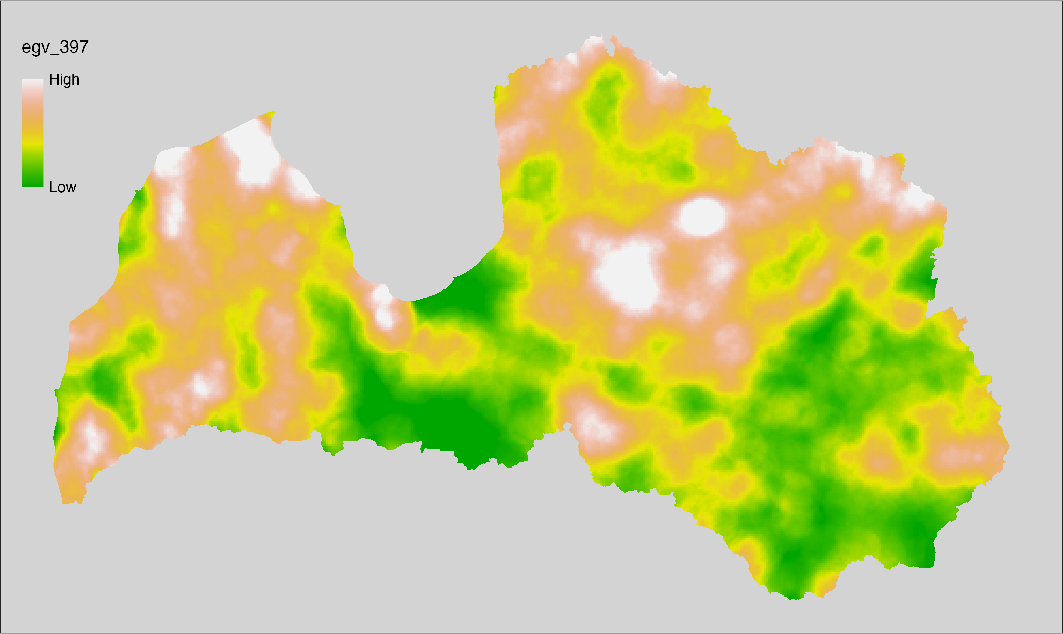
6.398 ForestsTrees_TemperateDeciduous_cell
filename: ForestsTrees_TemperateDeciduous_cell.tif
layername: egv_398
English name: Fractional cover of Temperate Deciduous Forests within the analysis cell (1 ha)
Latvian name: Platlapju mežu platības īpatsvars analīzes šūnā (1 ha)
Procedure: Most EGVs describing forests are spatially restricted to areas outside of clearcuts and dead stands. This mask is created using a combination of the State Forest Service’s State Forest Registry land category 12 and 14, and The Global Forest Watch pixels classified as lost tree canopy cover since 2020 (raster layer matching input, presence = 1, absence = 0).
To prepare this EGV, stands from the State Forest Service’s State Forest Registry are classified into (in order):
coniferous (see Terminology and acronyms for species codes) if timber volume of those species exceeded 75%;
Boreal deciduous if timber volume of those species exceeded 75%;
temperate deciduous if timber volume of those species exceeded 50%;
mixed otherwise;
then temperate deciduous stands are selected and geometries are
rasterised (presence = 1, NA otherwise). Rasterisation is
performed using the workflow egvtools::polygon2input(), restricting to pixels outside clearcut
mask and covering background with value 0. The resulting layer
is then aggregated to EGV resolution using the workflow egvtools::input2egv(), which
calculates the arithmetic mean to determine the cover fraction. During
aggregation, inverse distance weighted (power = 2) gap filling on the output is
applied to ensure no missing values at the edges. Finally, the layer is
standardised by subtracting the arithmetic mean and dividing by the root mean squared
error.
Code
# libs ----
if(!require(egvtools)) {remotes::install_github("aavotins/egvtools"); require(egvtools)}
if(!require(terra)) {install.packages("terra"); require(terra)}
if(!require(sf)) {install.packages("sf"); require(sf)}
if(!require(tidyverse)) {install.packages("tidyverse"); require(tidyverse)}
if(!require(sfarrow)) {install.packages("sfarrow"); require(sfarrow)}
if(!require(readxl)) {install.packages("readxl"); require(readxl)}
if(!require(raster)) {install.packages("raster"); require(raster)}
if(!require(fasterize)) {install.packages("fasterize"); require(fasterize)}
# templates ----
template100=rast("./Templates/TemplateRasters/LV100m_10km.tif")
template10=rast("./Templates/TemplateRasters/LV10m_10km.tif")
rastrs10=raster(template10)
nulls10=rast("./Templates/TemplateRasters/nulls_LV10m_10km.tif")
nulls100=rast("./Templates/TemplateRasters/nulls_LV100m_10km.tif")
# simple landscape ----
simple_landscape=rast("RasterGrids_10m/2024/Ainava_vienk_mask.tif")
# mvr ----
mvr=st_read_parquet("./Geodata/2024/MVR/nogabali_2024janv.parquet")
mvr$yes=1
# clear cut mask ----
izcirtumi=mvr %>%
filter(zkat %in% c("12","14")) %>%
dplyr::select(yes)
r_izcirtumi_mvr=fasterize(izcirtumi,rastrs10,field="yes")
t_izcirtumi_mvr=rast(r_izcirtumi_mvr)
plot(t_izcirtumi_mvr)
tcl=rast("./Geodata/2024/Trees/GFW/TreeCoverLoss_v1_12.tif")
tcl2=ifel(tcl<20,0,1)
tclX=cover(tcl2,nulls10)
plot(tclX)
clearcut_mask=cover(t_izcirtumi_mvr,tclX,
filename="./RasterGrids_10m/2024/Mask_clearcuts.tif",
overwrite=TRUE)
plot(clearcut_mask)
rm(izcirtumi)
rm(r_izcirtumi_mvr)
rm(t_izcirtumi_mvr)
rm(tcl)
rm(tcl2)
rm(tclX)
# ForestsTrees_TemperateDeciduous_cell.tif egv_398 ----
skujkoki=c("1","3","13","14","15","22","23","28") # 8
saurlapji=c("4","6","8","9","19","20","21","32","35","68") # 10
platlapji=c("10","11","12","16","17","18","24","25","26","27","28","29","50",
"61","62","63","64","65","66","67","69") # 21
mvr=mvr %>%
mutate(kraja_skujkoku=ifelse(s10 %in% skujkoki,v10,0)+
ifelse(s11 %in% skujkoki,v11,0)+ifelse(s12 %in% skujkoki,v12,0)+
ifelse(s13 %in% skujkoki,v13,0)+ifelse(s14 %in% skujkoki,v14,0),
kraja_saurlapju=ifelse(s10 %in% saurlapji,v10,0)+
ifelse(s11 %in% saurlapji,v11,0)+ifelse(s12 %in% saurlapji,v12,0)+
ifelse(s13 %in% saurlapji,v13,0)+ifelse(s14 %in% saurlapji,v14,0),
kraja_platlapju=ifelse(s10 %in% platlapji,v10,0)+
ifelse(s11 %in% platlapji,v11,0)+ifelse(s12 %in% platlapji,v12,0)+
ifelse(s13 %in% platlapji,v13,0)+ifelse(s14 %in% platlapji,v14,0)) %>%
mutate(kopeja_kraja=kraja_skujkoku+kraja_platlapju+kraja_saurlapju) %>%
mutate(tips=ifelse(kraja_skujkoku/kopeja_kraja>=0.75,"skujkoku",
ifelse(kraja_saurlapju/kopeja_kraja>=0.75,"saurlapju",
ifelse(kraja_platlapju/kopeja_kraja>0.5,"platlapju",
"jauktu koku"))))
nogabali=mvr %>%
filter(zkat=="10"&tips=="platlapju")
p2i_rez=egvtools::polygon2input(vector_data = nogabali,
template_path = "./Templates/TemplateRasters/LV10m_10km.tif",
out_path = "./RasterGrids_10m/2024/",
file_name = "ForestsTrees_TemperateDeciduous_input.tif",
value_field = "yes",
restrict_to = clearcut_mask,
restrict_values = 0,
prepare=FALSE,
background_raster = "./Templates/TemplateRasters/nulls_LV10m_10km.tif",
plot_result = TRUE)
p2i_rez
i2e_rez=egvtools::input2egv(input=paste0("./RasterGrids_10m/2024/",
"ForestsTrees_TemperateDeciduous_input.tif"),
egv_template= "./Templates/TemplateRasters/LV100m_10km.tif",
summary_function = "average",
missing_job = "FillOutput",
outlocation = "./RasterGrids_100m/2024/RAW/",
outfilename = "ForestsTrees_TemperateDeciduous_cell.tif",
layername = "egv_398",
idw_weight = 2,
plot_gaps = FALSE,plot_final = TRUE)
i2e_rez
rm(nogabali)
rm(p2i_rez)
rm(i2e_rez)
unlink("./RasterGrids_10m/2024/ForestsTrees_TemperateDeciduous_input.tif")
# standardisation ----
if(!require(terra)) {install.packages("terra"); require(terra)}
if(!require(tidyverse)) {install.packages("tidyverse"); require(tidyverse)}
nosaukums="ForestsTrees_TemperateDeciduous_cell.tif"
ielasisanas_cels=paste0("./RasterGrids_100m/2024/RAW/",nosaukums)
saglabasanas_cels=paste0("./RasterGrids_100m/2024/Scaled/",nosaukums)
slanis=rast(ielasisanas_cels)
videjais=global(slanis,fun="mean",na.rm=TRUE)
centrets=slanis-videjais[,1]
standartnovirze=terra::global(centrets,fun="rms",na.rm=TRUE)
merogots=centrets/standartnovirze[,1]
writeRaster(merogots,
filename=saglabasanas_cels,
overwrite=TRUE)
6.399 ForestsTrees_TemperateDeciduous_r500
filename: ForestsTrees_TemperateDeciduous_r500.tif
layername: egv_399
English name: Fractional cover of Temperate Deciduous Forests within the 0.5 km landscape
Latvian name: Platlapju mežu platības īpatsvars 0,5 km ainavā
Procedure: The cover fraction within a radius of 500 m around the analysis grid cell is
calculated as the area-weighted sum of the analysis cells inside the
buffer, using the workflow egvtools::radius_function(). During the calculation of the landscape metric,
inverse distance weighted (power = 2) gap filling on the output is applied
to ensure no missing values at the edges. Then the layer is rewritten to set
its name. Finally, the layer is standardised by subtracting the arithmetic
mean and dividing by the root mean squared error.
Code
# libs ----
if(!require(terra)) {install.packages("terra"); require(terra)}
if(!require(egvtools)) {remotes::install_github("aavotins/egvtools"); require(egvtools)}
# Templates -----
template100=rast("./Templates/TemplateRasters/LV100m_10km.tif")
# radii ----
radius_function(
kvadrati_path = "./Templates/TemplateGrids/tiles/",
radii_path = "./Templates/TemplateGridPoints/tiles/",
tikls100_path = "./Templates/TemplateGrids/tikls100_sauzeme.parquet",
template_path = "./Templates/TemplateRasters/LV100m_10km.tif",
input_layers = c("./RasterGrids_100m/2024/RAW/ForestsTrees_TemperateDeciduous_cell.tif"),
layer_prefixes = c("ForestsTrees_TemperateDeciduous"),
output_dir = "./RasterGrids_100m/2024/RAW/",
n_workers = 6,
radii = c("r500"),
radius_mode = "sparse",
extract_fun = "mean",
fill_missing = TRUE,
IDW_weight = 2,
future_max_size = 40 * 1024^3)
# ForestsTrees_TemperateDeciduous_r500.tif egv_399
slanis=rast("./RasterGrids_100m/2024/RAW/ForestsTrees_TemperateDeciduous_r500.tif")
names(slanis)="egv_399"
slanis2=project(slanis,template100)
writeRaster(slanis2,
"./RasterGrids_100m/2024/RAW/ForestsTrees_TemperateDeciduous_r500.tif",
overwrite=TRUE)
# standardisation ----
if(!require(terra)) {install.packages("terra"); require(terra)}
if(!require(tidyverse)) {install.packages("tidyverse"); require(tidyverse)}
nosaukums="ForestsTrees_TemperateDeciduous_r500.tif"
ielasisanas_cels=paste0("./RasterGrids_100m/2024/RAW/",nosaukums)
saglabasanas_cels=paste0("./RasterGrids_100m/2024/Scaled/",nosaukums)
slanis=rast(ielasisanas_cels)
videjais=global(slanis,fun="mean",na.rm=TRUE)
centrets=slanis-videjais[,1]
standartnovirze=terra::global(centrets,fun="rms",na.rm=TRUE)
merogots=centrets/standartnovirze[,1]
writeRaster(merogots,
filename=saglabasanas_cels,
overwrite=TRUE)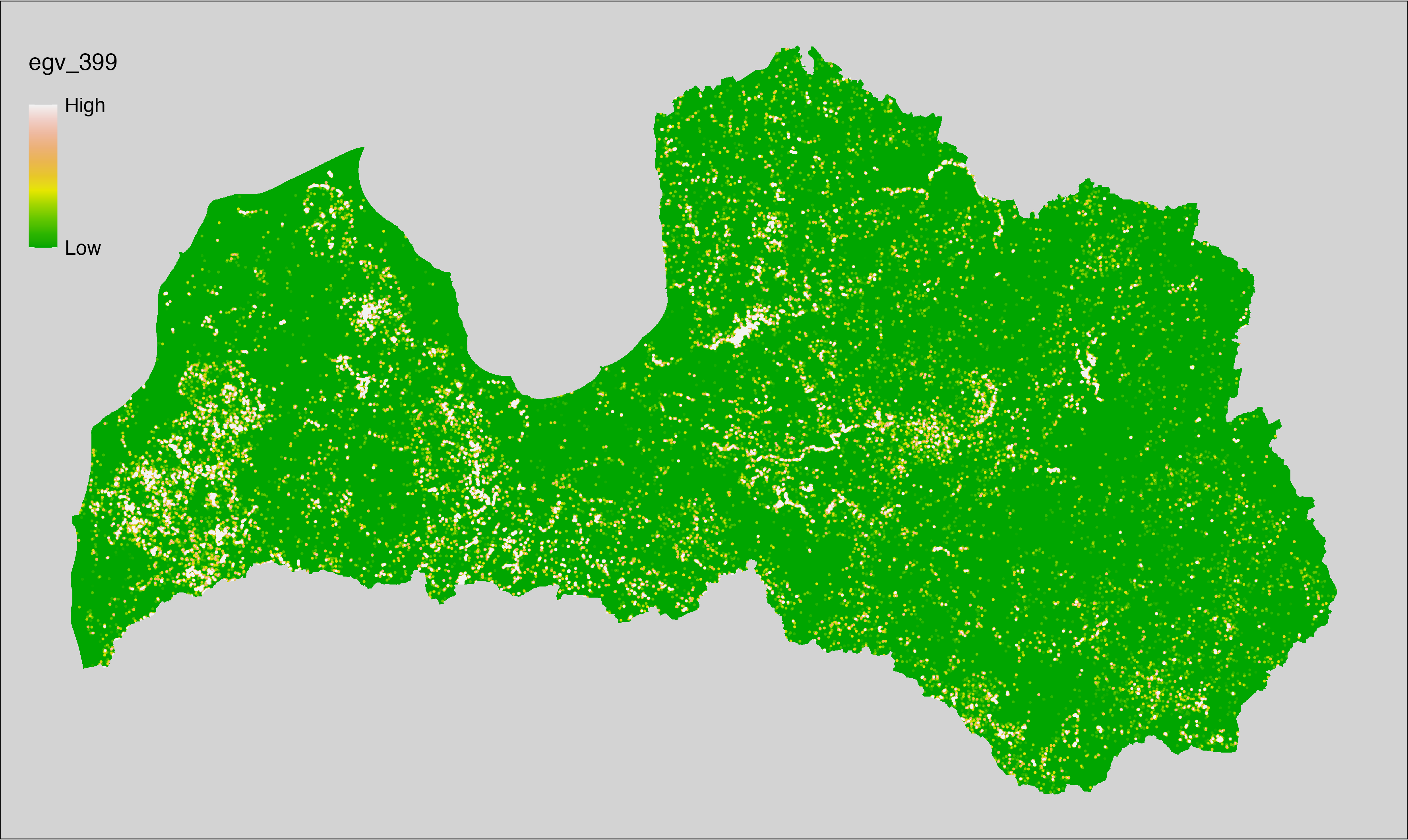
6.400 ForestsTrees_TemperateDeciduous_r1250
filename: ForestsTrees_TemperateDeciduous_r1250.tif
layername: egv_400
English name: Fractional cover of Temperate Deciduous Forests within the 1.25 km landscape
Latvian name: Platlapju mežu platības īpatsvars 1,25 km ainavā
Procedure: The cover fraction within a radius of 1250 m around the analysis grid cell
is calculated as the area-weighted sum of the analysis cells inside
the buffer, using the workflow egvtools::radius_function(). During the calculation of the landscape
metric, inverse distance weighted (power = 2) gap filling on the output is
applied to ensure no missing values at the edges. Then the layer is
rewritten to set its name. Finally, the layer is standardised by
subtracting the arithmetic mean and dividing by the root mean squared error.
Code
# libs ----
if(!require(terra)) {install.packages("terra"); require(terra)}
if(!require(egvtools)) {remotes::install_github("aavotins/egvtools"); require(egvtools)}
# Templates -----
template100=rast("./Templates/TemplateRasters/LV100m_10km.tif")
# radii ----
radius_function(
kvadrati_path = "./Templates/TemplateGrids/tiles/",
radii_path = "./Templates/TemplateGridPoints/tiles/",
tikls100_path = "./Templates/TemplateGrids/tikls100_sauzeme.parquet",
template_path = "./Templates/TemplateRasters/LV100m_10km.tif",
input_layers = c("./RasterGrids_100m/2024/RAW/ForestsTrees_TemperateDeciduous_cell.tif"),
layer_prefixes = c("ForestsTrees_TemperateDeciduous"),
output_dir = "./RasterGrids_100m/2024/RAW/",
n_workers = 6,
radii = c("r1250"),
radius_mode = "sparse",
extract_fun = "mean",
fill_missing = TRUE,
IDW_weight = 2,
future_max_size = 40 * 1024^3)
# ForestsTrees_TemperateDeciduous_r1250.tif egv_400
slanis=rast("./RasterGrids_100m/2024/RAW/ForestsTrees_TemperateDeciduous_r1250.tif")
names(slanis)="egv_400"
slanis2=project(slanis,template100)
writeRaster(slanis2,
"./RasterGrids_100m/2024/RAW/ForestsTrees_TemperateDeciduous_r1250.tif",
overwrite=TRUE)
# standardisation ----
if(!require(terra)) {install.packages("terra"); require(terra)}
if(!require(tidyverse)) {install.packages("tidyverse"); require(tidyverse)}
nosaukums="ForestsTrees_TemperateDeciduous_r1250.tif"
ielasisanas_cels=paste0("./RasterGrids_100m/2024/RAW/",nosaukums)
saglabasanas_cels=paste0("./RasterGrids_100m/2024/Scaled/",nosaukums)
slanis=rast(ielasisanas_cels)
videjais=global(slanis,fun="mean",na.rm=TRUE)
centrets=slanis-videjais[,1]
standartnovirze=terra::global(centrets,fun="rms",na.rm=TRUE)
merogots=centrets/standartnovirze[,1]
writeRaster(merogots,
filename=saglabasanas_cels,
overwrite=TRUE)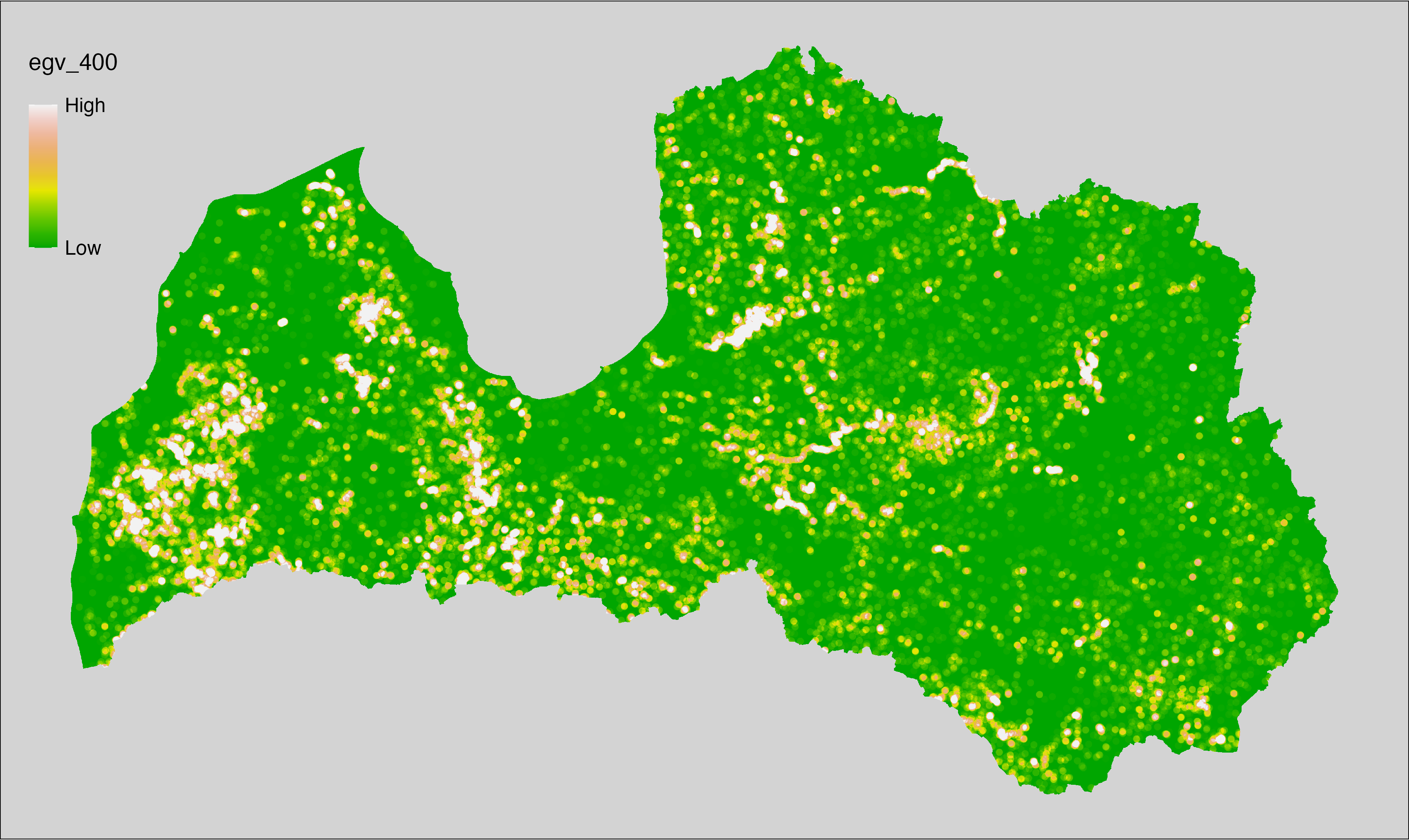
6.401 ForestsTrees_TemperateDeciduous_r3000
filename: ForestsTrees_TemperateDeciduous_r3000.tif
layername: egv_401
English name: Fractional cover of Temperate Deciduous Forests within the 3 km landscape
Latvian name: Platlapju mežu platības īpatsvars 3 km ainavā
Procedure: The cover fraction within a radius of 3000 m around the analysis grid cell
is calculated as the area-weighted sum of the analysis cells inside
the buffer, using the workflow egvtools::radius_function(). During the calculation of the landscape
metric, inverse distance weighted (power = 2) gap filling on the output is
applied to ensure no missing values at the edges. Then the layer is
rewritten to set its name. Finally, the layer is standardised by
subtracting the arithmetic mean and dividing by the root mean squared error.
Code
# libs ----
if(!require(terra)) {install.packages("terra"); require(terra)}
if(!require(egvtools)) {remotes::install_github("aavotins/egvtools"); require(egvtools)}
# Templates -----
template100=rast("./Templates/TemplateRasters/LV100m_10km.tif")
# radii ----
radius_function(
kvadrati_path = "./Templates/TemplateGrids/tiles/",
radii_path = "./Templates/TemplateGridPoints/tiles/",
tikls100_path = "./Templates/TemplateGrids/tikls100_sauzeme.parquet",
template_path = "./Templates/TemplateRasters/LV100m_10km.tif",
input_layers = c("./RasterGrids_100m/2024/RAW/ForestsTrees_TemperateDeciduous_cell.tif"),
layer_prefixes = c("ForestsTrees_TemperateDeciduous"),
output_dir = "./RasterGrids_100m/2024/RAW/",
n_workers = 6,
radii = c("r3000"),
radius_mode = "sparse",
extract_fun = "mean",
fill_missing = TRUE,
IDW_weight = 2,
future_max_size = 40 * 1024^3)
# ForestsTrees_TemperateDeciduous_r3000.tif egv_401
slanis=rast("./RasterGrids_100m/2024/RAW/ForestsTrees_TemperateDeciduous_r3000.tif")
names(slanis)="egv_401"
slanis2=project(slanis,template100)
writeRaster(slanis2,
"./RasterGrids_100m/2024/RAW/ForestsTrees_TemperateDeciduous_r3000.tif",
overwrite=TRUE)
# standardisation ----
if(!require(terra)) {install.packages("terra"); require(terra)}
if(!require(tidyverse)) {install.packages("tidyverse"); require(tidyverse)}
nosaukums="ForestsTrees_TemperateDeciduous_r3000.tif"
ielasisanas_cels=paste0("./RasterGrids_100m/2024/RAW/",nosaukums)
saglabasanas_cels=paste0("./RasterGrids_100m/2024/Scaled/",nosaukums)
slanis=rast(ielasisanas_cels)
videjais=global(slanis,fun="mean",na.rm=TRUE)
centrets=slanis-videjais[,1]
standartnovirze=terra::global(centrets,fun="rms",na.rm=TRUE)
merogots=centrets/standartnovirze[,1]
writeRaster(merogots,
filename=saglabasanas_cels,
overwrite=TRUE)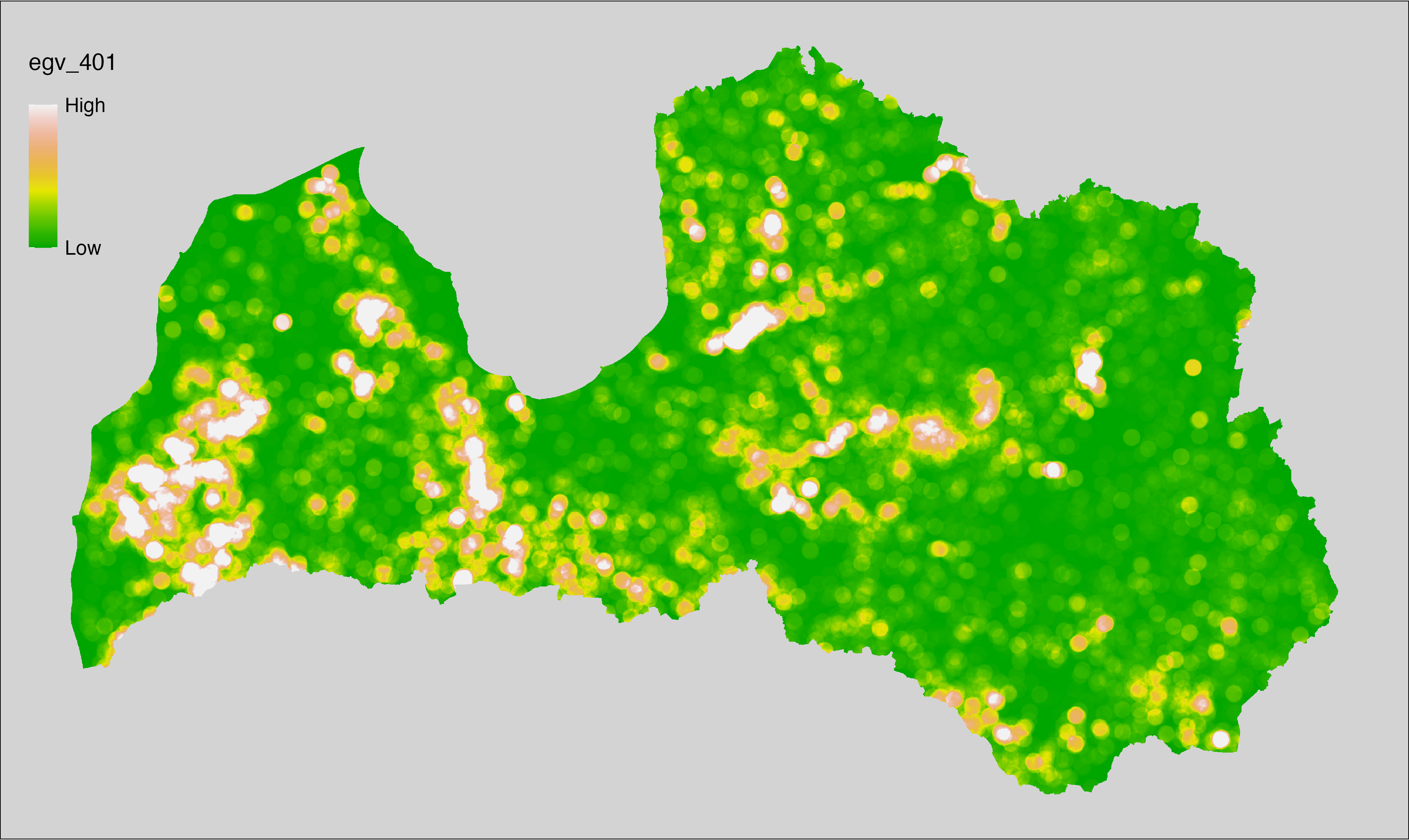
6.402 ForestsTrees_TemperateDeciduous_r10000
filename: ForestsTrees_TemperateDeciduous_r10000.tif
layername: egv_402
English name: Fractional cover of Temperate Deciduous Forests within the 10 km landscape
Latvian name: Platlapju mežu platības īpatsvars 10 km ainavā
Procedure: The cover fraction within a radius of 10000 m around the analysis grid cell
is calculated as the area-weighted sum of the analysis cells inside
the buffer, using the workflow egvtools::radius_function(). During the calculation of the landscape
metric, inverse distance weighted (power = 2) gap filling on the output is
applied to ensure no missing values at the edges. Then the layer is
rewritten to set its name. Finally, the layer is standardised by
subtracting the arithmetic mean and dividing by the root mean squared error.
Code
# libs ----
if(!require(terra)) {install.packages("terra"); require(terra)}
if(!require(egvtools)) {remotes::install_github("aavotins/egvtools"); require(egvtools)}
# Templates -----
template100=rast("./Templates/TemplateRasters/LV100m_10km.tif")
# radii ----
radius_function(
kvadrati_path = "./Templates/TemplateGrids/tiles/",
radii_path = "./Templates/TemplateGridPoints/tiles/",
tikls100_path = "./Templates/TemplateGrids/tikls100_sauzeme.parquet",
template_path = "./Templates/TemplateRasters/LV100m_10km.tif",
input_layers = c("./RasterGrids_100m/2024/RAW/ForestsTrees_TemperateDeciduous_cell.tif"),
layer_prefixes = c("ForestsTrees_TemperateDeciduous"),
output_dir = "./RasterGrids_100m/2024/RAW/",
n_workers = 6,
radii = c("r10000"),
radius_mode = "sparse",
extract_fun = "mean",
fill_missing = TRUE,
IDW_weight = 2,
future_max_size = 40 * 1024^3)
# ForestsTrees_TemperateDeciduous_r10000.tif egv_402
slanis=rast("./RasterGrids_100m/2024/RAW/ForestsTrees_TemperateDeciduous_r10000.tif")
names(slanis)="egv_402"
slanis2=project(slanis,template100)
writeRaster(slanis2,
"./RasterGrids_100m/2024/RAW/ForestsTrees_TemperateDeciduous_r10000.tif",
overwrite=TRUE)
# standardisation ----
if(!require(terra)) {install.packages("terra"); require(terra)}
if(!require(tidyverse)) {install.packages("tidyverse"); require(tidyverse)}
nosaukums="ForestsTrees_TemperateDeciduous_r10000.tif"
ielasisanas_cels=paste0("./RasterGrids_100m/2024/RAW/",nosaukums)
saglabasanas_cels=paste0("./RasterGrids_100m/2024/Scaled/",nosaukums)
slanis=rast(ielasisanas_cels)
videjais=global(slanis,fun="mean",na.rm=TRUE)
centrets=slanis-videjais[,1]
standartnovirze=terra::global(centrets,fun="rms",na.rm=TRUE)
merogots=centrets/standartnovirze[,1]
writeRaster(merogots,
filename=saglabasanas_cels,
overwrite=TRUE)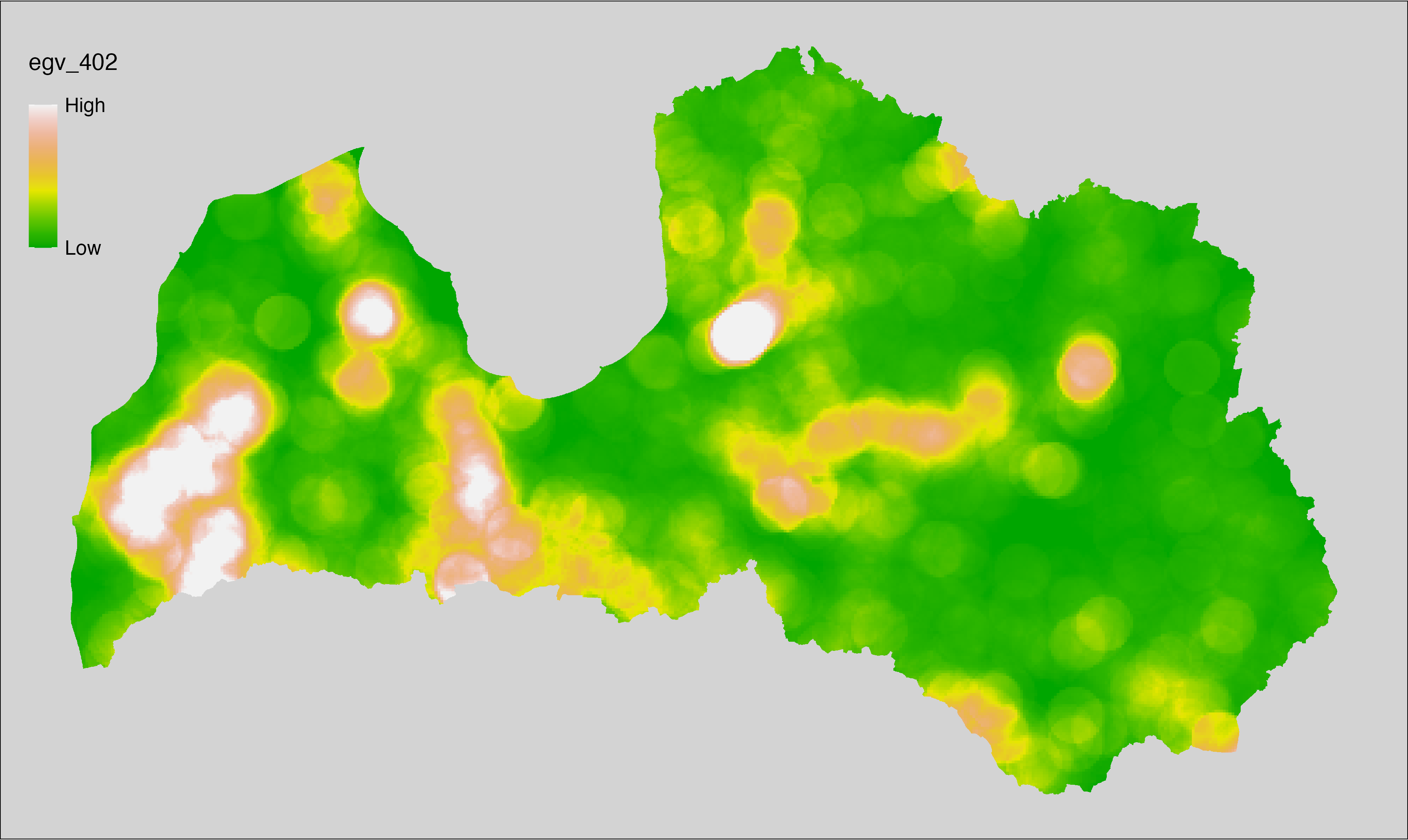
6.403 General_AllotmentGardens_cell
filename: General_AllotmentGardens_cell.tif
layername: egv_403
English name: Fractional cover of Allotment gardens within the analysis cell (1 ha)
Latvian name: Vasarnīcu kompleksu platības īpatsvars analīzes šūnā (1 ha)
Procedure: First, the allotment gardens and farmsteads from the Landscape
classification are selected (value 410 is reclassified to value 1;
all others are set to 0). The resulting layer
is then aggregated to EGV resolution using the workflow egvtools::input2egv(), which
calculates the arithmetic mean to determine the cover fraction. During
aggregation, inverse distance weighted (power = 2) gap filling on the output is
applied to ensure no missing values at the edges. Finally, the layer is
standardised by subtracting the arithmetic mean and dividing by the root mean squared
error.
Code
# libs ----
if(!require(egvtools)) {remotes::install_github("aavotins/egvtools"); require(egvtools)}
if(!require(terra)) {install.packages("terra"); require(terra)}
if(!require(sf)) {install.packages("sf"); require(sf)}
if(!require(tidyverse)) {install.packages("tidyverse"); require(tidyverse)}
if(!require(sfarrow)) {install.packages("sfarrow"); require(sfarrow)}
if(!require(readxl)) {install.packages("readxl"); require(readxl)}
if(!require(raster)) {install.packages("raster"); require(raster)}
if(!require(fasterize)) {install.packages("fasterize"); require(fasterize)}
# templates ----
template100=rast("./Templates/TemplateRasters/LV100m_10km.tif")
template10=rast("./Templates/TemplateRasters/LV10m_10km.tif")
rastrs10=raster(template10)
nulls10=rast("./Templates/TemplateRasters/nulls_LV10m_10km.tif")
nulls100=rast("./Templates/TemplateRasters/nulls_LV100m_10km.tif")
# simple landscape ----
simple_landscape=rast("RasterGrids_10m/2024/Ainava_vienk_mask.tif")
# General_AllotmentGardens_cell.tif egv_403 ----
allotmentgardens=ifel(simple_landscape==410,1,0)
i2e_rez=egvtools::input2egv(input=allotmentgardens,
egv_template= "./Templates/TemplateRasters/LV100m_10km.tif",
summary_function = "average",
missing_job = "FillOutput",
outlocation = "./RasterGrids_100m/2024/RAW/",
outfilename = "General_AllotmentGardens_cell.tif",
layername = "egv_403",
idw_weight = 2,
plot_gaps = FALSE,plot_final = TRUE)
i2e_rez
rm(allotmentgardens)
rm(i2e_rez)
# standardisation ----
if(!require(terra)) {install.packages("terra"); require(terra)}
if(!require(tidyverse)) {install.packages("tidyverse"); require(tidyverse)}
nosaukums="General_AllotmentGardens_cell.tif"
ielasisanas_cels=paste0("./RasterGrids_100m/2024/RAW/",nosaukums)
saglabasanas_cels=paste0("./RasterGrids_100m/2024/Scaled/",nosaukums)
slanis=rast(ielasisanas_cels)
videjais=global(slanis,fun="mean",na.rm=TRUE)
centrets=slanis-videjais[,1]
standartnovirze=terra::global(centrets,fun="rms",na.rm=TRUE)
merogots=centrets/standartnovirze[,1]
writeRaster(merogots,
filename=saglabasanas_cels,
overwrite=TRUE)
6.404 General_AllotmentGardens_r500
filename: General_AllotmentGardens_r500.tif
layername: egv_404
English name: Fractional cover of Allotment gardens within the 0.5 km landscape
Latvian name: Vasarnīcu kompleksu platības īpatsvars 0,5 km ainavā
Procedure: The cover fraction within a radius of 500 m around the analysis grid cell is
calculated as the area-weighted sum of the analysis cells inside the
buffer, using the workflow egvtools::radius_function(). During the calculation of the landscape metric,
inverse distance weighted (power = 2) gap filling on the output is applied
to ensure no missing values at the edges. Then the layer is rewritten to set
its name. Finally, the layer is standardised by subtracting the arithmetic
mean and dividing by the root mean squared error.
Code
# libs ----
if(!require(terra)) {install.packages("terra"); require(terra)}
if(!require(egvtools)) {remotes::install_github("aavotins/egvtools"); require(egvtools)}
# Templates -----
template100=rast("./Templates/TemplateRasters/LV100m_10km.tif")
# radii ----
radius_function(
kvadrati_path = "./Templates/TemplateGrids/tiles/",
radii_path = "./Templates/TemplateGridPoints/tiles/",
tikls100_path = "./Templates/TemplateGrids/tikls100_sauzeme.parquet",
template_path = "./Templates/TemplateRasters/LV100m_10km.tif",
input_layers = c("./RasterGrids_100m/2024/RAW/General_AllotmentGardens_cell.tif"),
layer_prefixes = c("General_AllotmentGardens"),
output_dir = "./RasterGrids_100m/2024/RAW/",
n_workers = 6,
radii = c("r500"),
radius_mode = "sparse",
extract_fun = "mean",
fill_missing = TRUE,
IDW_weight = 2,
future_max_size = 40 * 1024^3)
# General_AllotmentGardens_r500.tif egv_404
slanis=rast("./RasterGrids_100m/2024/RAW/General_AllotmentGardens_r500.tif")
names(slanis)="egv_404"
slanis2=project(slanis,template100)
writeRaster(slanis2,
"./RasterGrids_100m/2024/RAW/General_AllotmentGardens_r500.tif",
overwrite=TRUE)
# standardisation ----
if(!require(terra)) {install.packages("terra"); require(terra)}
if(!require(tidyverse)) {install.packages("tidyverse"); require(tidyverse)}
nosaukums="General_AllotmentGardens_r500.tif"
ielasisanas_cels=paste0("./RasterGrids_100m/2024/RAW/",nosaukums)
saglabasanas_cels=paste0("./RasterGrids_100m/2024/Scaled/",nosaukums)
slanis=rast(ielasisanas_cels)
videjais=global(slanis,fun="mean",na.rm=TRUE)
centrets=slanis-videjais[,1]
standartnovirze=terra::global(centrets,fun="rms",na.rm=TRUE)
merogots=centrets/standartnovirze[,1]
writeRaster(merogots,
filename=saglabasanas_cels,
overwrite=TRUE)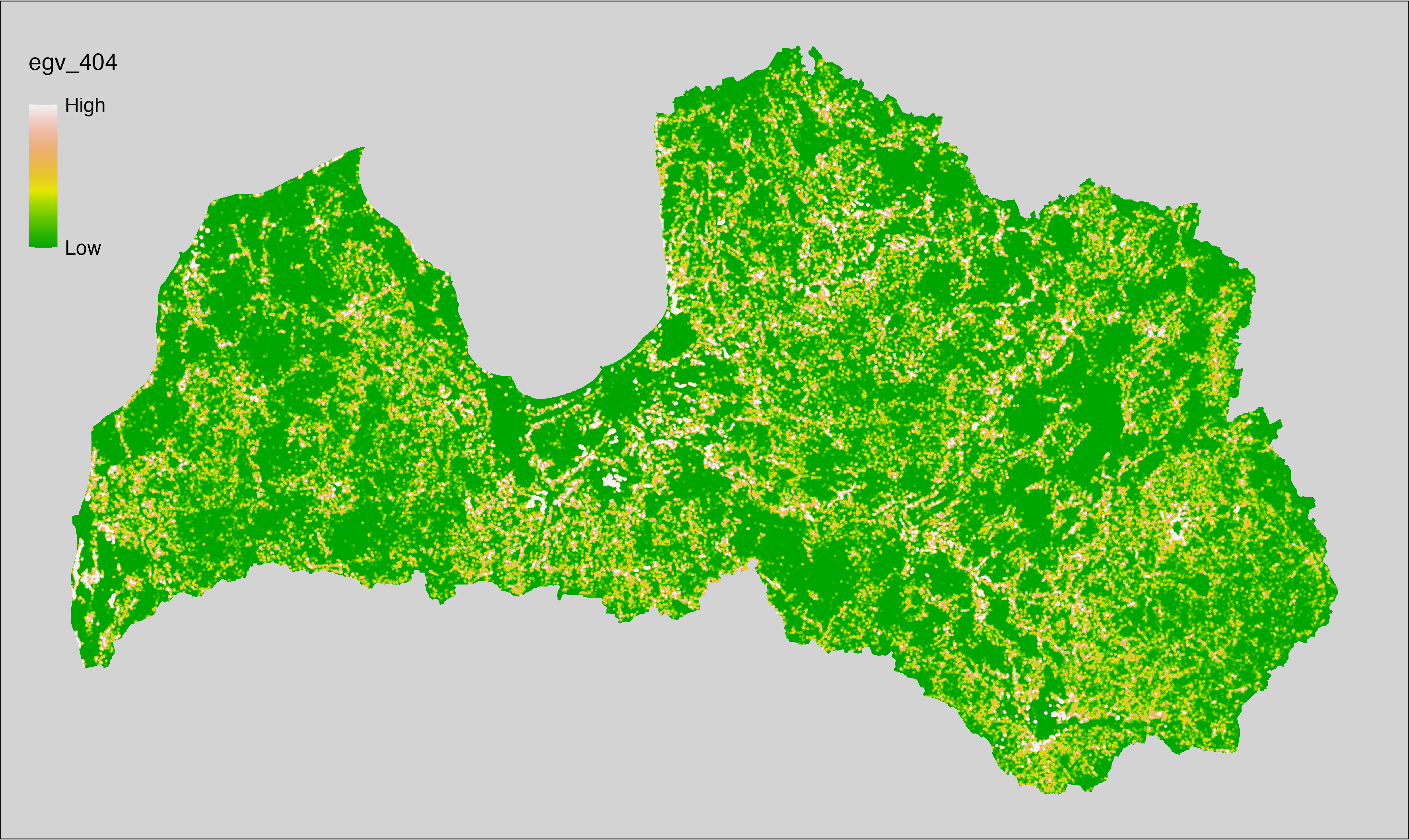
6.405 General_AllotmentGardens_r1250
filename: General_AllotmentGardens_r1250.tif
layername: egv_405
English name: Fractional cover of Allotment gardens within the 1.25 km landscape
Latvian name: Vasarnīcu kompleksu platības īpatsvars 1,25 km ainavā
Procedure: The cover fraction within a radius of 1250 m around the analysis grid cell
is calculated as the area-weighted sum of the analysis cells inside
the buffer, using the workflow egvtools::radius_function(). During the calculation of the landscape
metric, inverse distance weighted (power = 2) gap filling on the output is
applied to ensure no missing values at the edges. Then the layer is
rewritten to set its name. Finally, the layer is standardised by
subtracting the arithmetic mean and dividing by the root mean squared error.
Code
# libs ----
if(!require(terra)) {install.packages("terra"); require(terra)}
if(!require(egvtools)) {remotes::install_github("aavotins/egvtools"); require(egvtools)}
# Templates -----
template100=rast("./Templates/TemplateRasters/LV100m_10km.tif")
# radii ----
radius_function(
kvadrati_path = "./Templates/TemplateGrids/tiles/",
radii_path = "./Templates/TemplateGridPoints/tiles/",
tikls100_path = "./Templates/TemplateGrids/tikls100_sauzeme.parquet",
template_path = "./Templates/TemplateRasters/LV100m_10km.tif",
input_layers = c("./RasterGrids_100m/2024/RAW/General_AllotmentGardens_cell.tif"),
layer_prefixes = c("General_AllotmentGardens"),
output_dir = "./RasterGrids_100m/2024/RAW/",
n_workers = 6,
radii = c("r1250"),
radius_mode = "sparse",
extract_fun = "mean",
fill_missing = TRUE,
IDW_weight = 2,
future_max_size = 40 * 1024^3)
# General_AllotmentGardens_r1250.tif egv_405
slanis=rast("./RasterGrids_100m/2024/RAW/General_AllotmentGardens_r1250.tif")
names(slanis)="egv_405"
slanis2=project(slanis,template100)
writeRaster(slanis2,
"./RasterGrids_100m/2024/RAW/General_AllotmentGardens_r1250.tif",
overwrite=TRUE)
# standardisation ----
if(!require(terra)) {install.packages("terra"); require(terra)}
if(!require(tidyverse)) {install.packages("tidyverse"); require(tidyverse)}
nosaukums="General_AllotmentGardens_r1250.tif"
ielasisanas_cels=paste0("./RasterGrids_100m/2024/RAW/",nosaukums)
saglabasanas_cels=paste0("./RasterGrids_100m/2024/Scaled/",nosaukums)
slanis=rast(ielasisanas_cels)
videjais=global(slanis,fun="mean",na.rm=TRUE)
centrets=slanis-videjais[,1]
standartnovirze=terra::global(centrets,fun="rms",na.rm=TRUE)
merogots=centrets/standartnovirze[,1]
writeRaster(merogots,
filename=saglabasanas_cels,
overwrite=TRUE)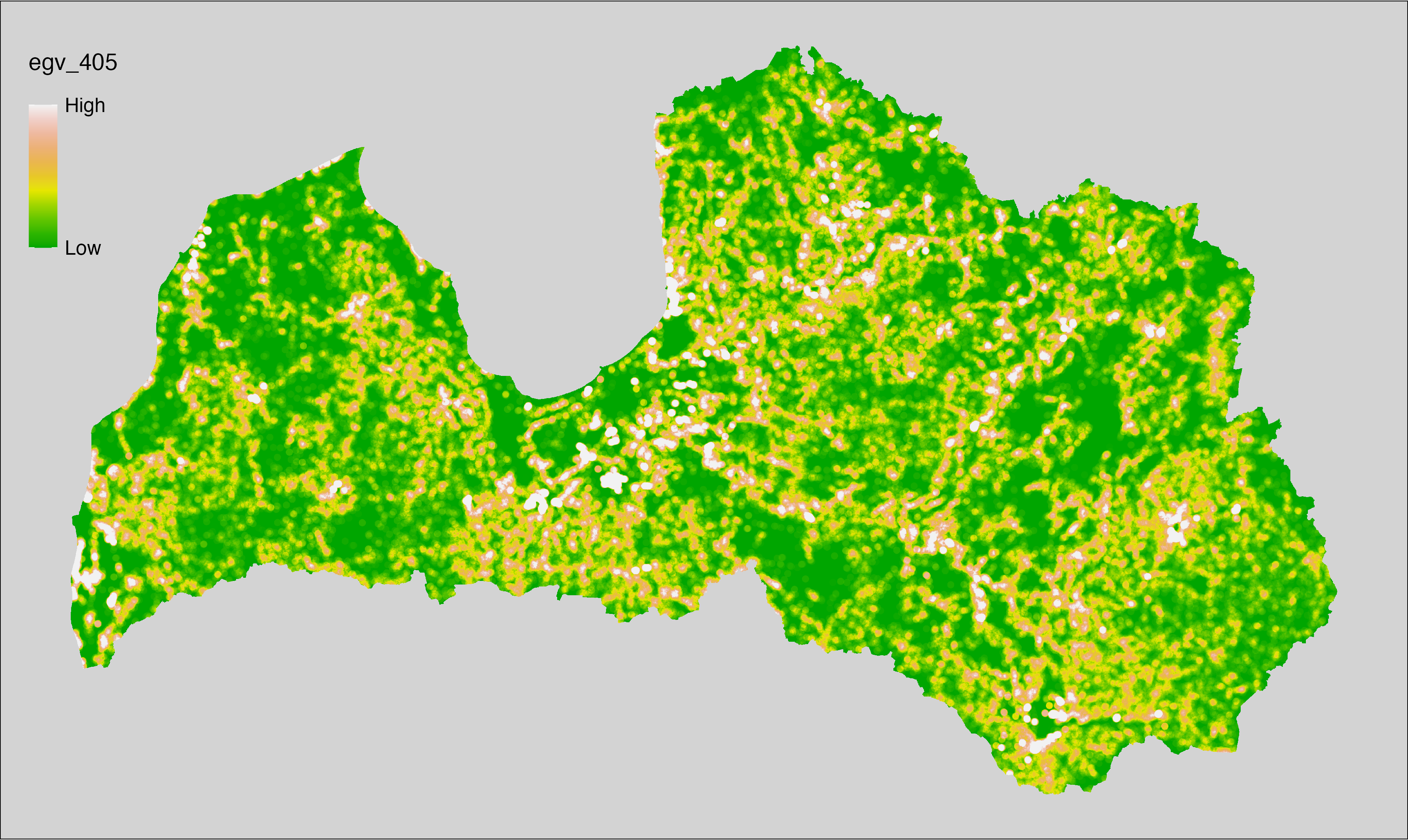
6.406 General_AllotmentGardens_r3000
filename: General_AllotmentGardens_r3000.tif
layername: egv_406
English name: Fractional cover of Allotment gardens within the 3 km landscape
Latvian name: Vasarnīcu kompleksu platības īpatsvars 3 km ainavā
Procedure: The cover fraction within a radius of 3000 m around the analysis grid cell
is calculated as the area-weighted sum of the analysis cells inside
the buffer, using the workflow egvtools::radius_function(). During the calculation of the landscape
metric, inverse distance weighted (power = 2) gap filling on the output is
applied to ensure no missing values at the edges. Then the layer is
rewritten to set its name. Finally, the layer is standardised by
subtracting the arithmetic mean and dividing by the root mean squared error.
Code
# libs ----
if(!require(terra)) {install.packages("terra"); require(terra)}
if(!require(egvtools)) {remotes::install_github("aavotins/egvtools"); require(egvtools)}
# Templates -----
template100=rast("./Templates/TemplateRasters/LV100m_10km.tif")
# radii ----
radius_function(
kvadrati_path = "./Templates/TemplateGrids/tiles/",
radii_path = "./Templates/TemplateGridPoints/tiles/",
tikls100_path = "./Templates/TemplateGrids/tikls100_sauzeme.parquet",
template_path = "./Templates/TemplateRasters/LV100m_10km.tif",
input_layers = c("./RasterGrids_100m/2024/RAW/General_AllotmentGardens_cell.tif"),
layer_prefixes = c("General_AllotmentGardens"),
output_dir = "./RasterGrids_100m/2024/RAW/",
n_workers = 6,
radii = c("r3000"),
radius_mode = "sparse",
extract_fun = "mean",
fill_missing = TRUE,
IDW_weight = 2,
future_max_size = 40 * 1024^3)
# General_AllotmentGardens_r3000.tif egv_406
slanis=rast("./RasterGrids_100m/2024/RAW/General_AllotmentGardens_r3000.tif")
names(slanis)="egv_406"
slanis2=project(slanis,template100)
writeRaster(slanis2,
"./RasterGrids_100m/2024/RAW/General_AllotmentGardens_r3000.tif",
overwrite=TRUE)
# standardisation ----
if(!require(terra)) {install.packages("terra"); require(terra)}
if(!require(tidyverse)) {install.packages("tidyverse"); require(tidyverse)}
nosaukums="General_AllotmentGardens_r3000.tif"
ielasisanas_cels=paste0("./RasterGrids_100m/2024/RAW/",nosaukums)
saglabasanas_cels=paste0("./RasterGrids_100m/2024/Scaled/",nosaukums)
slanis=rast(ielasisanas_cels)
videjais=global(slanis,fun="mean",na.rm=TRUE)
centrets=slanis-videjais[,1]
standartnovirze=terra::global(centrets,fun="rms",na.rm=TRUE)
merogots=centrets/standartnovirze[,1]
writeRaster(merogots,
filename=saglabasanas_cels,
overwrite=TRUE)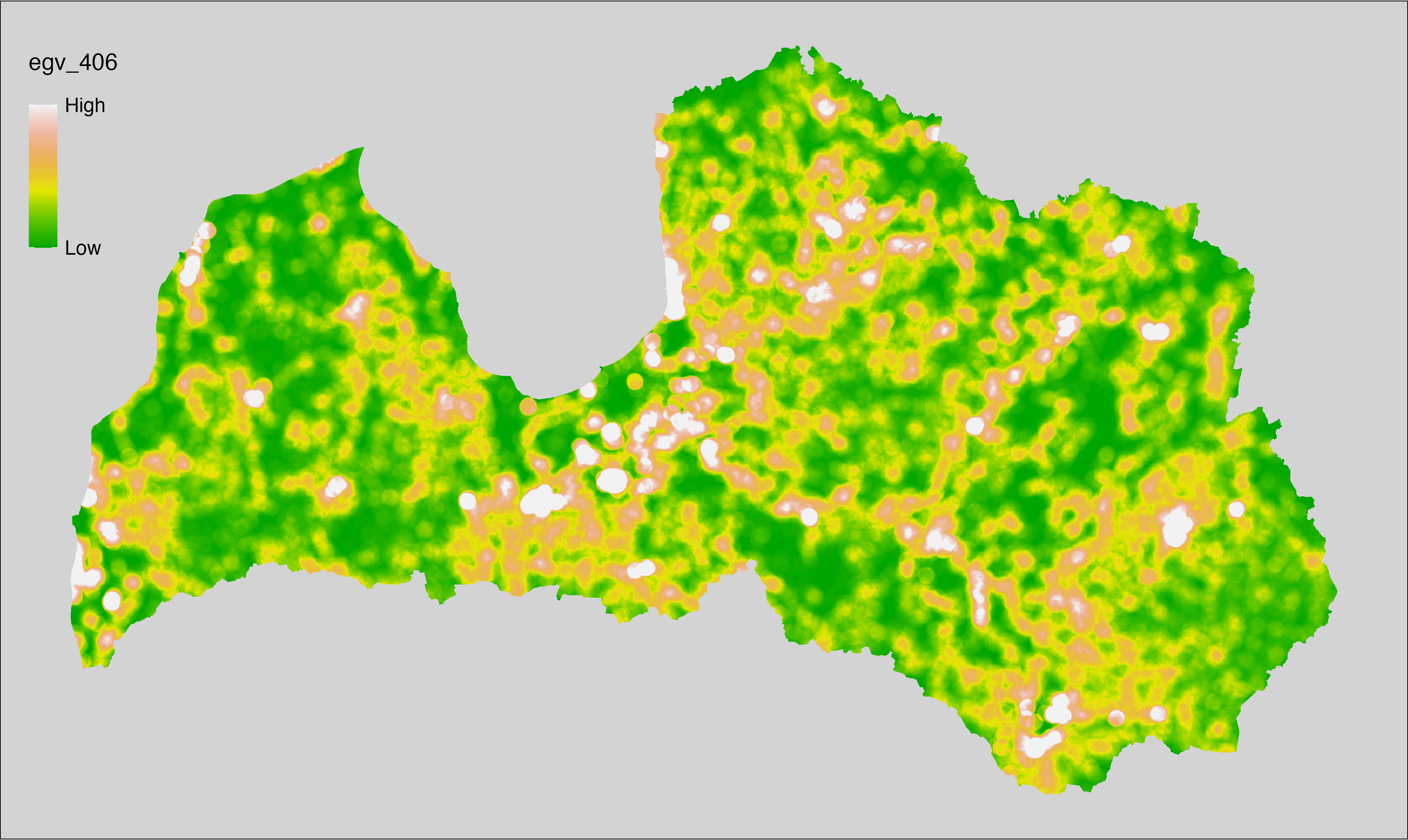
6.407 General_AllotmentGardens_r10000
filename: General_AllotmentGardens_r10000.tif
layername: egv_407
English name: Fractional cover of Allotment gardens within the 10 km landscape
Latvian name: Vasarnīcu kompleksu platības īpatsvars 10 km ainavā
Procedure: The cover fraction within a radius of 10000 m around the analysis grid cell
is calculated as the area-weighted sum of the analysis cells inside
the buffer, using the workflow egvtools::radius_function(). During the calculation of the landscape
metric, inverse distance weighted (power = 2) gap filling on the output is
applied to ensure no missing values at the edges. Then the layer is
rewritten to set its name. Finally, the layer is standardised by
subtracting the arithmetic mean and dividing by the root mean squared error.
Code
# libs ----
if(!require(terra)) {install.packages("terra"); require(terra)}
if(!require(egvtools)) {remotes::install_github("aavotins/egvtools"); require(egvtools)}
# Templates -----
template100=rast("./Templates/TemplateRasters/LV100m_10km.tif")
# radii ----
radius_function(
kvadrati_path = "./Templates/TemplateGrids/tiles/",
radii_path = "./Templates/TemplateGridPoints/tiles/",
tikls100_path = "./Templates/TemplateGrids/tikls100_sauzeme.parquet",
template_path = "./Templates/TemplateRasters/LV100m_10km.tif",
input_layers = c("./RasterGrids_100m/2024/RAW/General_AllotmentGardens_cell.tif"),
layer_prefixes = c("General_AllotmentGardens"),
output_dir = "./RasterGrids_100m/2024/RAW/",
n_workers = 6,
radii = c("r10000"),
radius_mode = "sparse",
extract_fun = "mean",
fill_missing = TRUE,
IDW_weight = 2,
future_max_size = 40 * 1024^3)
# General_AllotmentGardens_r10000.tif egv_407
slanis=rast("./RasterGrids_100m/2024/RAW/General_AllotmentGardens_r10000.tif")
names(slanis)="egv_407"
slanis2=project(slanis,template100)
writeRaster(slanis2,
"./RasterGrids_100m/2024/RAW/General_AllotmentGardens_r10000.tif",
overwrite=TRUE)
# standardisation ----
if(!require(terra)) {install.packages("terra"); require(terra)}
if(!require(tidyverse)) {install.packages("tidyverse"); require(tidyverse)}
nosaukums="General_AllotmentGardens_r10000.tif"
ielasisanas_cels=paste0("./RasterGrids_100m/2024/RAW/",nosaukums)
saglabasanas_cels=paste0("./RasterGrids_100m/2024/Scaled/",nosaukums)
slanis=rast(ielasisanas_cels)
videjais=global(slanis,fun="mean",na.rm=TRUE)
centrets=slanis-videjais[,1]
standartnovirze=terra::global(centrets,fun="rms",na.rm=TRUE)
merogots=centrets/standartnovirze[,1]
writeRaster(merogots,
filename=saglabasanas_cels,
overwrite=TRUE)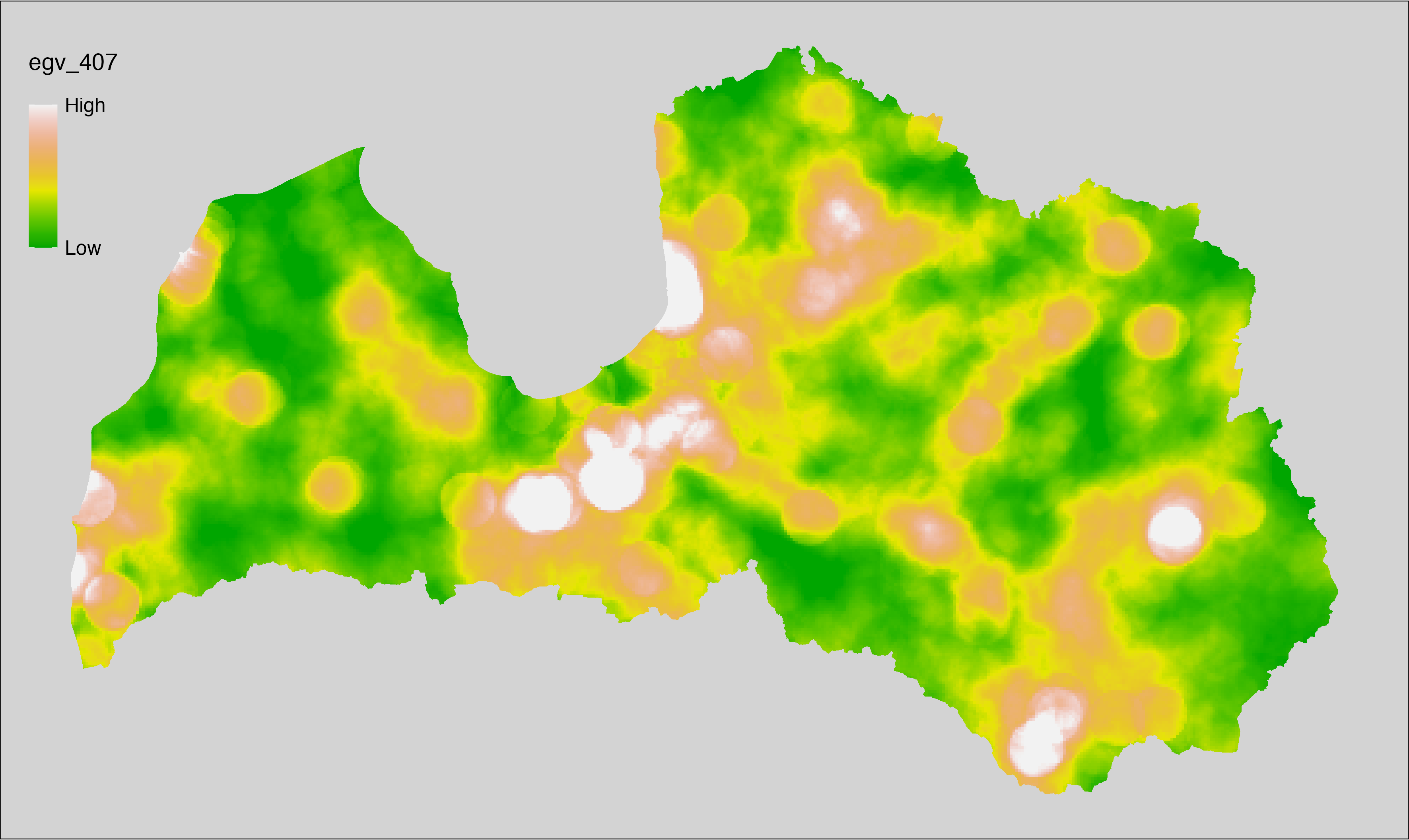
6.408 General_BareSoilQuarry_cell
filename: General_BareSoilQuarry_cell.tif
layername: egv_408
English name: Fractional cover of areas with Bare Soil, Quarries within the analysis cell (1 ha)
Latvian name: Atklātas augsnes un karjeru platības īpatsvars analīzes šūnā (1 ha)
Procedure: First, the bare soil and quarry areas from the Landscape
classification are selected (value 800 is reclassified to value 1;
all others are set to 0). The resulting layer
is then aggregated to EGV resolution using the workflow egvtools::input2egv(), which
calculates the arithmetic mean to determine the cover fraction. During
aggregation, inverse distance weighted (power = 2) gap filling on the output is
applied to ensure no missing values at the edges. Finally, the layer is
standardised by subtracting the arithmetic mean and dividing by the root mean squared
error.
Code
# libs ----
if(!require(egvtools)) {remotes::install_github("aavotins/egvtools"); require(egvtools)}
if(!require(terra)) {install.packages("terra"); require(terra)}
if(!require(sf)) {install.packages("sf"); require(sf)}
if(!require(tidyverse)) {install.packages("tidyverse"); require(tidyverse)}
if(!require(sfarrow)) {install.packages("sfarrow"); require(sfarrow)}
if(!require(readxl)) {install.packages("readxl"); require(readxl)}
if(!require(raster)) {install.packages("raster"); require(raster)}
if(!require(fasterize)) {install.packages("fasterize"); require(fasterize)}
# templates ----
template100=rast("./Templates/TemplateRasters/LV100m_10km.tif")
template10=rast("./Templates/TemplateRasters/LV10m_10km.tif")
rastrs10=raster(template10)
nulls10=rast("./Templates/TemplateRasters/nulls_LV10m_10km.tif")
nulls100=rast("./Templates/TemplateRasters/nulls_LV100m_10km.tif")
# simple landscape ----
simple_landscape=rast("RasterGrids_10m/2024/Ainava_vienk_mask.tif")
# General_BareSoilQuarry_cell.tif egv_408 ----
baresoilquerry=ifel(simple_landscape==800,1,0)
i2e_rez=egvtools::input2egv(input=baresoilquerry,
egv_template= "./Templates/TemplateRasters/LV100m_10km.tif",
summary_function = "average",
missing_job = "FillOutput",
outlocation = "./RasterGrids_100m/2024/RAW/",
outfilename = "General_BareSoilQuarry_cell.tif",
layername = "egv_408",
idw_weight = 2,
plot_gaps = FALSE,plot_final = TRUE)
i2e_rez
rm(baresoilquerry)
rm(i2e_rez)
# standardisation ----
if(!require(terra)) {install.packages("terra"); require(terra)}
if(!require(tidyverse)) {install.packages("tidyverse"); require(tidyverse)}
nosaukums="General_BareSoilQuarry_cell.tif"
ielasisanas_cels=paste0("./RasterGrids_100m/2024/RAW/",nosaukums)
saglabasanas_cels=paste0("./RasterGrids_100m/2024/Scaled/",nosaukums)
slanis=rast(ielasisanas_cels)
videjais=global(slanis,fun="mean",na.rm=TRUE)
centrets=slanis-videjais[,1]
standartnovirze=terra::global(centrets,fun="rms",na.rm=TRUE)
merogots=centrets/standartnovirze[,1]
writeRaster(merogots,
filename=saglabasanas_cels,
overwrite=TRUE)
6.409 General_BareSoilQuarry_r500
filename: General_BareSoilQuarry_r500.tif
layername: egv_409
English name: Fractional cover of areas with Bare Soil, Quarries within the 0.5 km landscape
Latvian name: Atklātas augsnes un karjeru platības īpatsvars 0,5 km ainavā
Procedure: The cover fraction within a radius of 500 m around the analysis grid cell is
calculated as the area-weighted sum of the analysis cells inside the
buffer, using the workflow egvtools::radius_function(). During the calculation of the landscape metric,
inverse distance weighted (power = 2) gap filling on the output is applied
to ensure no missing values at the edges. Then the layer is rewritten to set
its name. Finally, the layer is standardised by subtracting the arithmetic
mean and dividing by the root mean squared error.
Code
# libs ----
if(!require(terra)) {install.packages("terra"); require(terra)}
if(!require(egvtools)) {remotes::install_github("aavotins/egvtools"); require(egvtools)}
# Templates -----
template100=rast("./Templates/TemplateRasters/LV100m_10km.tif")
# radii ----
radius_function(
kvadrati_path = "./Templates/TemplateGrids/tiles/",
radii_path = "./Templates/TemplateGridPoints/tiles/",
tikls100_path = "./Templates/TemplateGrids/tikls100_sauzeme.parquet",
template_path = "./Templates/TemplateRasters/LV100m_10km.tif",
input_layers = c("./RasterGrids_100m/2024/RAW/General_BareSoilQuarry_cell.tif"),
layer_prefixes = c("General_BareSoilQuarry"),
output_dir = "./RasterGrids_100m/2024/RAW/",
n_workers = 6,
radii = c("r500"),
radius_mode = "sparse",
extract_fun = "mean",
fill_missing = TRUE,
IDW_weight = 2,
future_max_size = 40 * 1024^3)
# General_BareSoilQuarry_r500.tif egv_409
slanis=rast("./RasterGrids_100m/2024/RAW/General_BareSoilQuarry_r500.tif")
names(slanis)="egv_409"
slanis2=project(slanis,template100)
writeRaster(slanis2,
"./RasterGrids_100m/2024/RAW/General_BareSoilQuarry_r500.tif",
overwrite=TRUE)
# standardisation ----
if(!require(terra)) {install.packages("terra"); require(terra)}
if(!require(tidyverse)) {install.packages("tidyverse"); require(tidyverse)}
nosaukums="General_BareSoilQuarry_r500.tif"
ielasisanas_cels=paste0("./RasterGrids_100m/2024/RAW/",nosaukums)
saglabasanas_cels=paste0("./RasterGrids_100m/2024/Scaled/",nosaukums)
slanis=rast(ielasisanas_cels)
videjais=global(slanis,fun="mean",na.rm=TRUE)
centrets=slanis-videjais[,1]
standartnovirze=terra::global(centrets,fun="rms",na.rm=TRUE)
merogots=centrets/standartnovirze[,1]
writeRaster(merogots,
filename=saglabasanas_cels,
overwrite=TRUE)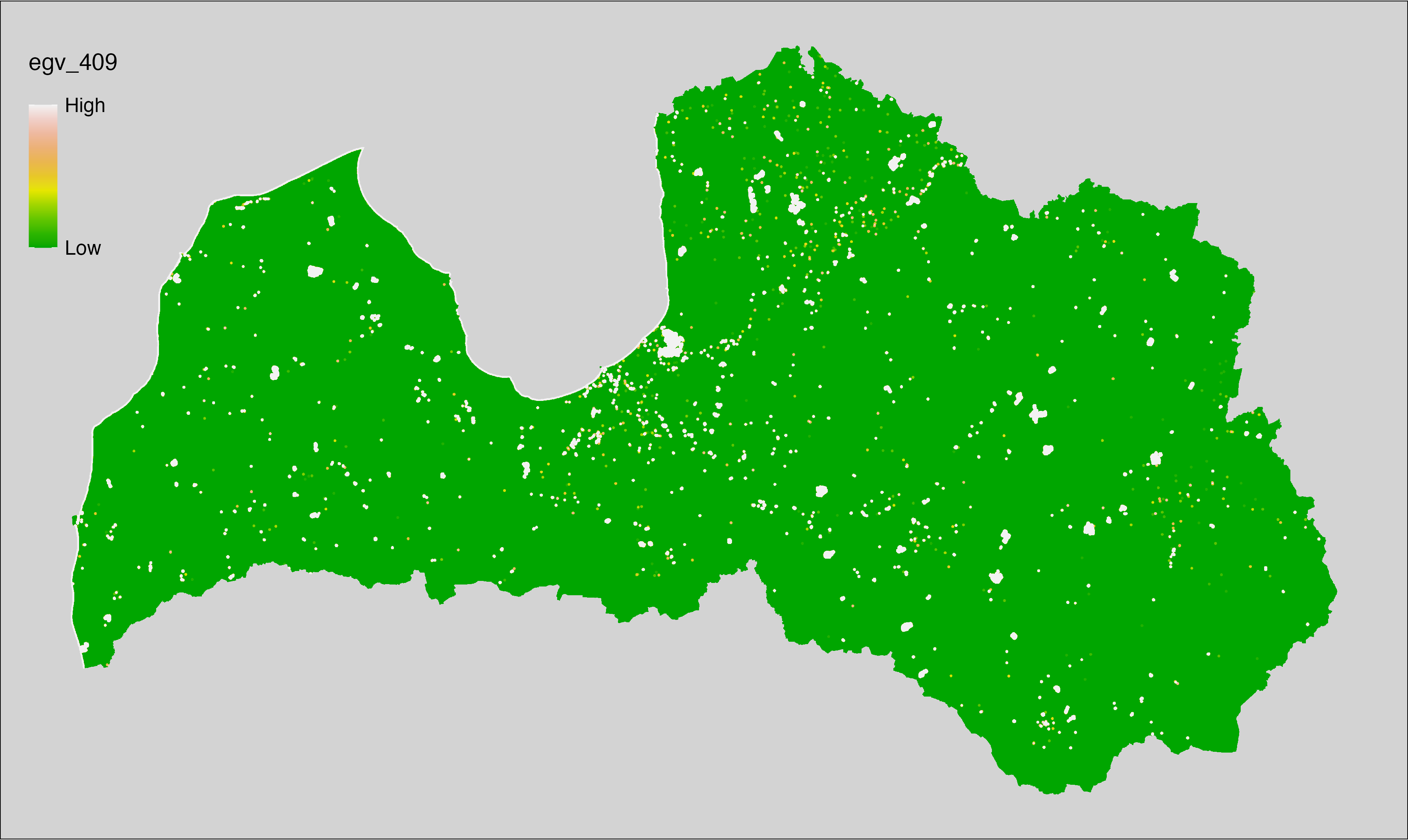
6.410 General_BareSoilQuarry_r1250
filename: General_BareSoilQuarry_r1250.tif
layername: egv_410
English name: Fractional cover of areas with Bare Soil, Quarries within the 1.25 km landscape
Latvian name: Atklātas augsnes un karjeru platības īpatsvars 1,25 km ainavā
Procedure: The cover fraction within a radius of 1250 m around the analysis grid cell
is calculated as the area-weighted sum of the analysis cells inside
the buffer, using the workflow egvtools::radius_function(). During the calculation of the landscape
metric, inverse distance weighted (power = 2) gap filling on the output is
applied to ensure no missing values at the edges. Then the layer is
rewritten to set its name. Finally, the layer is standardised by
subtracting the arithmetic mean and dividing by the root mean squared error.
Code
# libs ----
if(!require(terra)) {install.packages("terra"); require(terra)}
if(!require(egvtools)) {remotes::install_github("aavotins/egvtools"); require(egvtools)}
# Templates -----
template100=rast("./Templates/TemplateRasters/LV100m_10km.tif")
# radii ----
radius_function(
kvadrati_path = "./Templates/TemplateGrids/tiles/",
radii_path = "./Templates/TemplateGridPoints/tiles/",
tikls100_path = "./Templates/TemplateGrids/tikls100_sauzeme.parquet",
template_path = "./Templates/TemplateRasters/LV100m_10km.tif",
input_layers = c("./RasterGrids_100m/2024/RAW/General_BareSoilQuarry_cell.tif"),
layer_prefixes = c("General_BareSoilQuarry"),
output_dir = "./RasterGrids_100m/2024/RAW/",
n_workers = 6,
radii = c("r1250"),
radius_mode = "sparse",
extract_fun = "mean",
fill_missing = TRUE,
IDW_weight = 2,
future_max_size = 40 * 1024^3)
# General_BareSoilQuarry_r1250.tif egv_410
slanis=rast("./RasterGrids_100m/2024/RAW/General_BareSoilQuarry_r1250.tif")
names(slanis)="egv_410"
slanis2=project(slanis,template100)
writeRaster(slanis2,
"./RasterGrids_100m/2024/RAW/General_BareSoilQuarry_r1250.tif",
overwrite=TRUE)
# standardisation ----
if(!require(terra)) {install.packages("terra"); require(terra)}
if(!require(tidyverse)) {install.packages("tidyverse"); require(tidyverse)}
nosaukums="General_BareSoilQuarry_r1250.tif"
ielasisanas_cels=paste0("./RasterGrids_100m/2024/RAW/",nosaukums)
saglabasanas_cels=paste0("./RasterGrids_100m/2024/Scaled/",nosaukums)
slanis=rast(ielasisanas_cels)
videjais=global(slanis,fun="mean",na.rm=TRUE)
centrets=slanis-videjais[,1]
standartnovirze=terra::global(centrets,fun="rms",na.rm=TRUE)
merogots=centrets/standartnovirze[,1]
writeRaster(merogots,
filename=saglabasanas_cels,
overwrite=TRUE)
6.411 General_BareSoilQuarry_r3000
filename: General_BareSoilQuarry_r3000.tif
layername: egv_411
English name: Fractional cover of areas with Bare Soil, Quarries within the 3 km landscape
Latvian name: Atklātas augsnes un karjeru platības īpatsvars 3 km ainavā
Procedure: The cover fraction within a radius of 3000 m around the analysis grid cell
is calculated as the area-weighted sum of the analysis cells inside
the buffer, using the workflow egvtools::radius_function(). During the calculation of the landscape
metric, inverse distance weighted (power = 2) gap filling on the output is
applied to ensure no missing values at the edges. Then the layer is
rewritten to set its name. Finally, the layer is standardised by
subtracting the arithmetic mean and dividing by the root mean squared error.
Code
# libs ----
if(!require(terra)) {install.packages("terra"); require(terra)}
if(!require(egvtools)) {remotes::install_github("aavotins/egvtools"); require(egvtools)}
# Templates -----
template100=rast("./Templates/TemplateRasters/LV100m_10km.tif")
# radii ----
radius_function(
kvadrati_path = "./Templates/TemplateGrids/tiles/",
radii_path = "./Templates/TemplateGridPoints/tiles/",
tikls100_path = "./Templates/TemplateGrids/tikls100_sauzeme.parquet",
template_path = "./Templates/TemplateRasters/LV100m_10km.tif",
input_layers = c("./RasterGrids_100m/2024/RAW/General_BareSoilQuarry_cell.tif"),
layer_prefixes = c("General_BareSoilQuarry"),
output_dir = "./RasterGrids_100m/2024/RAW/",
n_workers = 6,
radii = c("r3000"),
radius_mode = "sparse",
extract_fun = "mean",
fill_missing = TRUE,
IDW_weight = 2,
future_max_size = 40 * 1024^3)
# General_BareSoilQuarry_r3000.tif egv_411
slanis=rast("./RasterGrids_100m/2024/RAW/General_BareSoilQuarry_r3000.tif")
names(slanis)="egv_411"
slanis2=project(slanis,template100)
writeRaster(slanis2,
"./RasterGrids_100m/2024/RAW/General_BareSoilQuarry_r3000.tif",
overwrite=TRUE)
# standardisation ----
if(!require(terra)) {install.packages("terra"); require(terra)}
if(!require(tidyverse)) {install.packages("tidyverse"); require(tidyverse)}
nosaukums="General_BareSoilQuarry_r3000.tif"
ielasisanas_cels=paste0("./RasterGrids_100m/2024/RAW/",nosaukums)
saglabasanas_cels=paste0("./RasterGrids_100m/2024/Scaled/",nosaukums)
slanis=rast(ielasisanas_cels)
videjais=global(slanis,fun="mean",na.rm=TRUE)
centrets=slanis-videjais[,1]
standartnovirze=terra::global(centrets,fun="rms",na.rm=TRUE)
merogots=centrets/standartnovirze[,1]
writeRaster(merogots,
filename=saglabasanas_cels,
overwrite=TRUE)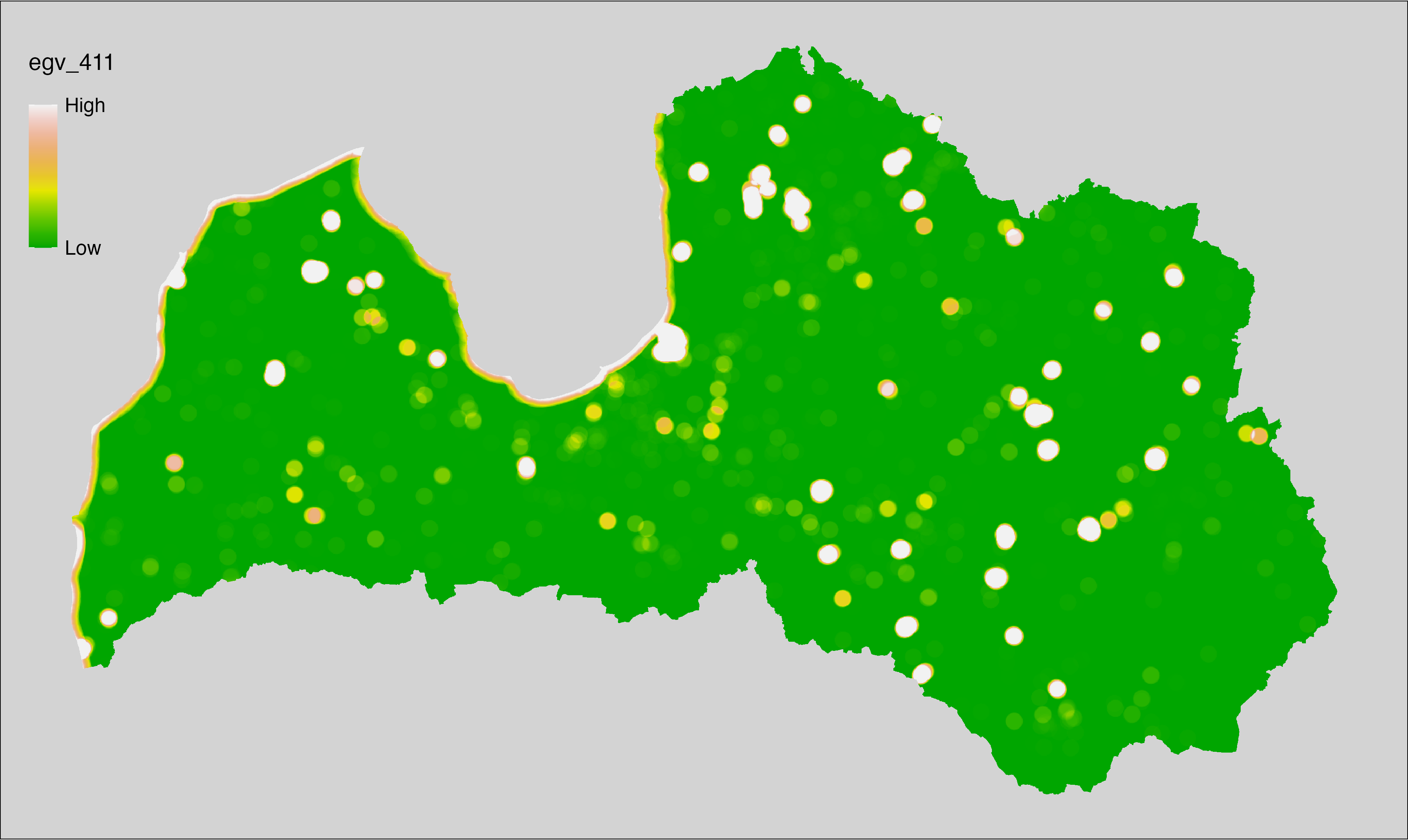
6.412 General_BareSoilQuarry_r10000
filename: General_BareSoilQuarry_r10000.tif
layername: egv_412
English name: Fractional cover of areas with Bare Soil, Quarries within the 10 km landscape
Latvian name: Atklātas augsnes un karjeru platības īpatsvars 10 km ainavā
Procedure: The cover fraction within a radius of 10000 m around the analysis grid cell
is calculated as the area-weighted sum of the analysis cells inside
the buffer, using the workflow egvtools::radius_function(). During the calculation of the landscape
metric, inverse distance weighted (power = 2) gap filling on the output is
applied to ensure no missing values at the edges. Then the layer is
rewritten to set its name. Finally, the layer is standardised by
subtracting the arithmetic mean and dividing by the root mean squared error.
Code
# libs ----
if(!require(terra)) {install.packages("terra"); require(terra)}
if(!require(egvtools)) {remotes::install_github("aavotins/egvtools"); require(egvtools)}
# Templates -----
template100=rast("./Templates/TemplateRasters/LV100m_10km.tif")
# radii ----
radius_function(
kvadrati_path = "./Templates/TemplateGrids/tiles/",
radii_path = "./Templates/TemplateGridPoints/tiles/",
tikls100_path = "./Templates/TemplateGrids/tikls100_sauzeme.parquet",
template_path = "./Templates/TemplateRasters/LV100m_10km.tif",
input_layers = c("./RasterGrids_100m/2024/RAW/General_BareSoilQuarry_cell.tif"),
layer_prefixes = c("General_BareSoilQuarry"),
output_dir = "./RasterGrids_100m/2024/RAW/",
n_workers = 6,
radii = c("r10000"),
radius_mode = "sparse",
extract_fun = "mean",
fill_missing = TRUE,
IDW_weight = 2,
future_max_size = 40 * 1024^3)
# General_BareSoilQuarry_r10000.tif egv_412
slanis=rast("./RasterGrids_100m/2024/RAW/General_BareSoilQuarry_r10000.tif")
names(slanis)="egv_412"
slanis2=project(slanis,template100)
writeRaster(slanis2,
"./RasterGrids_100m/2024/RAW/General_BareSoilQuarry_r10000.tif",
overwrite=TRUE)
# standardisation ----
if(!require(terra)) {install.packages("terra"); require(terra)}
if(!require(tidyverse)) {install.packages("tidyverse"); require(tidyverse)}
nosaukums="General_BareSoilQuarry_r10000.tif"
ielasisanas_cels=paste0("./RasterGrids_100m/2024/RAW/",nosaukums)
saglabasanas_cels=paste0("./RasterGrids_100m/2024/Scaled/",nosaukums)
slanis=rast(ielasisanas_cels)
videjais=global(slanis,fun="mean",na.rm=TRUE)
centrets=slanis-videjais[,1]
standartnovirze=terra::global(centrets,fun="rms",na.rm=TRUE)
merogots=centrets/standartnovirze[,1]
writeRaster(merogots,
filename=saglabasanas_cels,
overwrite=TRUE)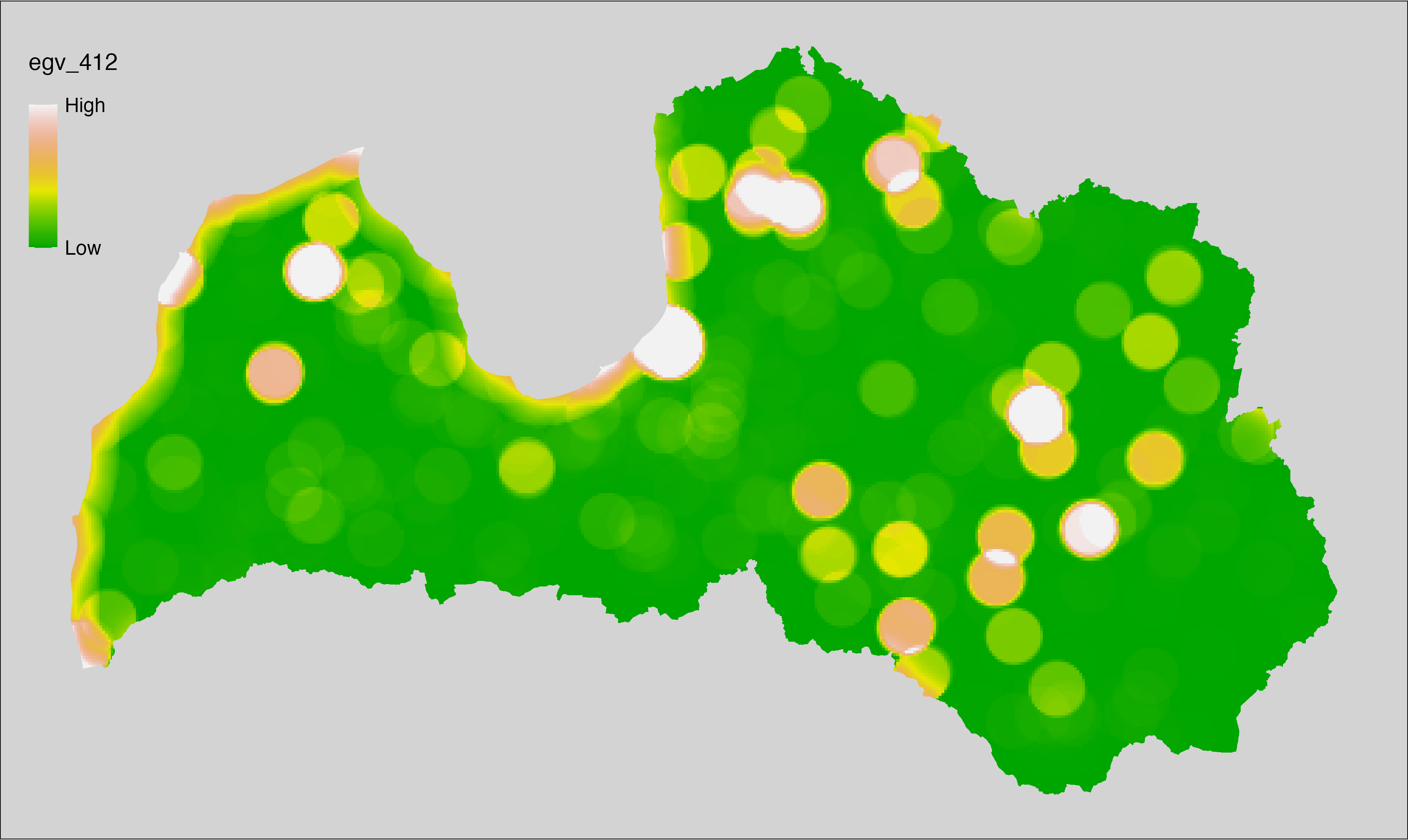
6.413 General_Builtup_cell
filename: General_Builtup_cell.tif
layername: egv_413
English name: Fractional cover of Built-Up areas within the analysis cell (1 ha)
Latvian name: Apbūves platības īpatsvars analīzes šūnā (1 ha)
Procedure: First, the built-up areas from the Landscape classification
are selected (value 500 is reclassified to value 1; all others are set to 0). The resulting layer
is then aggregated to EGV resolution using the workflow egvtools::input2egv(), which
calculates the arithmetic mean to determine the cover fraction. During
aggregation, inverse distance weighted (power = 2) gap filling on the output is
applied to ensure no missing values at the edges. Finally, the layer is
standardised by subtracting the arithmetic mean and dividing by the root mean squared
error.
Code
# libs ----
if(!require(egvtools)) {remotes::install_github("aavotins/egvtools"); require(egvtools)}
if(!require(terra)) {install.packages("terra"); require(terra)}
if(!require(sf)) {install.packages("sf"); require(sf)}
if(!require(tidyverse)) {install.packages("tidyverse"); require(tidyverse)}
if(!require(sfarrow)) {install.packages("sfarrow"); require(sfarrow)}
if(!require(readxl)) {install.packages("readxl"); require(readxl)}
if(!require(raster)) {install.packages("raster"); require(raster)}
if(!require(fasterize)) {install.packages("fasterize"); require(fasterize)}
# templates ----
template100=rast("./Templates/TemplateRasters/LV100m_10km.tif")
template10=rast("./Templates/TemplateRasters/LV10m_10km.tif")
rastrs10=raster(template10)
nulls10=rast("./Templates/TemplateRasters/nulls_LV10m_10km.tif")
nulls100=rast("./Templates/TemplateRasters/nulls_LV100m_10km.tif")
# simple landscape ----
simple_landscape=rast("RasterGrids_10m/2024/Ainava_vienk_mask.tif")
# General_Builtup_cell.tif egv_413 ----
builtup=ifel(simple_landscape==500,1,0)
i2e_rez=egvtools::input2egv(input=builtup,
egv_template= "./Templates/TemplateRasters/LV100m_10km.tif",
summary_function = "average",
missing_job = "FillOutput",
outlocation = "./RasterGrids_100m/2024/RAW/",
outfilename = "General_Builtup_cell.tif",
layername = "egv_413",
idw_weight = 2,
plot_gaps = FALSE,plot_final = TRUE)
i2e_rez
rm(builtup)
rm(i2e_rez)
# standardisation ----
if(!require(terra)) {install.packages("terra"); require(terra)}
if(!require(tidyverse)) {install.packages("tidyverse"); require(tidyverse)}
nosaukums="General_Builtup_cell.tif"
ielasisanas_cels=paste0("./RasterGrids_100m/2024/RAW/",nosaukums)
saglabasanas_cels=paste0("./RasterGrids_100m/2024/Scaled/",nosaukums)
slanis=rast(ielasisanas_cels)
videjais=global(slanis,fun="mean",na.rm=TRUE)
centrets=slanis-videjais[,1]
standartnovirze=terra::global(centrets,fun="rms",na.rm=TRUE)
merogots=centrets/standartnovirze[,1]
writeRaster(merogots,
filename=saglabasanas_cels,
overwrite=TRUE)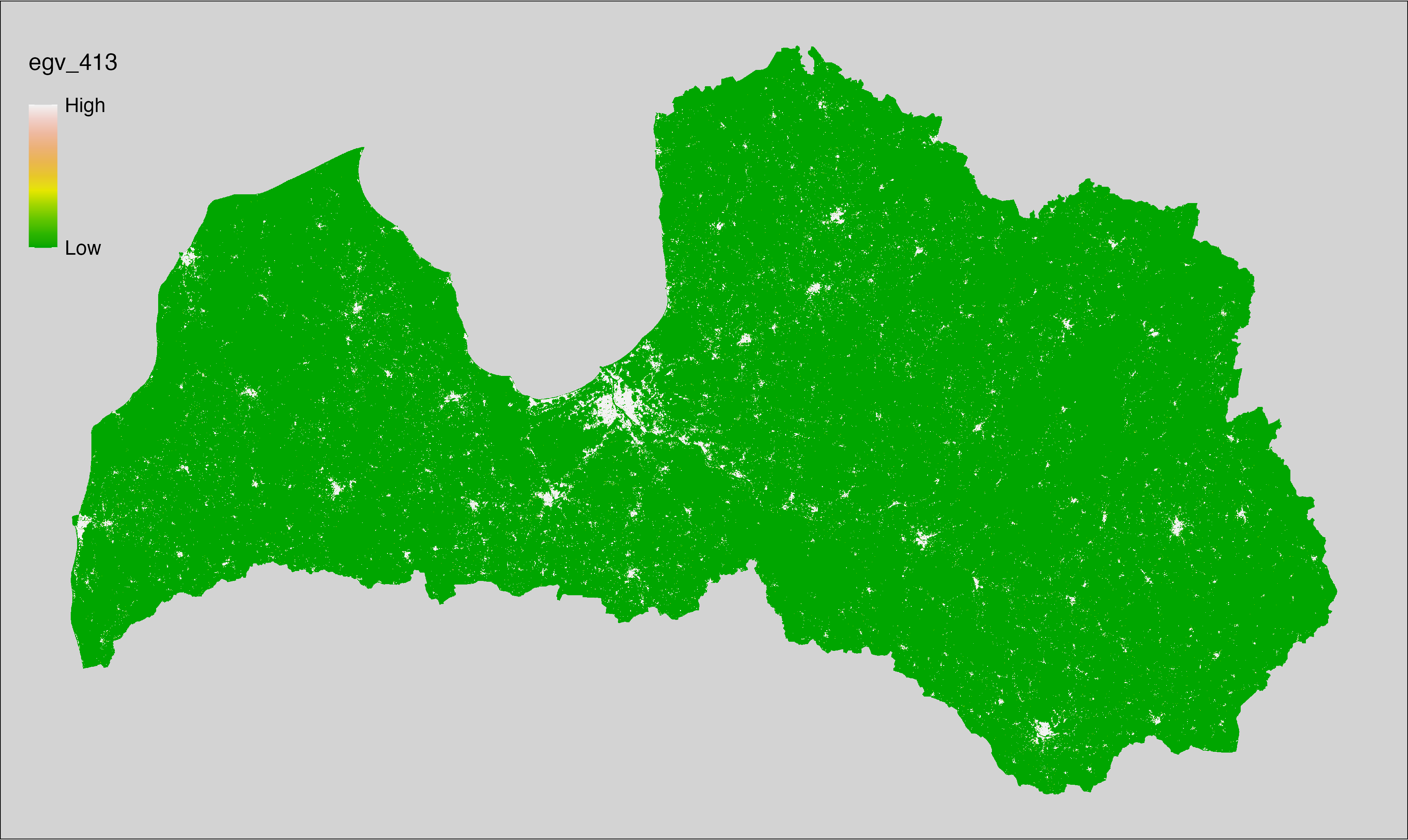
6.414 General_Builtup_r500
filename: General_Builtup_r500.tif
layername: egv_414
English name: Fractional cover of Built-Up areas within the 0.5 km landscape
Latvian name: Apbūves platības īpatsvars 0,5 km ainavā
Procedure: The cover fraction within a radius of 500 m around the analysis grid cell is
calculated as the area-weighted sum of the analysis cells inside the
buffer, using the workflow egvtools::radius_function(). During the calculation of the landscape metric,
inverse distance weighted (power = 2) gap filling on the output is applied
to ensure no missing values at the edges. Then the layer is rewritten to set
its name. Finally, the layer is standardised by subtracting the arithmetic
mean and dividing by the root mean squared error.
Code
# libs ----
if(!require(terra)) {install.packages("terra"); require(terra)}
if(!require(egvtools)) {remotes::install_github("aavotins/egvtools"); require(egvtools)}
# Templates -----
template100=rast("./Templates/TemplateRasters/LV100m_10km.tif")
# radii ----
radius_function(
kvadrati_path = "./Templates/TemplateGrids/tiles/",
radii_path = "./Templates/TemplateGridPoints/tiles/",
tikls100_path = "./Templates/TemplateGrids/tikls100_sauzeme.parquet",
template_path = "./Templates/TemplateRasters/LV100m_10km.tif",
input_layers = c("./RasterGrids_100m/2024/RAW/General_Builtup_cell.tif"),
layer_prefixes = c("General_Builtup"),
output_dir = "./RasterGrids_100m/2024/RAW/",
n_workers = 6,
radii = c("r500"),
radius_mode = "sparse",
extract_fun = "mean",
fill_missing = TRUE,
IDW_weight = 2,
future_max_size = 40 * 1024^3)
# General_Builtup_r500.tif egv_414
slanis=rast("./RasterGrids_100m/2024/RAW/General_Builtup_r500.tif")
names(slanis)="egv_414"
slanis2=project(slanis,template100)
writeRaster(slanis2,
"./RasterGrids_100m/2024/RAW/General_Builtup_r500.tif",
overwrite=TRUE)
# standardisation ----
if(!require(terra)) {install.packages("terra"); require(terra)}
if(!require(tidyverse)) {install.packages("tidyverse"); require(tidyverse)}
nosaukums="General_Builtup_r500.tif"
ielasisanas_cels=paste0("./RasterGrids_100m/2024/RAW/",nosaukums)
saglabasanas_cels=paste0("./RasterGrids_100m/2024/Scaled/",nosaukums)
slanis=rast(ielasisanas_cels)
videjais=global(slanis,fun="mean",na.rm=TRUE)
centrets=slanis-videjais[,1]
standartnovirze=terra::global(centrets,fun="rms",na.rm=TRUE)
merogots=centrets/standartnovirze[,1]
writeRaster(merogots,
filename=saglabasanas_cels,
overwrite=TRUE)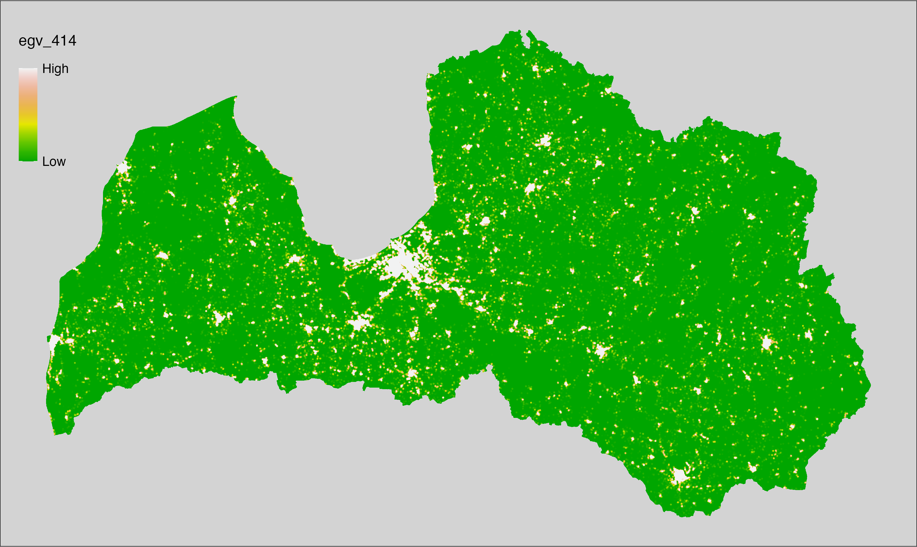
6.415 General_Builtup_r1250
filename: General_Builtup_r1250.tif
layername: egv_415
English name: Fractional cover of Built-Up areas within the 1.25 km landscape
Latvian name: Apbūves platības īpatsvars 1,25 km ainavā
Procedure: The cover fraction within a radius of 1250 m around the analysis grid cell
is calculated as the area-weighted sum of the analysis cells inside
the buffer, using the workflow egvtools::radius_function(). During the calculation of the landscape
metric, inverse distance weighted (power = 2) gap filling on the output is
applied to ensure no missing values at the edges. Then the layer is
rewritten to set its name. Finally, the layer is standardised by
subtracting the arithmetic mean and dividing by the root mean squared error.
Code
# libs ----
if(!require(terra)) {install.packages("terra"); require(terra)}
if(!require(egvtools)) {remotes::install_github("aavotins/egvtools"); require(egvtools)}
# Templates -----
template100=rast("./Templates/TemplateRasters/LV100m_10km.tif")
# radii ----
radius_function(
kvadrati_path = "./Templates/TemplateGrids/tiles/",
radii_path = "./Templates/TemplateGridPoints/tiles/",
tikls100_path = "./Templates/TemplateGrids/tikls100_sauzeme.parquet",
template_path = "./Templates/TemplateRasters/LV100m_10km.tif",
input_layers = c("./RasterGrids_100m/2024/RAW/General_Builtup_cell.tif"),
layer_prefixes = c("General_Builtup"),
output_dir = "./RasterGrids_100m/2024/RAW/",
n_workers = 6,
radii = c("r1250"),
radius_mode = "sparse",
extract_fun = "mean",
fill_missing = TRUE,
IDW_weight = 2,
future_max_size = 40 * 1024^3)
# General_Builtup_r1250.tif egv_415
slanis=rast("./RasterGrids_100m/2024/RAW/General_Builtup_r1250.tif")
names(slanis)="egv_415"
slanis2=project(slanis,template100)
writeRaster(slanis2,
"./RasterGrids_100m/2024/RAW/General_Builtup_r1250.tif",
overwrite=TRUE)
# standardisation ----
if(!require(terra)) {install.packages("terra"); require(terra)}
if(!require(tidyverse)) {install.packages("tidyverse"); require(tidyverse)}
nosaukums="General_Builtup_r1250.tif"
ielasisanas_cels=paste0("./RasterGrids_100m/2024/RAW/",nosaukums)
saglabasanas_cels=paste0("./RasterGrids_100m/2024/Scaled/",nosaukums)
slanis=rast(ielasisanas_cels)
videjais=global(slanis,fun="mean",na.rm=TRUE)
centrets=slanis-videjais[,1]
standartnovirze=terra::global(centrets,fun="rms",na.rm=TRUE)
merogots=centrets/standartnovirze[,1]
writeRaster(merogots,
filename=saglabasanas_cels,
overwrite=TRUE)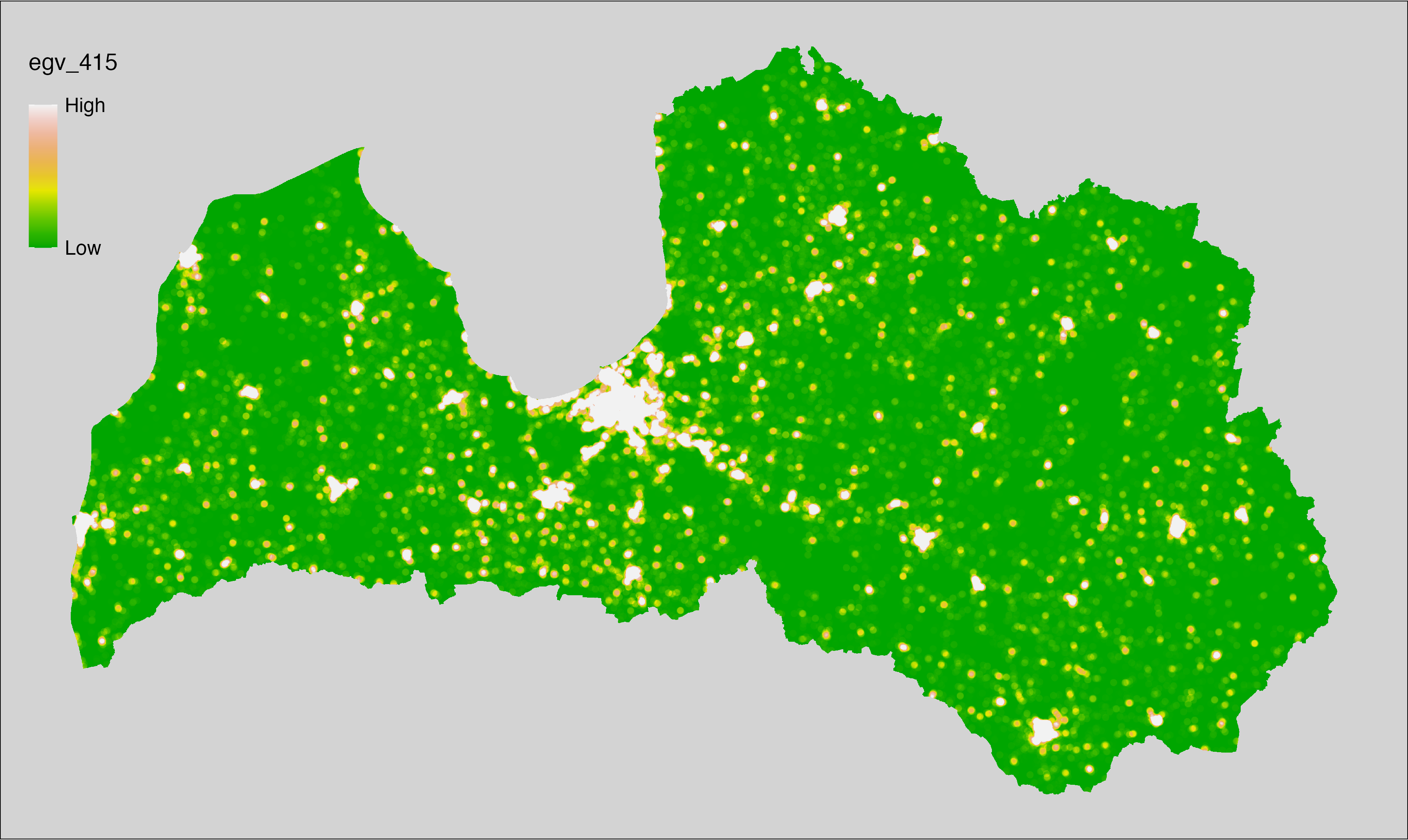
6.416 General_Builtup_r3000
filename: General_Builtup_r3000.tif
layername: egv_416
English name: Fractional cover of Built-Up areas within the 3 km landscape
Latvian name: Apbūves platības īpatsvars 3 km ainavā
Procedure: The cover fraction within a radius of 3000 m around the analysis grid cell
is calculated as the area-weighted sum of the analysis cells inside
the buffer, using the workflow egvtools::radius_function(). During the calculation of the landscape
metric, inverse distance weighted (power = 2) gap filling on the output is
applied to ensure no missing values at the edges. Then the layer is
rewritten to set its name. Finally, the layer is standardised by
subtracting the arithmetic mean and dividing by the root mean squared error.
Code
# libs ----
if(!require(terra)) {install.packages("terra"); require(terra)}
if(!require(egvtools)) {remotes::install_github("aavotins/egvtools"); require(egvtools)}
# Templates -----
template100=rast("./Templates/TemplateRasters/LV100m_10km.tif")
# radii ----
radius_function(
kvadrati_path = "./Templates/TemplateGrids/tiles/",
radii_path = "./Templates/TemplateGridPoints/tiles/",
tikls100_path = "./Templates/TemplateGrids/tikls100_sauzeme.parquet",
template_path = "./Templates/TemplateRasters/LV100m_10km.tif",
input_layers = c("./RasterGrids_100m/2024/RAW/General_Builtup_cell.tif"),
layer_prefixes = c("General_Builtup"),
output_dir = "./RasterGrids_100m/2024/RAW/",
n_workers = 6,
radii = c("r3000"),
radius_mode = "sparse",
extract_fun = "mean",
fill_missing = TRUE,
IDW_weight = 2,
future_max_size = 40 * 1024^3)
# General_Builtup_r3000.tif egv_416
slanis=rast("./RasterGrids_100m/2024/RAW/General_Builtup_r3000.tif")
names(slanis)="egv_416"
slanis2=project(slanis,template100)
writeRaster(slanis2,
"./RasterGrids_100m/2024/RAW/General_Builtup_r3000.tif",
overwrite=TRUE)
# standardisation ----
if(!require(terra)) {install.packages("terra"); require(terra)}
if(!require(tidyverse)) {install.packages("tidyverse"); require(tidyverse)}
nosaukums="General_Builtup_r3000.tif"
ielasisanas_cels=paste0("./RasterGrids_100m/2024/RAW/",nosaukums)
saglabasanas_cels=paste0("./RasterGrids_100m/2024/Scaled/",nosaukums)
slanis=rast(ielasisanas_cels)
videjais=global(slanis,fun="mean",na.rm=TRUE)
centrets=slanis-videjais[,1]
standartnovirze=terra::global(centrets,fun="rms",na.rm=TRUE)
merogots=centrets/standartnovirze[,1]
writeRaster(merogots,
filename=saglabasanas_cels,
overwrite=TRUE)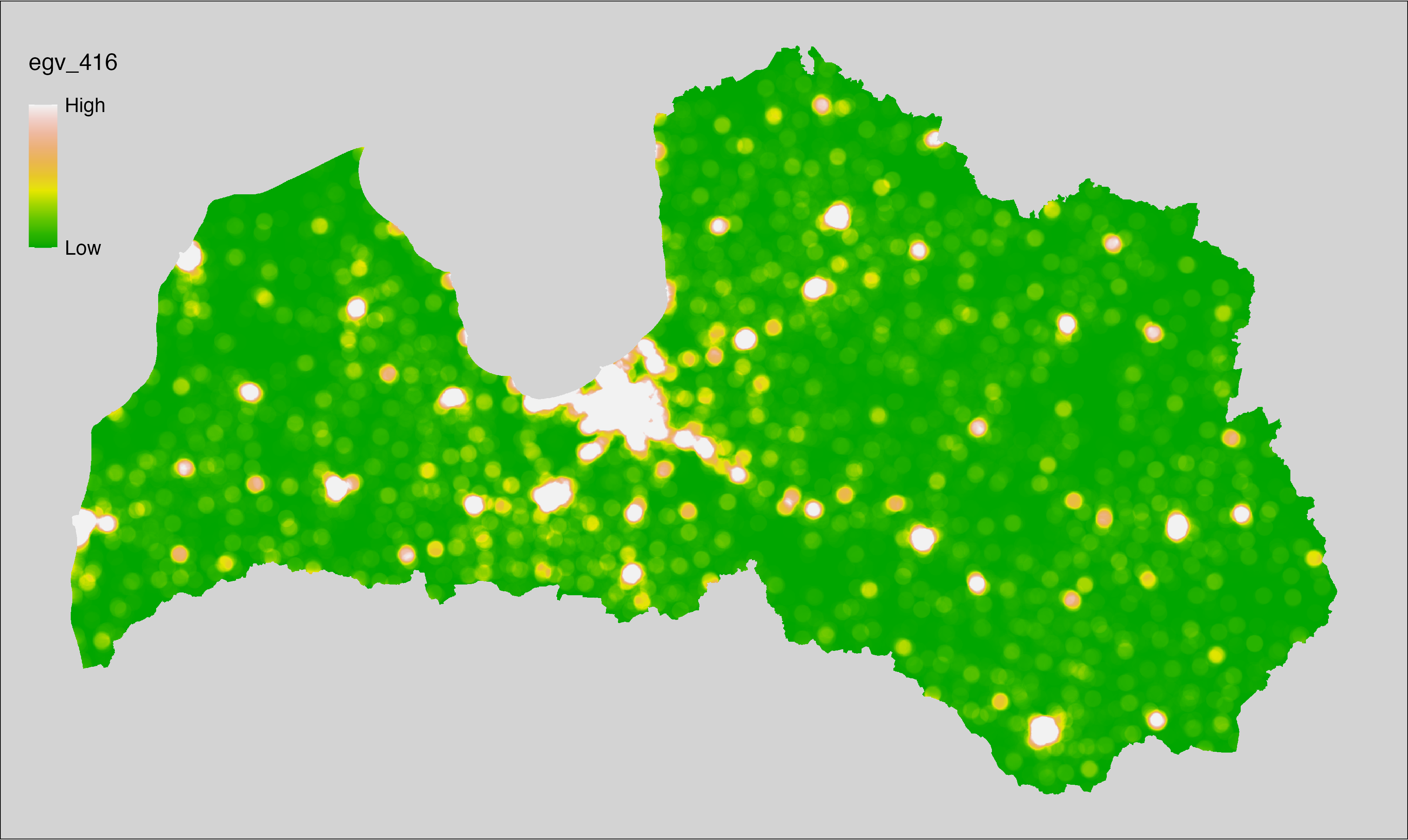
6.417 General_Builtup_r10000
filename: General_Builtup_r10000.tif
layername: egv_417
English name: Fractional cover of Built-Up areas within the 10 km landscape
Latvian name: Apbūves platības īpatsvars 10 km ainavā
Procedure: The cover fraction within a radius of 10000 m around the analysis grid cell
is calculated as the area-weighted sum of the analysis cells inside
the buffer, using the workflow egvtools::radius_function(). During the calculation of the landscape
metric, inverse distance weighted (power = 2) gap filling on the output is
applied to ensure no missing values at the edges. Then the layer is
rewritten to set its name. Finally, the layer is standardised by
subtracting the arithmetic mean and dividing by the root mean squared error.
Code
# libs ----
if(!require(terra)) {install.packages("terra"); require(terra)}
if(!require(egvtools)) {remotes::install_github("aavotins/egvtools"); require(egvtools)}
# Templates -----
template100=rast("./Templates/TemplateRasters/LV100m_10km.tif")
# radii ----
radius_function(
kvadrati_path = "./Templates/TemplateGrids/tiles/",
radii_path = "./Templates/TemplateGridPoints/tiles/",
tikls100_path = "./Templates/TemplateGrids/tikls100_sauzeme.parquet",
template_path = "./Templates/TemplateRasters/LV100m_10km.tif",
input_layers = c("./RasterGrids_100m/2024/RAW/General_Builtup_cell.tif"),
layer_prefixes = c("General_Builtup"),
output_dir = "./RasterGrids_100m/2024/RAW/",
n_workers = 6,
radii = c("r10000"),
radius_mode = "sparse",
extract_fun = "mean",
fill_missing = TRUE,
IDW_weight = 2,
future_max_size = 40 * 1024^3)
# General_Builtup_r10000.tif egv_417
slanis=rast("./RasterGrids_100m/2024/RAW/General_Builtup_r10000.tif")
names(slanis)="egv_417"
slanis2=project(slanis,template100)
writeRaster(slanis2,
"./RasterGrids_100m/2024/RAW/General_Builtup_r10000.tif",
overwrite=TRUE)
# standardisation ----
if(!require(terra)) {install.packages("terra"); require(terra)}
if(!require(tidyverse)) {install.packages("tidyverse"); require(tidyverse)}
nosaukums="General_Builtup_r10000.tif"
ielasisanas_cels=paste0("./RasterGrids_100m/2024/RAW/",nosaukums)
saglabasanas_cels=paste0("./RasterGrids_100m/2024/Scaled/",nosaukums)
slanis=rast(ielasisanas_cels)
videjais=global(slanis,fun="mean",na.rm=TRUE)
centrets=slanis-videjais[,1]
standartnovirze=terra::global(centrets,fun="rms",na.rm=TRUE)
merogots=centrets/standartnovirze[,1]
writeRaster(merogots,
filename=saglabasanas_cels,
overwrite=TRUE)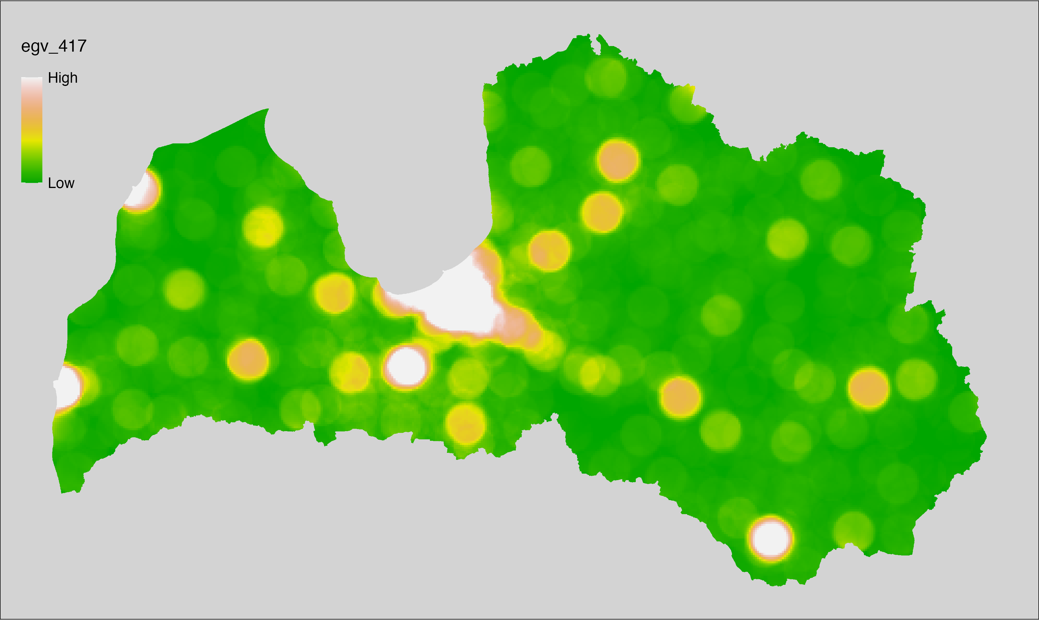
6.418 General_Farmland_cell
filename: General_Farmland_cell.tif
layername: egv_418
English name: Fractional cover of Farmland within the analysis cell (1 ha)
Latvian name: Lauksaimniecībā izmantojamo zemju platības īpatsvars analīzes šūnā (1 ha)
Procedure: First, the farmlands from the Landscape classification are
selected (values between 300 and 400 are reclassified to value 1; all others are set to 0).
The resulting layer
is then aggregated to EGV resolution using the workflow egvtools::input2egv(), which
calculates the arithmetic mean to determine the cover fraction. During
aggregation, inverse distance weighted (power = 2) gap filling on the output is
applied to ensure no missing values at the edges. Finally, the layer is
standardised by subtracting the arithmetic mean and dividing by the root mean squared
error.
Code
# libs ----
if(!require(egvtools)) {remotes::install_github("aavotins/egvtools"); require(egvtools)}
if(!require(terra)) {install.packages("terra"); require(terra)}
if(!require(sf)) {install.packages("sf"); require(sf)}
if(!require(tidyverse)) {install.packages("tidyverse"); require(tidyverse)}
if(!require(sfarrow)) {install.packages("sfarrow"); require(sfarrow)}
if(!require(readxl)) {install.packages("readxl"); require(readxl)}
if(!require(raster)) {install.packages("raster"); require(raster)}
if(!require(fasterize)) {install.packages("fasterize"); require(fasterize)}
# templates ----
template100=rast("./Templates/TemplateRasters/LV100m_10km.tif")
template10=rast("./Templates/TemplateRasters/LV10m_10km.tif")
rastrs10=raster(template10)
nulls10=rast("./Templates/TemplateRasters/nulls_LV10m_10km.tif")
nulls100=rast("./Templates/TemplateRasters/nulls_LV100m_10km.tif")
# simple landscape ----
simple_landscape=rast("RasterGrids_10m/2024/Ainava_vienk_mask.tif")
# General_Farmland_cell.tif egv_418 ----
farmland=ifel(simple_landscape>=300&simple_landscape<400,1,0)
i2e_rez=egvtools::input2egv(input=farmland,
egv_template= "./Templates/TemplateRasters/LV100m_10km.tif",
summary_function = "average",
missing_job = "FillOutput",
outlocation = "./RasterGrids_100m/2024/RAW/",
outfilename = "General_Farmland_cell.tif",
layername = "egv_418",
idw_weight = 2,
plot_gaps = FALSE,plot_final = TRUE)
i2e_rez
rm(farmland)
rm(i2e_rez)
# standardisation ----
if(!require(terra)) {install.packages("terra"); require(terra)}
if(!require(tidyverse)) {install.packages("tidyverse"); require(tidyverse)}
nosaukums="General_Farmland_cell.tif"
ielasisanas_cels=paste0("./RasterGrids_100m/2024/RAW/",nosaukums)
saglabasanas_cels=paste0("./RasterGrids_100m/2024/Scaled/",nosaukums)
slanis=rast(ielasisanas_cels)
videjais=global(slanis,fun="mean",na.rm=TRUE)
centrets=slanis-videjais[,1]
standartnovirze=terra::global(centrets,fun="rms",na.rm=TRUE)
merogots=centrets/standartnovirze[,1]
writeRaster(merogots,
filename=saglabasanas_cels,
overwrite=TRUE)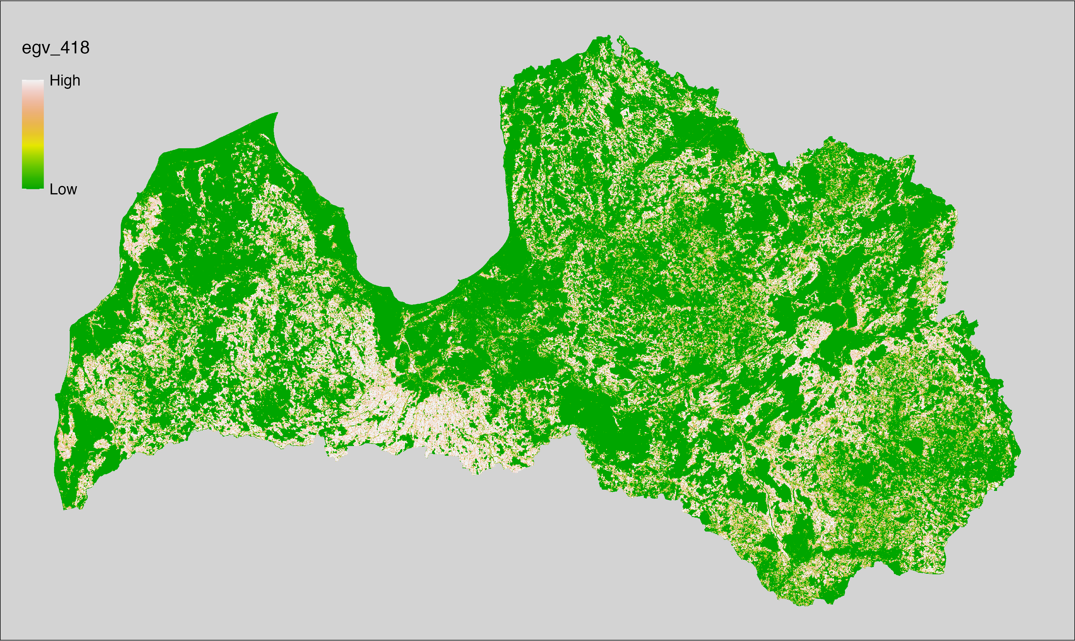
6.419 General_Farmland_r500
filename: General_Farmland_r500.tif
layername: egv_419
English name: Fractional cover of Farmland within the 0.5 km landscape
Latvian name: Lauksaimniecībā izmantojamo zemju platības īpatsvars 0,5 km ainavā
Procedure: The cover fraction within a radius of 500 m around the analysis grid cell is
calculated as the area-weighted sum of the analysis cells inside the
buffer, using the workflow egvtools::radius_function(). During the calculation of the landscape metric,
inverse distance weighted (power = 2) gap filling on the output is applied
to ensure no missing values at the edges. Then the layer is rewritten to set
its name. Finally, the layer is standardised by subtracting the arithmetic
mean and dividing by the root mean squared error.
Code
# libs ----
if(!require(terra)) {install.packages("terra"); require(terra)}
if(!require(egvtools)) {remotes::install_github("aavotins/egvtools"); require(egvtools)}
# Templates -----
template100=rast("./Templates/TemplateRasters/LV100m_10km.tif")
# radii ----
radius_function(
kvadrati_path = "./Templates/TemplateGrids/tiles/",
radii_path = "./Templates/TemplateGridPoints/tiles/",
tikls100_path = "./Templates/TemplateGrids/tikls100_sauzeme.parquet",
template_path = "./Templates/TemplateRasters/LV100m_10km.tif",
input_layers = c("./RasterGrids_100m/2024/RAW/General_Farmland_cell.tif"),
layer_prefixes = c("General_Farmland"),
output_dir = "./RasterGrids_100m/2024/RAW/",
n_workers = 6,
radii = c("r500"),
radius_mode = "sparse",
extract_fun = "mean",
fill_missing = TRUE,
IDW_weight = 2,
future_max_size = 40 * 1024^3)
# General_Farmland_r500.tif egv_419
slanis=rast("./RasterGrids_100m/2024/RAW/General_Farmland_r500.tif")
names(slanis)="egv_419"
slanis2=project(slanis,template100)
writeRaster(slanis2,
"./RasterGrids_100m/2024/RAW/General_Farmland_r500.tif",
overwrite=TRUE)
# standardisation ----
if(!require(terra)) {install.packages("terra"); require(terra)}
if(!require(tidyverse)) {install.packages("tidyverse"); require(tidyverse)}
nosaukums="General_Farmland_r500.tif"
ielasisanas_cels=paste0("./RasterGrids_100m/2024/RAW/",nosaukums)
saglabasanas_cels=paste0("./RasterGrids_100m/2024/Scaled/",nosaukums)
slanis=rast(ielasisanas_cels)
videjais=global(slanis,fun="mean",na.rm=TRUE)
centrets=slanis-videjais[,1]
standartnovirze=terra::global(centrets,fun="rms",na.rm=TRUE)
merogots=centrets/standartnovirze[,1]
writeRaster(merogots,
filename=saglabasanas_cels,
overwrite=TRUE)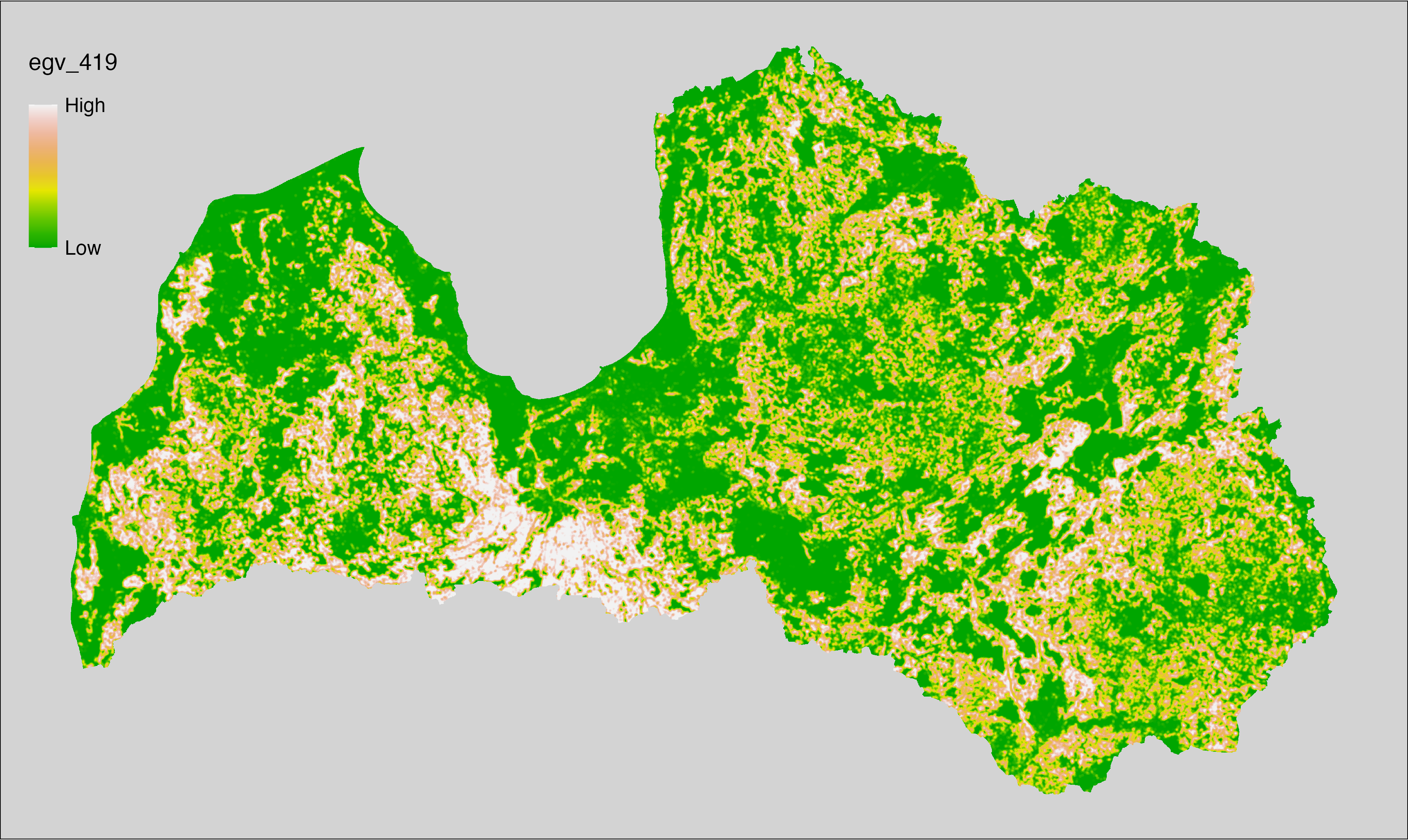
6.420 General_Farmland_r1250
filename: General_Farmland_r1250.tif
layername: egv_420
English name: Fractional cover of Farmland within the 1.25 km landscape
Latvian name: Lauksaimniecībā izmantojamo zemju platības īpatsvars 1,25 km ainavā
Procedure: The cover fraction within a radius of 1250 m around the analysis grid cell
is calculated as the area-weighted sum of the analysis cells inside
the buffer, using the workflow egvtools::radius_function(). During the calculation of the landscape
metric, inverse distance weighted (power = 2) gap filling on the output is
applied to ensure no missing values at the edges. Then the layer is
rewritten to set its name. Finally, the layer is standardised by
subtracting the arithmetic mean and dividing by the root mean squared error.
Code
# libs ----
if(!require(terra)) {install.packages("terra"); require(terra)}
if(!require(egvtools)) {remotes::install_github("aavotins/egvtools"); require(egvtools)}
# Templates -----
template100=rast("./Templates/TemplateRasters/LV100m_10km.tif")
# radii ----
radius_function(
kvadrati_path = "./Templates/TemplateGrids/tiles/",
radii_path = "./Templates/TemplateGridPoints/tiles/",
tikls100_path = "./Templates/TemplateGrids/tikls100_sauzeme.parquet",
template_path = "./Templates/TemplateRasters/LV100m_10km.tif",
input_layers = c("./RasterGrids_100m/2024/RAW/General_Farmland_cell.tif"),
layer_prefixes = c("General_Farmland"),
output_dir = "./RasterGrids_100m/2024/RAW/",
n_workers = 6,
radii = c("r1250"),
radius_mode = "sparse",
extract_fun = "mean",
fill_missing = TRUE,
IDW_weight = 2,
future_max_size = 40 * 1024^3)
# General_Farmland_r1250.tif egv_420
slanis=rast("./RasterGrids_100m/2024/RAW/General_Farmland_r1250.tif")
names(slanis)="egv_420"
slanis2=project(slanis,template100)
writeRaster(slanis2,
"./RasterGrids_100m/2024/RAW/General_Farmland_r1250.tif",
overwrite=TRUE)
# standardisation ----
if(!require(terra)) {install.packages("terra"); require(terra)}
if(!require(tidyverse)) {install.packages("tidyverse"); require(tidyverse)}
nosaukums="General_Farmland_r1250.tif"
ielasisanas_cels=paste0("./RasterGrids_100m/2024/RAW/",nosaukums)
saglabasanas_cels=paste0("./RasterGrids_100m/2024/Scaled/",nosaukums)
slanis=rast(ielasisanas_cels)
videjais=global(slanis,fun="mean",na.rm=TRUE)
centrets=slanis-videjais[,1]
standartnovirze=terra::global(centrets,fun="rms",na.rm=TRUE)
merogots=centrets/standartnovirze[,1]
writeRaster(merogots,
filename=saglabasanas_cels,
overwrite=TRUE)
6.421 General_Farmland_r3000
filename: General_Farmland_r3000.tif
layername: egv_421
English name: Fractional cover of Farmland within the 3 km landscape
Latvian name: Lauksaimniecībā izmantojamo zemju platības īpatsvars 3 km ainavā
Procedure: The cover fraction within a radius of 3000 m around the analysis grid cell
is calculated as the area-weighted sum of the analysis cells inside
the buffer, using the workflow egvtools::radius_function(). During the calculation of the landscape
metric, inverse distance weighted (power = 2) gap filling on the output is
applied to ensure no missing values at the edges. Then the layer is
rewritten to set its name. Finally, the layer is standardised by
subtracting the arithmetic mean and dividing by the root mean squared error.
Code
# libs ----
if(!require(terra)) {install.packages("terra"); require(terra)}
if(!require(egvtools)) {remotes::install_github("aavotins/egvtools"); require(egvtools)}
# Templates -----
template100=rast("./Templates/TemplateRasters/LV100m_10km.tif")
# radii ----
radius_function(
kvadrati_path = "./Templates/TemplateGrids/tiles/",
radii_path = "./Templates/TemplateGridPoints/tiles/",
tikls100_path = "./Templates/TemplateGrids/tikls100_sauzeme.parquet",
template_path = "./Templates/TemplateRasters/LV100m_10km.tif",
input_layers = c("./RasterGrids_100m/2024/RAW/General_Farmland_cell.tif"),
layer_prefixes = c("General_Farmland"),
output_dir = "./RasterGrids_100m/2024/RAW/",
n_workers = 6,
radii = c("r3000"),
radius_mode = "sparse",
extract_fun = "mean",
fill_missing = TRUE,
IDW_weight = 2,
future_max_size = 40 * 1024^3)
# General_Farmland_r3000.tif egv_421
slanis=rast("./RasterGrids_100m/2024/RAW/General_Farmland_r3000.tif")
names(slanis)="egv_421"
slanis2=project(slanis,template100)
writeRaster(slanis2,
"./RasterGrids_100m/2024/RAW/General_Farmland_r3000.tif",
overwrite=TRUE)
# standardisation ----
if(!require(terra)) {install.packages("terra"); require(terra)}
if(!require(tidyverse)) {install.packages("tidyverse"); require(tidyverse)}
nosaukums="General_Farmland_r3000.tif"
ielasisanas_cels=paste0("./RasterGrids_100m/2024/RAW/",nosaukums)
saglabasanas_cels=paste0("./RasterGrids_100m/2024/Scaled/",nosaukums)
slanis=rast(ielasisanas_cels)
videjais=global(slanis,fun="mean",na.rm=TRUE)
centrets=slanis-videjais[,1]
standartnovirze=terra::global(centrets,fun="rms",na.rm=TRUE)
merogots=centrets/standartnovirze[,1]
writeRaster(merogots,
filename=saglabasanas_cels,
overwrite=TRUE)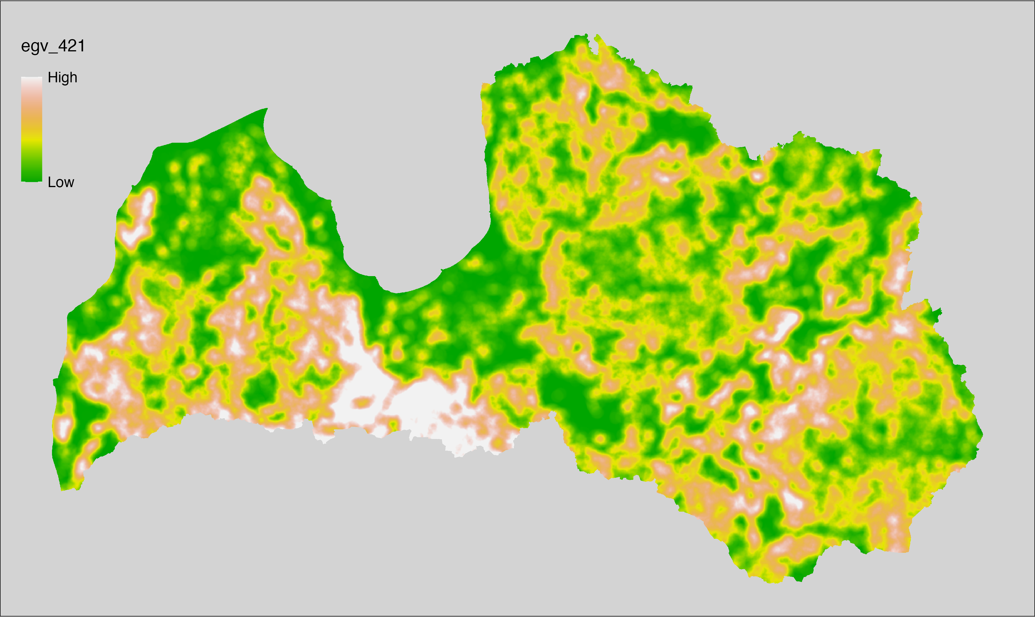
6.422 General_Farmland_r10000
filename: General_Farmland_r10000.tif
layername: egv_422
English name: Fractional cover of Farmland within the 10 km landscape
Latvian name: Lauksaimniecībā izmantojamo zemju platības īpatsvars 10 km ainavā
Procedure: The cover fraction within a radius of 10000 m around the analysis grid cell
is calculated as the area-weighted sum of the analysis cells inside
the buffer, using the workflow egvtools::radius_function(). During the calculation of the landscape
metric, inverse distance weighted (power = 2) gap filling on the output is
applied to ensure no missing values at the edges. Then the layer is
rewritten to set its name. Finally, the layer is standardised by
subtracting the arithmetic mean and dividing by the root mean squared error.
Code
# libs ----
if(!require(terra)) {install.packages("terra"); require(terra)}
if(!require(egvtools)) {remotes::install_github("aavotins/egvtools"); require(egvtools)}
# Templates -----
template100=rast("./Templates/TemplateRasters/LV100m_10km.tif")
# radii ----
radius_function(
kvadrati_path = "./Templates/TemplateGrids/tiles/",
radii_path = "./Templates/TemplateGridPoints/tiles/",
tikls100_path = "./Templates/TemplateGrids/tikls100_sauzeme.parquet",
template_path = "./Templates/TemplateRasters/LV100m_10km.tif",
input_layers = c("./RasterGrids_100m/2024/RAW/General_Farmland_cell.tif"),
layer_prefixes = c("General_Farmland"),
output_dir = "./RasterGrids_100m/2024/RAW/",
n_workers = 6,
radii = c("r10000"),
radius_mode = "sparse",
extract_fun = "mean",
fill_missing = TRUE,
IDW_weight = 2,
future_max_size = 40 * 1024^3)
# General_Farmland_r10000.tif egv_422
slanis=rast("./RasterGrids_100m/2024/RAW/General_Farmland_r10000.tif")
names(slanis)="egv_422"
slanis2=project(slanis,template100)
writeRaster(slanis2,
"./RasterGrids_100m/2024/RAW/General_Farmland_r10000.tif",
overwrite=TRUE)
# standardisation ----
if(!require(terra)) {install.packages("terra"); require(terra)}
if(!require(tidyverse)) {install.packages("tidyverse"); require(tidyverse)}
nosaukums="General_Farmland_r10000.tif"
ielasisanas_cels=paste0("./RasterGrids_100m/2024/RAW/",nosaukums)
saglabasanas_cels=paste0("./RasterGrids_100m/2024/Scaled/",nosaukums)
slanis=rast(ielasisanas_cels)
videjais=global(slanis,fun="mean",na.rm=TRUE)
centrets=slanis-videjais[,1]
standartnovirze=terra::global(centrets,fun="rms",na.rm=TRUE)
merogots=centrets/standartnovirze[,1]
writeRaster(merogots,
filename=saglabasanas_cels,
overwrite=TRUE)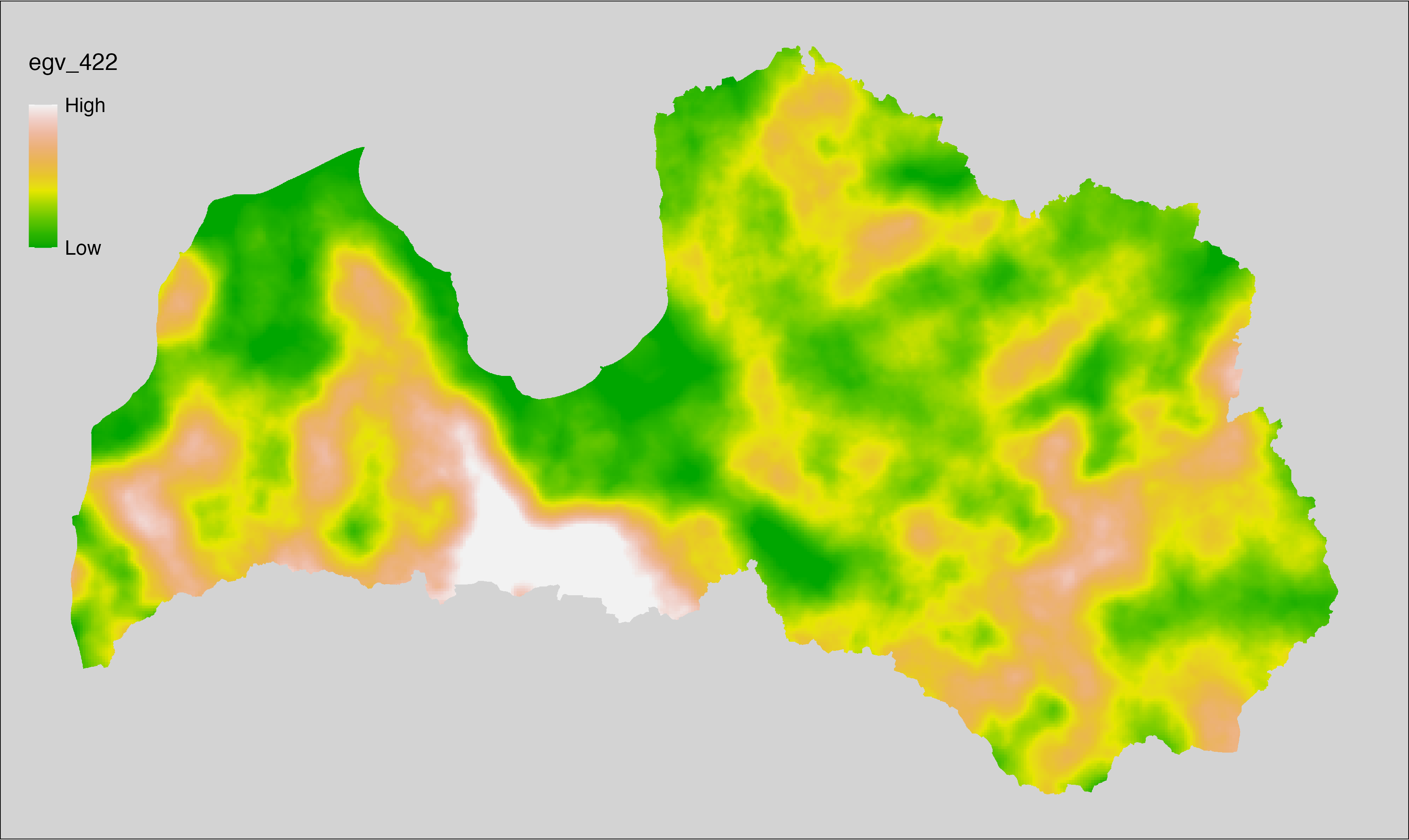
6.423 General_ForestsWithoutInventory_cell
filename: General_ForestsWithoutInventory_cell.tif
layername: egv_423
English name: Fractional cover of Forests Without Inventory within the analysis cell (1 ha)
Latvian name: Netaksēto mežu platības īpatsvars analīzes šūnā (1 ha)
Procedure: First, clearcuts and forest stands from the State Forest Service’s
State Forest Registry are rasterised to match inputs (presence as value 1; NA
elsewhere). Then, from the Landscape classification class 630 is
reclassified to value 1, others to 0). These layers are then combined so that
values 1 from the second layer, where spatially matching NA values in the first
layer and classified as 1; otherwise 0. The resulting layer
is then aggregated to EGV resolution using the workflow egvtools::input2egv(), which
calculates the arithmetic mean to determine the cover fraction. During
aggregation, inverse distance weighted (power = 2) gap filling on the output is
applied to ensure no missing values at the edges. Finally, the layer is
standardised by subtracting the arithmetic mean and dividing by the root mean squared
error.
Code
# libs ----
if(!require(egvtools)) {remotes::install_github("aavotins/egvtools"); require(egvtools)}
if(!require(terra)) {install.packages("terra"); require(terra)}
if(!require(sf)) {install.packages("sf"); require(sf)}
if(!require(tidyverse)) {install.packages("tidyverse"); require(tidyverse)}
if(!require(sfarrow)) {install.packages("sfarrow"); require(sfarrow)}
if(!require(readxl)) {install.packages("readxl"); require(readxl)}
if(!require(raster)) {install.packages("raster"); require(raster)}
if(!require(fasterize)) {install.packages("fasterize"); require(fasterize)}
# templates ----
template100=rast("./Templates/TemplateRasters/LV100m_10km.tif")
template10=rast("./Templates/TemplateRasters/LV10m_10km.tif")
rastrs10=raster(template10)
nulls10=rast("./Templates/TemplateRasters/nulls_LV10m_10km.tif")
nulls100=rast("./Templates/TemplateRasters/nulls_LV100m_10km.tif")
# simple landscape ----
simple_landscape=rast("RasterGrids_10m/2024/Ainava_vienk_mask.tif")
# General_ForestsWithoutInventory_cell.tif egv_423 ----
mvr=st_read_parquet("./Geodata/2024/MVR/nogabali_2024janv.parquet")
tksetie=mvr %>%
mutate(yes=1) %>%
filter(zkat %in% c("10","12","14","16"))
taksetie_r=fasterize(tksetie,rastrs10,field="yes",fun="first")
taksetie_t=rast(taksetie_r)
visi_mezi=ifel(simple_landscape==630,1,0)
netaksetie=ifel(is.na(taksetie_t)&visi_mezi==1,1,0)
plot(netaksetie)
i2e_rez=egvtools::input2egv(input=netaksetie,
egv_template= "./Templates/TemplateRasters/LV100m_10km.tif",
summary_function = "average",
missing_job = "FillOutput",
outlocation = "./RasterGrids_100m/2024/RAW/",
outfilename = "General_ForestsWithoutInventory_cell.tif",
layername = "egv_423",
idw_weight = 2,
plot_gaps = FALSE,plot_final = TRUE)
i2e_rez
rm(netaksetie)
rm(i2e_rez)
rm(mvr)
rm(tksetie)
rm(taksetie_r)
rm(taksetie_t)
rm(visi_mezi)
# standardisation ----
if(!require(terra)) {install.packages("terra"); require(terra)}
if(!require(tidyverse)) {install.packages("tidyverse"); require(tidyverse)}
nosaukums="General_ForestsWithoutInventory_cell.tif"
ielasisanas_cels=paste0("./RasterGrids_100m/2024/RAW/",nosaukums)
saglabasanas_cels=paste0("./RasterGrids_100m/2024/Scaled/",nosaukums)
slanis=rast(ielasisanas_cels)
videjais=global(slanis,fun="mean",na.rm=TRUE)
centrets=slanis-videjais[,1]
standartnovirze=terra::global(centrets,fun="rms",na.rm=TRUE)
merogots=centrets/standartnovirze[,1]
writeRaster(merogots,
filename=saglabasanas_cels,
overwrite=TRUE)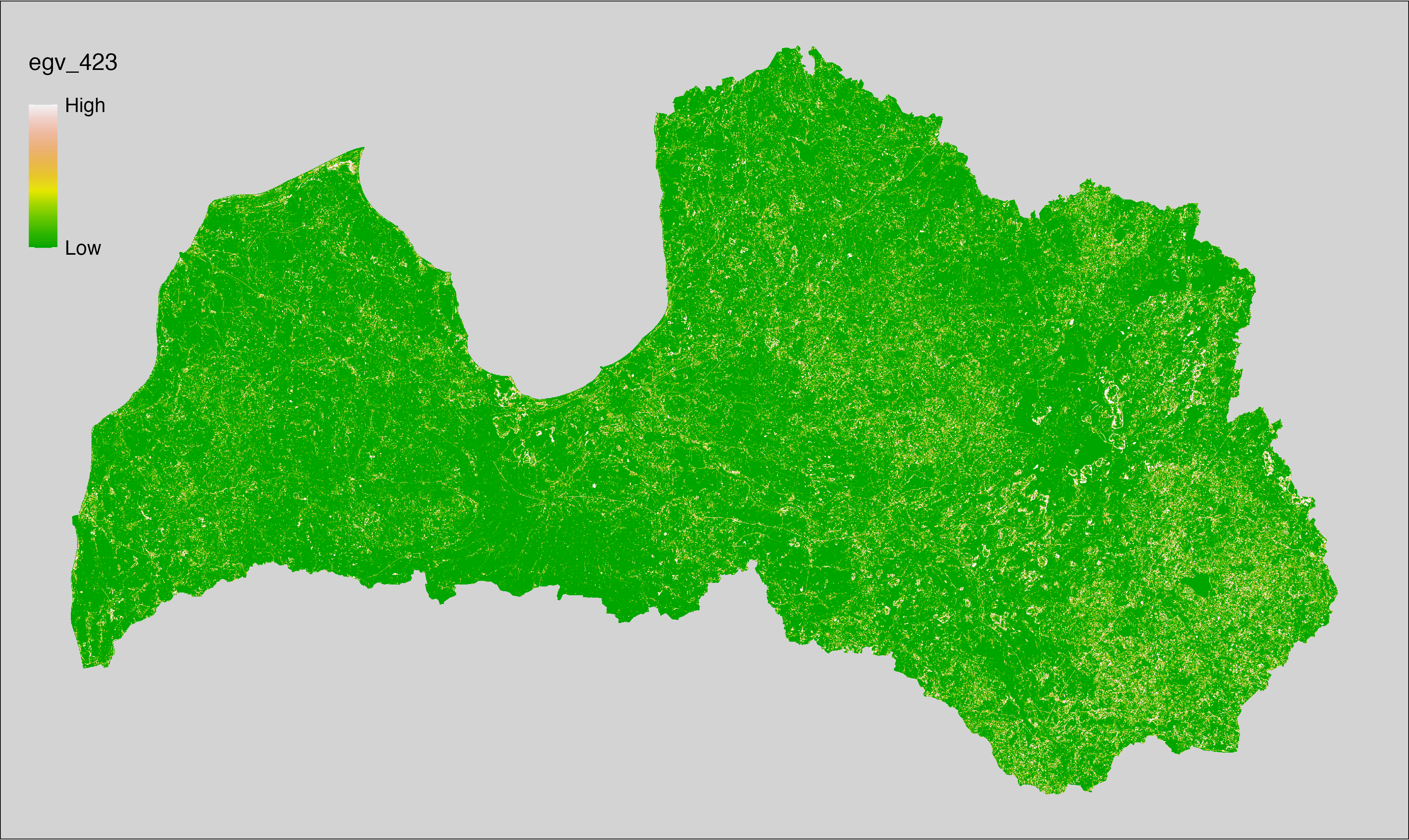
6.424 General_ForestsWithoutInventory_r500
filename: General_ForestsWithoutInventory_r500.tif
layername: egv_424
English name: Fractional cover of Forests Without Inventory within the 0.5 km landscape
Latvian name: Netaksēto mežu platības īpatsvars 0,5 km ainavā
Procedure: The cover fraction within a radius of 500 m around the analysis grid cell is
calculated as the area-weighted sum of the analysis cells inside the
buffer, using the workflow egvtools::radius_function(). During the calculation of the landscape metric,
inverse distance weighted (power = 2) gap filling on the output is applied
to ensure no missing values at the edges. Then the layer is rewritten to set
its name. Finally, the layer is standardised by subtracting the arithmetic
mean and dividing by the root mean squared error.
Code
# libs ----
if(!require(terra)) {install.packages("terra"); require(terra)}
if(!require(egvtools)) {remotes::install_github("aavotins/egvtools"); require(egvtools)}
# Templates -----
template100=rast("./Templates/TemplateRasters/LV100m_10km.tif")
# radii ----
radius_function(
kvadrati_path = "./Templates/TemplateGrids/tiles/",
radii_path = "./Templates/TemplateGridPoints/tiles/",
tikls100_path = "./Templates/TemplateGrids/tikls100_sauzeme.parquet",
template_path = "./Templates/TemplateRasters/LV100m_10km.tif",
input_layers = c("./RasterGrids_100m/2024/RAW/General_ForestsWithoutInventory_cell.tif"),
layer_prefixes = c("General_ForestsWithoutInventory"),
output_dir = "./RasterGrids_100m/2024/RAW/",
n_workers = 6,
radii = c("r500"),
radius_mode = "sparse",
extract_fun = "mean",
fill_missing = TRUE,
IDW_weight = 2,
future_max_size = 40 * 1024^3)
# General_ForestsWithoutInventory_r500.tif egv_424
slanis=rast("./RasterGrids_100m/2024/RAW/General_ForestsWithoutInventory_r500.tif")
names(slanis)="egv_424"
slanis2=project(slanis,template100)
writeRaster(slanis2,
"./RasterGrids_100m/2024/RAW/General_ForestsWithoutInventory_r500.tif",
overwrite=TRUE)
# standardisation ----
if(!require(terra)) {install.packages("terra"); require(terra)}
if(!require(tidyverse)) {install.packages("tidyverse"); require(tidyverse)}
nosaukums="General_ForestsWithoutInventory_r500.tif"
ielasisanas_cels=paste0("./RasterGrids_100m/2024/RAW/",nosaukums)
saglabasanas_cels=paste0("./RasterGrids_100m/2024/Scaled/",nosaukums)
slanis=rast(ielasisanas_cels)
videjais=global(slanis,fun="mean",na.rm=TRUE)
centrets=slanis-videjais[,1]
standartnovirze=terra::global(centrets,fun="rms",na.rm=TRUE)
merogots=centrets/standartnovirze[,1]
writeRaster(merogots,
filename=saglabasanas_cels,
overwrite=TRUE)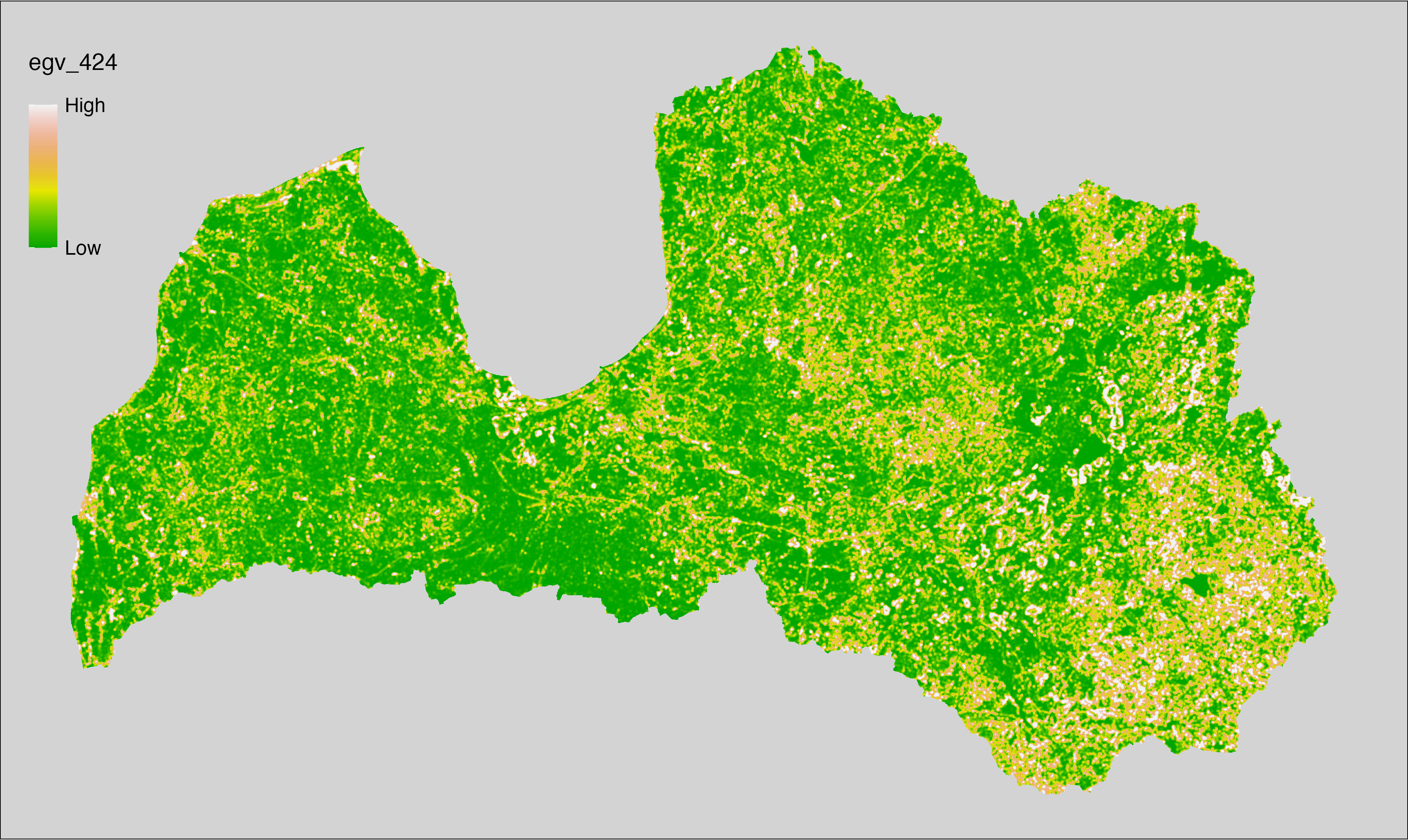
6.425 General_ForestsWithoutInventory_r1250
filename: General_ForestsWithoutInventory_r1250.tif
layername: egv_425
English name: Fractional cover of Forests Without Inventory within the 1.25 km landscape
Latvian name: Netaksēto mežu platības īpatsvars 1,25 km ainavā
Procedure: The cover fraction within a radius of 1250 m around the analysis grid cell
is calculated as the area-weighted sum of the analysis cells inside
the buffer, using the workflow egvtools::radius_function(). During the calculation of the landscape
metric, inverse distance weighted (power = 2) gap filling on the output is
applied to ensure no missing values at the edges. Then the layer is
rewritten to set its name. Finally, the layer is standardised by
subtracting the arithmetic mean and dividing by the root mean squared error.
Code
# libs ----
if(!require(terra)) {install.packages("terra"); require(terra)}
if(!require(egvtools)) {remotes::install_github("aavotins/egvtools"); require(egvtools)}
# Templates -----
template100=rast("./Templates/TemplateRasters/LV100m_10km.tif")
# radii ----
radius_function(
kvadrati_path = "./Templates/TemplateGrids/tiles/",
radii_path = "./Templates/TemplateGridPoints/tiles/",
tikls100_path = "./Templates/TemplateGrids/tikls100_sauzeme.parquet",
template_path = "./Templates/TemplateRasters/LV100m_10km.tif",
input_layers = c("./RasterGrids_100m/2024/RAW/General_ForestsWithoutInventory_cell.tif"),
layer_prefixes = c("General_ForestsWithoutInventory"),
output_dir = "./RasterGrids_100m/2024/RAW/",
n_workers = 6,
radii = c("r1250"),
radius_mode = "sparse",
extract_fun = "mean",
fill_missing = TRUE,
IDW_weight = 2,
future_max_size = 40 * 1024^3)
# General_ForestsWithoutInventory_r1250.tif egv_425
slanis=rast("./RasterGrids_100m/2024/RAW/General_ForestsWithoutInventory_r1250.tif")
names(slanis)="egv_425"
slanis2=project(slanis,template100)
writeRaster(slanis2,
"./RasterGrids_100m/2024/RAW/General_ForestsWithoutInventory_r1250.tif",
overwrite=TRUE)
# standardisation ----
if(!require(terra)) {install.packages("terra"); require(terra)}
if(!require(tidyverse)) {install.packages("tidyverse"); require(tidyverse)}
nosaukums="General_ForestsWithoutInventory_r1250.tif"
ielasisanas_cels=paste0("./RasterGrids_100m/2024/RAW/",nosaukums)
saglabasanas_cels=paste0("./RasterGrids_100m/2024/Scaled/",nosaukums)
slanis=rast(ielasisanas_cels)
videjais=global(slanis,fun="mean",na.rm=TRUE)
centrets=slanis-videjais[,1]
standartnovirze=terra::global(centrets,fun="rms",na.rm=TRUE)
merogots=centrets/standartnovirze[,1]
writeRaster(merogots,
filename=saglabasanas_cels,
overwrite=TRUE)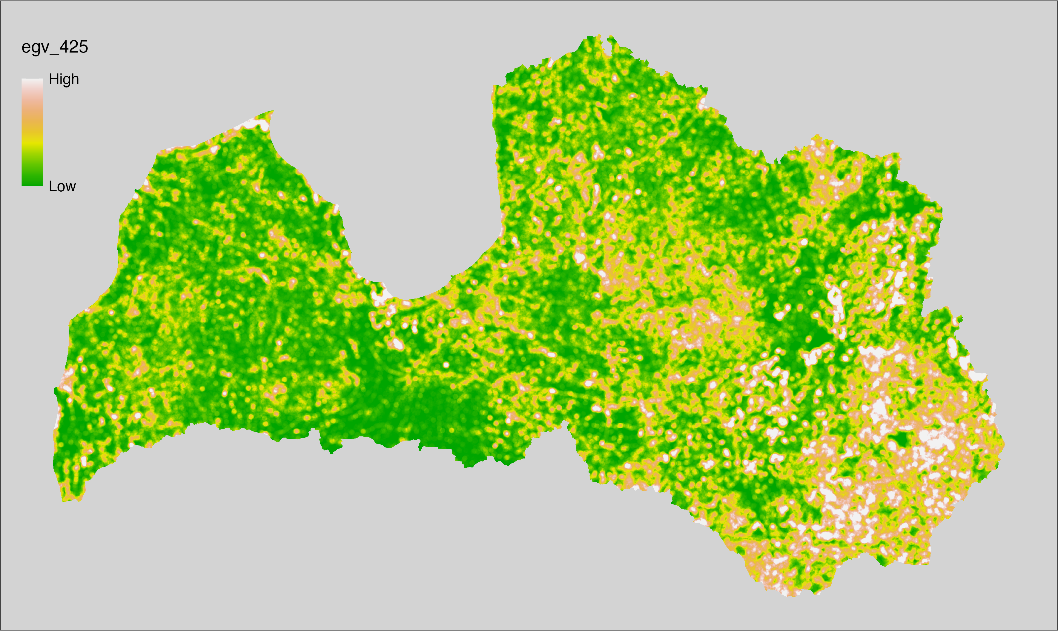
6.426 General_ForestsWithoutInventory_r3000
filename: General_ForestsWithoutInventory_r3000.tif
layername: egv_426
English name: Fractional cover of Forests Without Inventory within the 3 km landscape
Latvian name: Netaksēto mežu platības īpatsvars 3 km ainavā
Procedure: The cover fraction within a radius of 3000 m around the analysis grid cell
is calculated as the area-weighted sum of the analysis cells inside
the buffer, using the workflow egvtools::radius_function(). During the calculation of the landscape
metric, inverse distance weighted (power = 2) gap filling on the output is
applied to ensure no missing values at the edges. Then the layer is
rewritten to set its name. Finally, the layer is standardised by
subtracting the arithmetic mean and dividing by the root mean squared error.
Code
# libs ----
if(!require(terra)) {install.packages("terra"); require(terra)}
if(!require(egvtools)) {remotes::install_github("aavotins/egvtools"); require(egvtools)}
# Templates -----
template100=rast("./Templates/TemplateRasters/LV100m_10km.tif")
# radii ----
radius_function(
kvadrati_path = "./Templates/TemplateGrids/tiles/",
radii_path = "./Templates/TemplateGridPoints/tiles/",
tikls100_path = "./Templates/TemplateGrids/tikls100_sauzeme.parquet",
template_path = "./Templates/TemplateRasters/LV100m_10km.tif",
input_layers = c("./RasterGrids_100m/2024/RAW/General_ForestsWithoutInventory_cell.tif"),
layer_prefixes = c("General_ForestsWithoutInventory"),
output_dir = "./RasterGrids_100m/2024/RAW/",
n_workers = 6,
radii = c("r3000"),
radius_mode = "sparse",
extract_fun = "mean",
fill_missing = TRUE,
IDW_weight = 2,
future_max_size = 40 * 1024^3)
# General_ForestsWithoutInventory_r3000.tif egv_426
slanis=rast("./RasterGrids_100m/2024/RAW/General_ForestsWithoutInventory_r3000.tif")
names(slanis)="egv_426"
slanis2=project(slanis,template100)
writeRaster(slanis2,
"./RasterGrids_100m/2024/RAW/General_ForestsWithoutInventory_r3000.tif",
overwrite=TRUE)
# standardisation ----
if(!require(terra)) {install.packages("terra"); require(terra)}
if(!require(tidyverse)) {install.packages("tidyverse"); require(tidyverse)}
nosaukums="General_ForestsWithoutInventory_r3000.tif"
ielasisanas_cels=paste0("./RasterGrids_100m/2024/RAW/",nosaukums)
saglabasanas_cels=paste0("./RasterGrids_100m/2024/Scaled/",nosaukums)
slanis=rast(ielasisanas_cels)
videjais=global(slanis,fun="mean",na.rm=TRUE)
centrets=slanis-videjais[,1]
standartnovirze=terra::global(centrets,fun="rms",na.rm=TRUE)
merogots=centrets/standartnovirze[,1]
writeRaster(merogots,
filename=saglabasanas_cels,
overwrite=TRUE)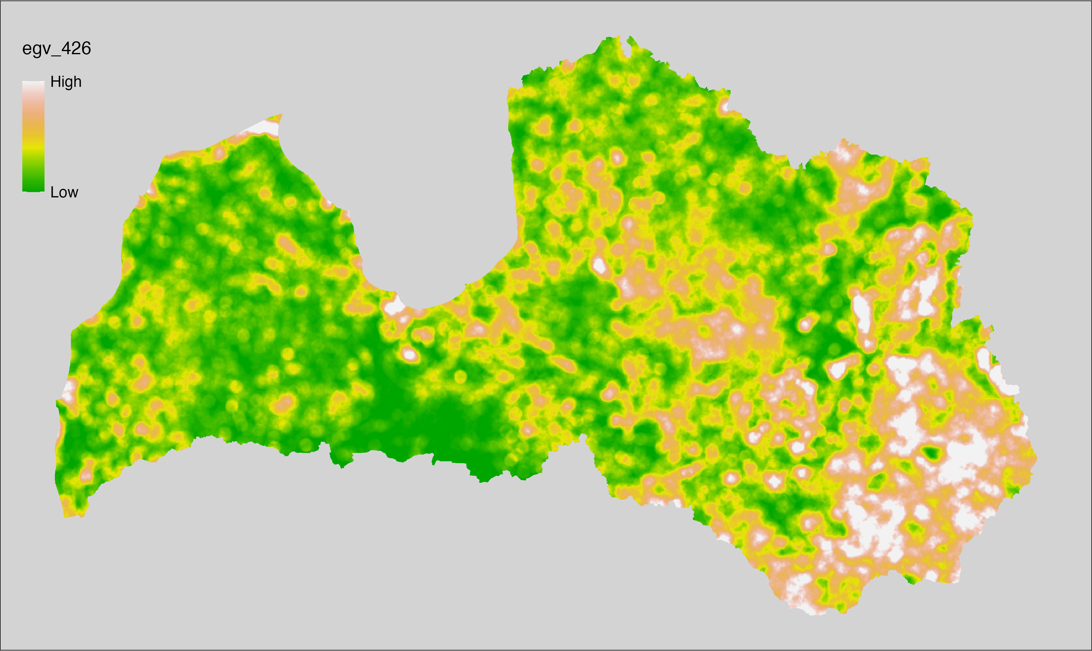
6.427 General_ForestsWithoutInventory_r10000
filename: General_ForestsWithoutInventory_r10000.tif
layername: egv_427
English name: Fractional cover of Forests Without Inventory within the 10 km landscape
Latvian name: Netaksēto mežu platības īpatsvars 10 km ainavā
Procedure: The cover fraction within a radius of 10000 m around the analysis grid cell
is calculated as the area-weighted sum of the analysis cells inside
the buffer, using the workflow egvtools::radius_function(). During the calculation of the landscape
metric, inverse distance weighted (power = 2) gap filling on the output is
applied to ensure no missing values at the edges. Then the layer is
rewritten to set its name. Finally, the layer is standardised by
subtracting the arithmetic mean and dividing by the root mean squared error.
Code
# libs ----
if(!require(terra)) {install.packages("terra"); require(terra)}
if(!require(egvtools)) {remotes::install_github("aavotins/egvtools"); require(egvtools)}
# Templates -----
template100=rast("./Templates/TemplateRasters/LV100m_10km.tif")
# radii ----
radius_function(
kvadrati_path = "./Templates/TemplateGrids/tiles/",
radii_path = "./Templates/TemplateGridPoints/tiles/",
tikls100_path = "./Templates/TemplateGrids/tikls100_sauzeme.parquet",
template_path = "./Templates/TemplateRasters/LV100m_10km.tif",
input_layers = c("./RasterGrids_100m/2024/RAW/General_ForestsWithoutInventory_cell.tif"),
layer_prefixes = c("General_ForestsWithoutInventory"),
output_dir = "./RasterGrids_100m/2024/RAW/",
n_workers = 6,
radii = c("r10000"),
radius_mode = "sparse",
extract_fun = "mean",
fill_missing = TRUE,
IDW_weight = 2,
future_max_size = 40 * 1024^3)
# General_ForestsWithoutInventory_r10000.tif egv_427
slanis=rast("./RasterGrids_100m/2024/RAW/General_ForestsWithoutInventory_r10000.tif")
names(slanis)="egv_427"
slanis2=project(slanis,template100)
writeRaster(slanis2,
"./RasterGrids_100m/2024/RAW/General_ForestsWithoutInventory_r10000.tif",
overwrite=TRUE)
# standardisation ----
if(!require(terra)) {install.packages("terra"); require(terra)}
if(!require(tidyverse)) {install.packages("tidyverse"); require(tidyverse)}
nosaukums="General_ForestsWithoutInventory_r10000.tif"
ielasisanas_cels=paste0("./RasterGrids_100m/2024/RAW/",nosaukums)
saglabasanas_cels=paste0("./RasterGrids_100m/2024/Scaled/",nosaukums)
slanis=rast(ielasisanas_cels)
videjais=global(slanis,fun="mean",na.rm=TRUE)
centrets=slanis-videjais[,1]
standartnovirze=terra::global(centrets,fun="rms",na.rm=TRUE)
merogots=centrets/standartnovirze[,1]
writeRaster(merogots,
filename=saglabasanas_cels,
overwrite=TRUE)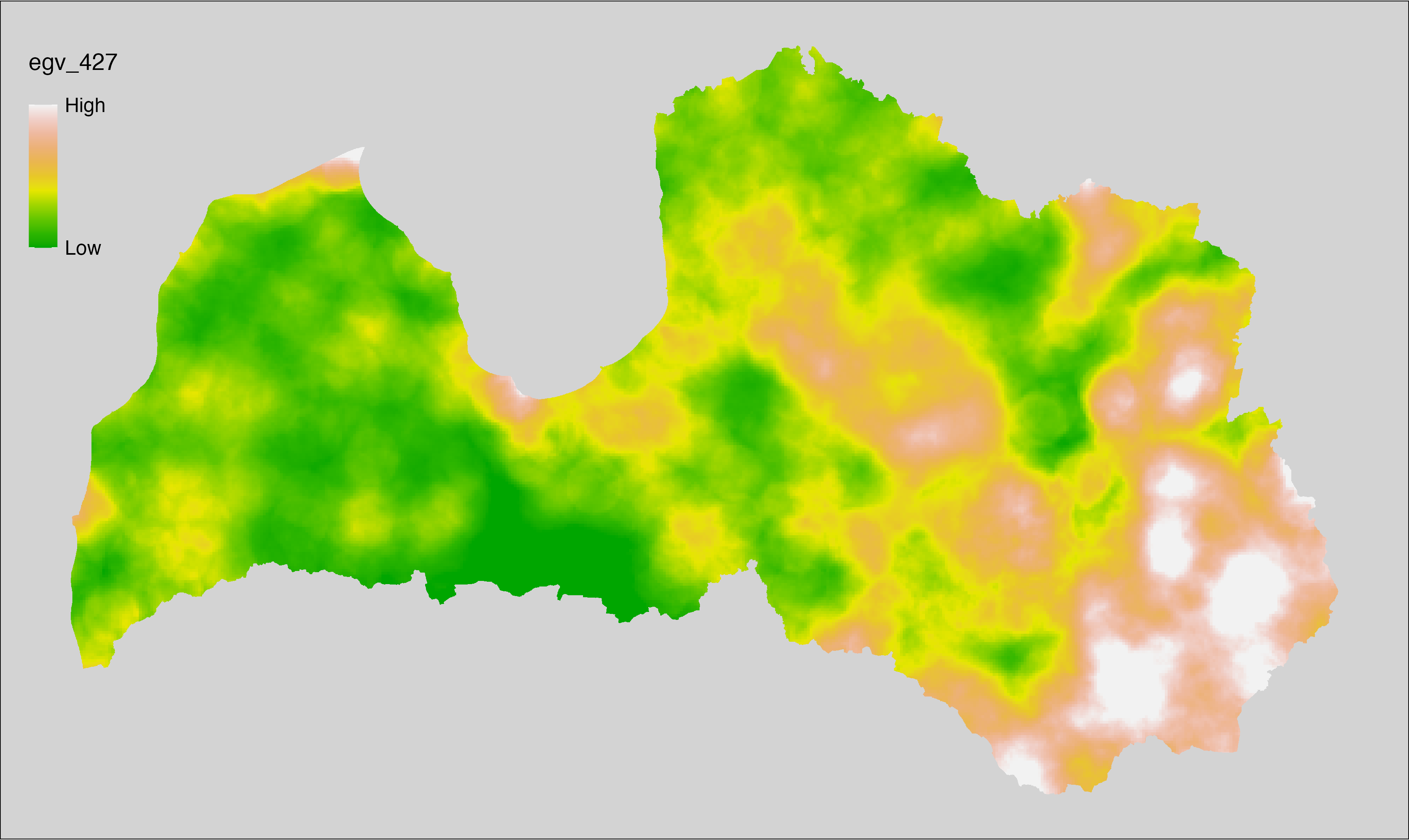
6.428 General_GardensOrchards_cell
filename: General_GardensOrchards_cell.tif
layername: egv_428
English name: Fractional cover of Allotment gardens, Orchards within the analysis cell (1 ha)
Latvian name: Vasarnīcu kompleksu un augļudārzu platības īpatsvars analīzes šūnā (1 ha)
Procedure: First, the allotment gardens and orchards from the Landscape
classification are selected (values between 400 and 500 are
reclassified to value 1; all others are set to 0). The resulting layer
is then aggregated to EGV resolution using the workflow egvtools::input2egv(), which
calculates the arithmetic mean to determine the cover fraction. During
aggregation, inverse distance weighted (power = 2) gap filling on the output is
applied to ensure no missing values at the edges. Finally, the layer is
standardised by subtracting the arithmetic mean and dividing by the root mean squared
error.
Code
# libs ----
if(!require(egvtools)) {remotes::install_github("aavotins/egvtools"); require(egvtools)}
if(!require(terra)) {install.packages("terra"); require(terra)}
if(!require(sf)) {install.packages("sf"); require(sf)}
if(!require(tidyverse)) {install.packages("tidyverse"); require(tidyverse)}
if(!require(sfarrow)) {install.packages("sfarrow"); require(sfarrow)}
if(!require(readxl)) {install.packages("readxl"); require(readxl)}
if(!require(raster)) {install.packages("raster"); require(raster)}
if(!require(fasterize)) {install.packages("fasterize"); require(fasterize)}
# templates ----
template100=rast("./Templates/TemplateRasters/LV100m_10km.tif")
template10=rast("./Templates/TemplateRasters/LV10m_10km.tif")
rastrs10=raster(template10)
nulls10=rast("./Templates/TemplateRasters/nulls_LV10m_10km.tif")
nulls100=rast("./Templates/TemplateRasters/nulls_LV100m_10km.tif")
# simple landscape ----
simple_landscape=rast("RasterGrids_10m/2024/Ainava_vienk_mask.tif")
# General_GardensOrchards_cell.tif egv_428 ----
parejie=ifel(simple_landscape>=400&simple_landscape<500,1,0)
i2e_rez=egvtools::input2egv(input=parejie,
egv_template= "./Templates/TemplateRasters/LV100m_10km.tif",
summary_function = "average",
missing_job = "FillOutput",
outlocation = "./RasterGrids_100m/2024/RAW/",
outfilename = "General_GardensOrchards_cell.tif",
layername = "egv_428",
idw_weight = 2,
plot_gaps = FALSE,plot_final = TRUE)
i2e_rez
rm(parejie)
rm(i2e_rez)
# standardisation ----
if(!require(terra)) {install.packages("terra"); require(terra)}
if(!require(tidyverse)) {install.packages("tidyverse"); require(tidyverse)}
nosaukums="General_GardensOrchards_cell.tif"
ielasisanas_cels=paste0("./RasterGrids_100m/2024/RAW/",nosaukums)
saglabasanas_cels=paste0("./RasterGrids_100m/2024/Scaled/",nosaukums)
slanis=rast(ielasisanas_cels)
videjais=global(slanis,fun="mean",na.rm=TRUE)
centrets=slanis-videjais[,1]
standartnovirze=terra::global(centrets,fun="rms",na.rm=TRUE)
merogots=centrets/standartnovirze[,1]
writeRaster(merogots,
filename=saglabasanas_cels,
overwrite=TRUE)
6.429 General_GardensOrchards_r500
filename: General_GardensOrchards_r500.tif
layername: egv_429
English name: Fractional cover of Allotment gardens, Orchards within the 0.5 km landscape
Latvian name: Vasarnīcu kompleksu un augļudārzu platības īpatsvars 0,5 km ainavā
Procedure: The cover fraction within a radius of 500 m around the analysis grid cell is
calculated as the area-weighted sum of the analysis cells inside the
buffer, using the workflow egvtools::radius_function(). During the calculation of the landscape metric,
inverse distance weighted (power = 2) gap filling on the output is applied
to ensure no missing values at the edges. Then the layer is rewritten to set
its name. Finally, the layer is standardised by subtracting the arithmetic
mean and dividing by the root mean squared error.
Code
# libs ----
if(!require(terra)) {install.packages("terra"); require(terra)}
if(!require(egvtools)) {remotes::install_github("aavotins/egvtools"); require(egvtools)}
# Templates -----
template100=rast("./Templates/TemplateRasters/LV100m_10km.tif")
# radii ----
radius_function(
kvadrati_path = "./Templates/TemplateGrids/tiles/",
radii_path = "./Templates/TemplateGridPoints/tiles/",
tikls100_path = "./Templates/TemplateGrids/tikls100_sauzeme.parquet",
template_path = "./Templates/TemplateRasters/LV100m_10km.tif",
input_layers = c("./RasterGrids_100m/2024/RAW/General_GardensOrchards_cell.tif"),
layer_prefixes = c("General_GardensOrchards"),
output_dir = "./RasterGrids_100m/2024/RAW/",
n_workers = 6,
radii = c("r500"),
radius_mode = "sparse",
extract_fun = "mean",
fill_missing = TRUE,
IDW_weight = 2,
future_max_size = 40 * 1024^3)
# General_GardensOrchards_r500.tif egv_429
slanis=rast("./RasterGrids_100m/2024/RAW/General_GardensOrchards_r500.tif")
names(slanis)="egv_429"
slanis2=project(slanis,template100)
writeRaster(slanis2,
"./RasterGrids_100m/2024/RAW/General_GardensOrchards_r500.tif",
overwrite=TRUE)
# standardisation ----
if(!require(terra)) {install.packages("terra"); require(terra)}
if(!require(tidyverse)) {install.packages("tidyverse"); require(tidyverse)}
nosaukums="General_GardensOrchards_r500.tif"
ielasisanas_cels=paste0("./RasterGrids_100m/2024/RAW/",nosaukums)
saglabasanas_cels=paste0("./RasterGrids_100m/2024/Scaled/",nosaukums)
slanis=rast(ielasisanas_cels)
videjais=global(slanis,fun="mean",na.rm=TRUE)
centrets=slanis-videjais[,1]
standartnovirze=terra::global(centrets,fun="rms",na.rm=TRUE)
merogots=centrets/standartnovirze[,1]
writeRaster(merogots,
filename=saglabasanas_cels,
overwrite=TRUE)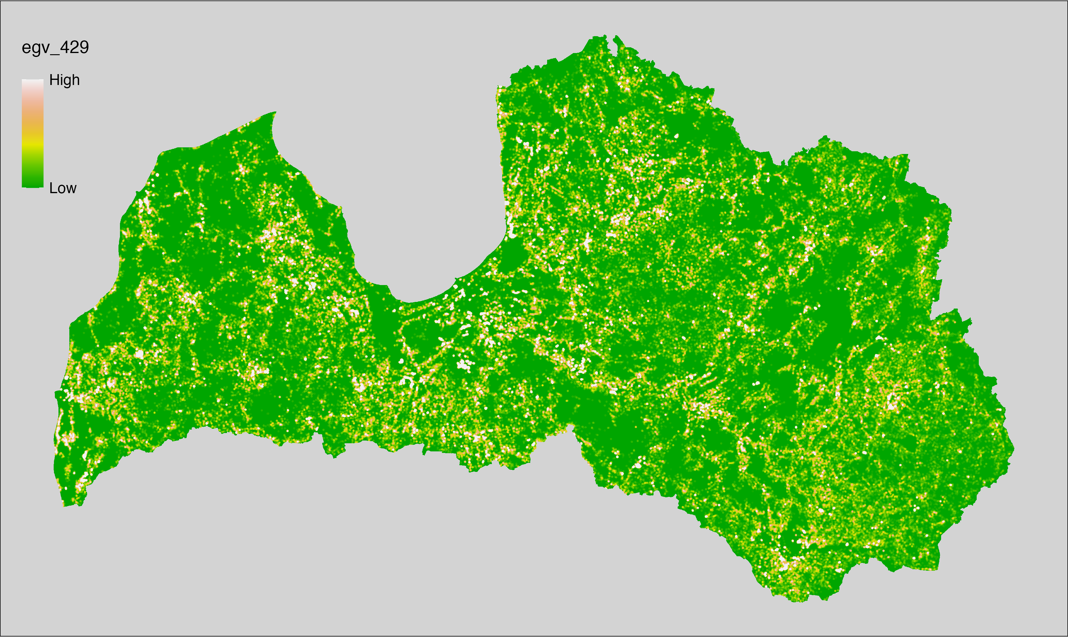
6.430 General_GardensOrchards_r1250
filename: General_GardensOrchards_r1250.tif
layername: egv_430
English name: Fractional cover of Allotment gardens, Orchards within the 1.25 km landscape
Latvian name: Vasarnīcu kompleksu un augļudārzu platības īpatsvars 1,25 km ainavā
Procedure: The cover fraction within a radius of 1250 m around the analysis grid cell
is calculated as the area-weighted sum of the analysis cells inside
the buffer, using the workflow egvtools::radius_function(). During the calculation of the landscape
metric, inverse distance weighted (power = 2) gap filling on the output is
applied to ensure no missing values at the edges. Then the layer is
rewritten to set its name. Finally, the layer is standardised by
subtracting the arithmetic mean and dividing by the root mean squared error.
Code
# libs ----
if(!require(terra)) {install.packages("terra"); require(terra)}
if(!require(egvtools)) {remotes::install_github("aavotins/egvtools"); require(egvtools)}
# Templates -----
template100=rast("./Templates/TemplateRasters/LV100m_10km.tif")
# radii ----
radius_function(
kvadrati_path = "./Templates/TemplateGrids/tiles/",
radii_path = "./Templates/TemplateGridPoints/tiles/",
tikls100_path = "./Templates/TemplateGrids/tikls100_sauzeme.parquet",
template_path = "./Templates/TemplateRasters/LV100m_10km.tif",
input_layers = c("./RasterGrids_100m/2024/RAW/General_GardensOrchards_cell.tif"),
layer_prefixes = c("General_GardensOrchards"),
output_dir = "./RasterGrids_100m/2024/RAW/",
n_workers = 6,
radii = c("r1250"),
radius_mode = "sparse",
extract_fun = "mean",
fill_missing = TRUE,
IDW_weight = 2,
future_max_size = 40 * 1024^3)
# General_GardensOrchards_r1250.tif egv_430
slanis=rast("./RasterGrids_100m/2024/RAW/General_GardensOrchards_r1250.tif")
names(slanis)="egv_430"
slanis2=project(slanis,template100)
writeRaster(slanis2,
"./RasterGrids_100m/2024/RAW/General_GardensOrchards_r1250.tif",
overwrite=TRUE)
# standardisation ----
if(!require(terra)) {install.packages("terra"); require(terra)}
if(!require(tidyverse)) {install.packages("tidyverse"); require(tidyverse)}
nosaukums="General_GardensOrchards_r1250.tif"
ielasisanas_cels=paste0("./RasterGrids_100m/2024/RAW/",nosaukums)
saglabasanas_cels=paste0("./RasterGrids_100m/2024/Scaled/",nosaukums)
slanis=rast(ielasisanas_cels)
videjais=global(slanis,fun="mean",na.rm=TRUE)
centrets=slanis-videjais[,1]
standartnovirze=terra::global(centrets,fun="rms",na.rm=TRUE)
merogots=centrets/standartnovirze[,1]
writeRaster(merogots,
filename=saglabasanas_cels,
overwrite=TRUE)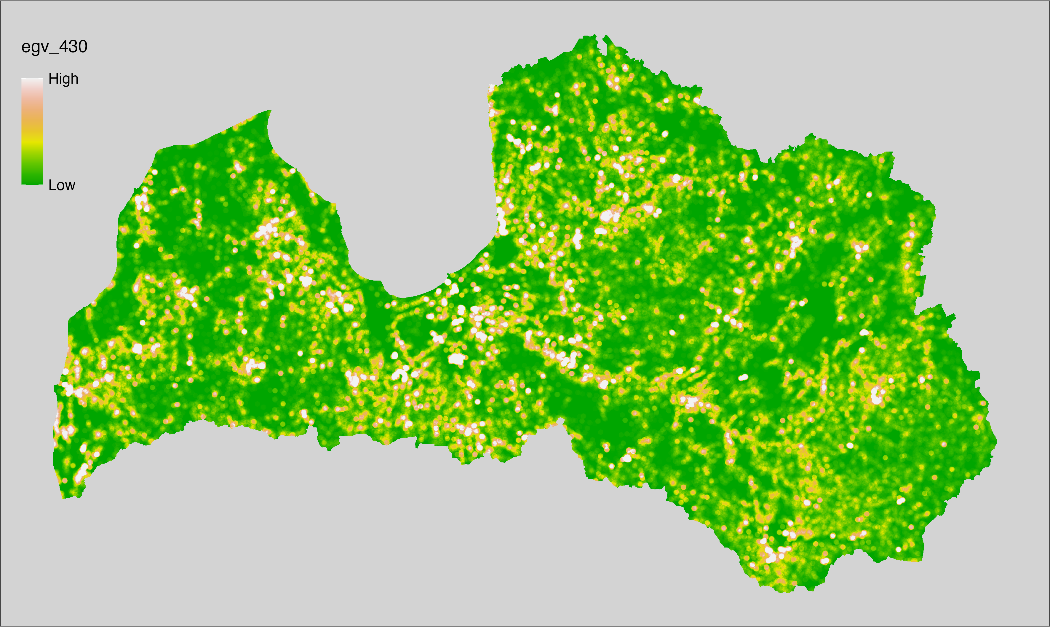
6.431 General_GardensOrchards_r3000
filename: General_GardensOrchards_r3000.tif
layername: egv_431
English name: Fractional cover of Allotment gardens, Orchards within the 3 km landscape
Latvian name: Vasarnīcu kompleksu un augļudārzu platības īpatsvars 3 km ainavā
Procedure: The cover fraction within a radius of 3000 m around the analysis grid cell
is calculated as the area-weighted sum of the analysis cells inside
the buffer, using the workflow egvtools::radius_function(). During the calculation of the landscape
metric, inverse distance weighted (power = 2) gap filling on the output is
applied to ensure no missing values at the edges. Then the layer is
rewritten to set its name. Finally, the layer is standardised by
subtracting the arithmetic mean and dividing by the root mean squared error.
Code
# libs ----
if(!require(terra)) {install.packages("terra"); require(terra)}
if(!require(egvtools)) {remotes::install_github("aavotins/egvtools"); require(egvtools)}
# Templates -----
template100=rast("./Templates/TemplateRasters/LV100m_10km.tif")
# radii ----
radius_function(
kvadrati_path = "./Templates/TemplateGrids/tiles/",
radii_path = "./Templates/TemplateGridPoints/tiles/",
tikls100_path = "./Templates/TemplateGrids/tikls100_sauzeme.parquet",
template_path = "./Templates/TemplateRasters/LV100m_10km.tif",
input_layers = c("./RasterGrids_100m/2024/RAW/General_GardensOrchards_cell.tif"),
layer_prefixes = c("General_GardensOrchards"),
output_dir = "./RasterGrids_100m/2024/RAW/",
n_workers = 6,
radii = c("r3000"),
radius_mode = "sparse",
extract_fun = "mean",
fill_missing = TRUE,
IDW_weight = 2,
future_max_size = 40 * 1024^3)
# General_GardensOrchards_r3000.tif egv_431
slanis=rast("./RasterGrids_100m/2024/RAW/General_GardensOrchards_r3000.tif")
names(slanis)="egv_431"
slanis2=project(slanis,template100)
writeRaster(slanis2,
"./RasterGrids_100m/2024/RAW/General_GardensOrchards_r3000.tif",
overwrite=TRUE)
# standardisation ----
if(!require(terra)) {install.packages("terra"); require(terra)}
if(!require(tidyverse)) {install.packages("tidyverse"); require(tidyverse)}
nosaukums="General_GardensOrchards_r3000.tif"
ielasisanas_cels=paste0("./RasterGrids_100m/2024/RAW/",nosaukums)
saglabasanas_cels=paste0("./RasterGrids_100m/2024/Scaled/",nosaukums)
slanis=rast(ielasisanas_cels)
videjais=global(slanis,fun="mean",na.rm=TRUE)
centrets=slanis-videjais[,1]
standartnovirze=terra::global(centrets,fun="rms",na.rm=TRUE)
merogots=centrets/standartnovirze[,1]
writeRaster(merogots,
filename=saglabasanas_cels,
overwrite=TRUE)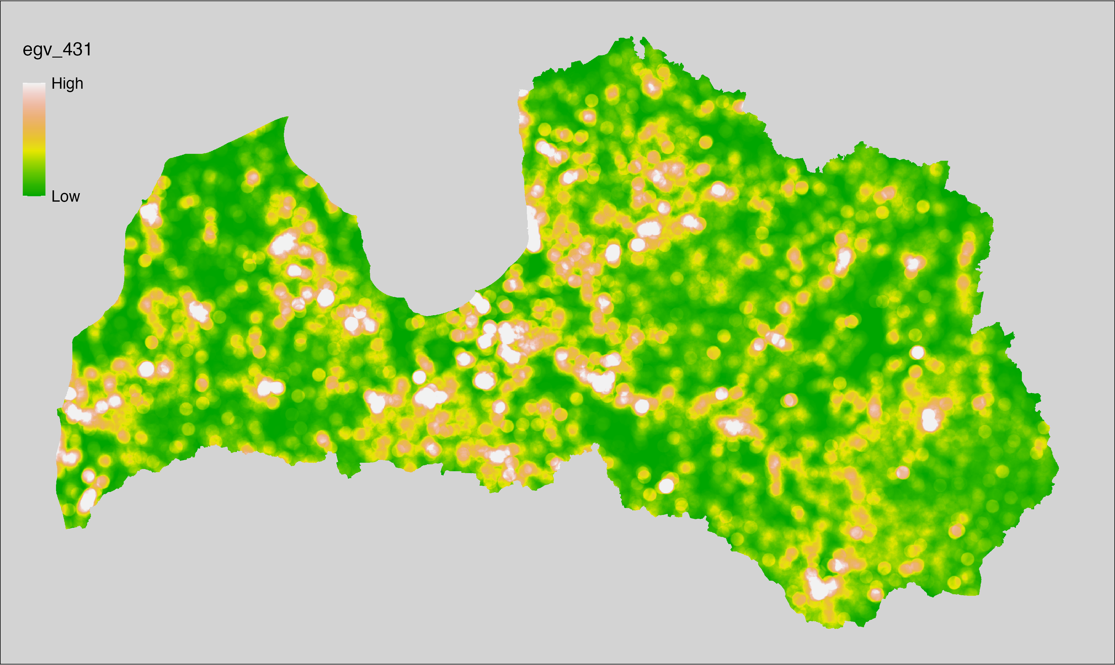
6.432 General_GardensOrchards_r10000
filename: General_GardensOrchards_r10000.tif
layername: egv_432
English name: Fractional cover of Allotment gardens, Orchards within the 10 km landscape
Latvian name: Vasarnīcu kompleksu un augļudārzu platības īpatsvars 10 km ainavā
Procedure: The cover fraction within a radius of 10000 m around the analysis grid cell
is calculated as the area-weighted sum of the analysis cells inside
the buffer, using the workflow egvtools::radius_function(). During the calculation of the landscape
metric, inverse distance weighted (power = 2) gap filling on the output is
applied to ensure no missing values at the edges. Then the layer is
rewritten to set its name. Finally, the layer is standardised by
subtracting the arithmetic mean and dividing by the root mean squared error.
Code
# libs ----
if(!require(terra)) {install.packages("terra"); require(terra)}
if(!require(egvtools)) {remotes::install_github("aavotins/egvtools"); require(egvtools)}
# Templates -----
template100=rast("./Templates/TemplateRasters/LV100m_10km.tif")
# radii ----
radius_function(
kvadrati_path = "./Templates/TemplateGrids/tiles/",
radii_path = "./Templates/TemplateGridPoints/tiles/",
tikls100_path = "./Templates/TemplateGrids/tikls100_sauzeme.parquet",
template_path = "./Templates/TemplateRasters/LV100m_10km.tif",
input_layers = c("./RasterGrids_100m/2024/RAW/General_GardensOrchards_cell.tif"),
layer_prefixes = c("General_GardensOrchards"),
output_dir = "./RasterGrids_100m/2024/RAW/",
n_workers = 6,
radii = c("r10000"),
radius_mode = "sparse",
extract_fun = "mean",
fill_missing = TRUE,
IDW_weight = 2,
future_max_size = 40 * 1024^3)
# General_GardensOrchards_r10000.tif egv_432
slanis=rast("./RasterGrids_100m/2024/RAW/General_GardensOrchards_r10000.tif")
names(slanis)="egv_432"
slanis2=project(slanis,template100)
writeRaster(slanis2,
"./RasterGrids_100m/2024/RAW/General_GardensOrchards_r10000.tif",
overwrite=TRUE)
# standardisation ----
if(!require(terra)) {install.packages("terra"); require(terra)}
if(!require(tidyverse)) {install.packages("tidyverse"); require(tidyverse)}
nosaukums="General_GardensOrchards_r10000.tif"
ielasisanas_cels=paste0("./RasterGrids_100m/2024/RAW/",nosaukums)
saglabasanas_cels=paste0("./RasterGrids_100m/2024/Scaled/",nosaukums)
slanis=rast(ielasisanas_cels)
videjais=global(slanis,fun="mean",na.rm=TRUE)
centrets=slanis-videjais[,1]
standartnovirze=terra::global(centrets,fun="rms",na.rm=TRUE)
merogots=centrets/standartnovirze[,1]
writeRaster(merogots,
filename=saglabasanas_cels,
overwrite=TRUE)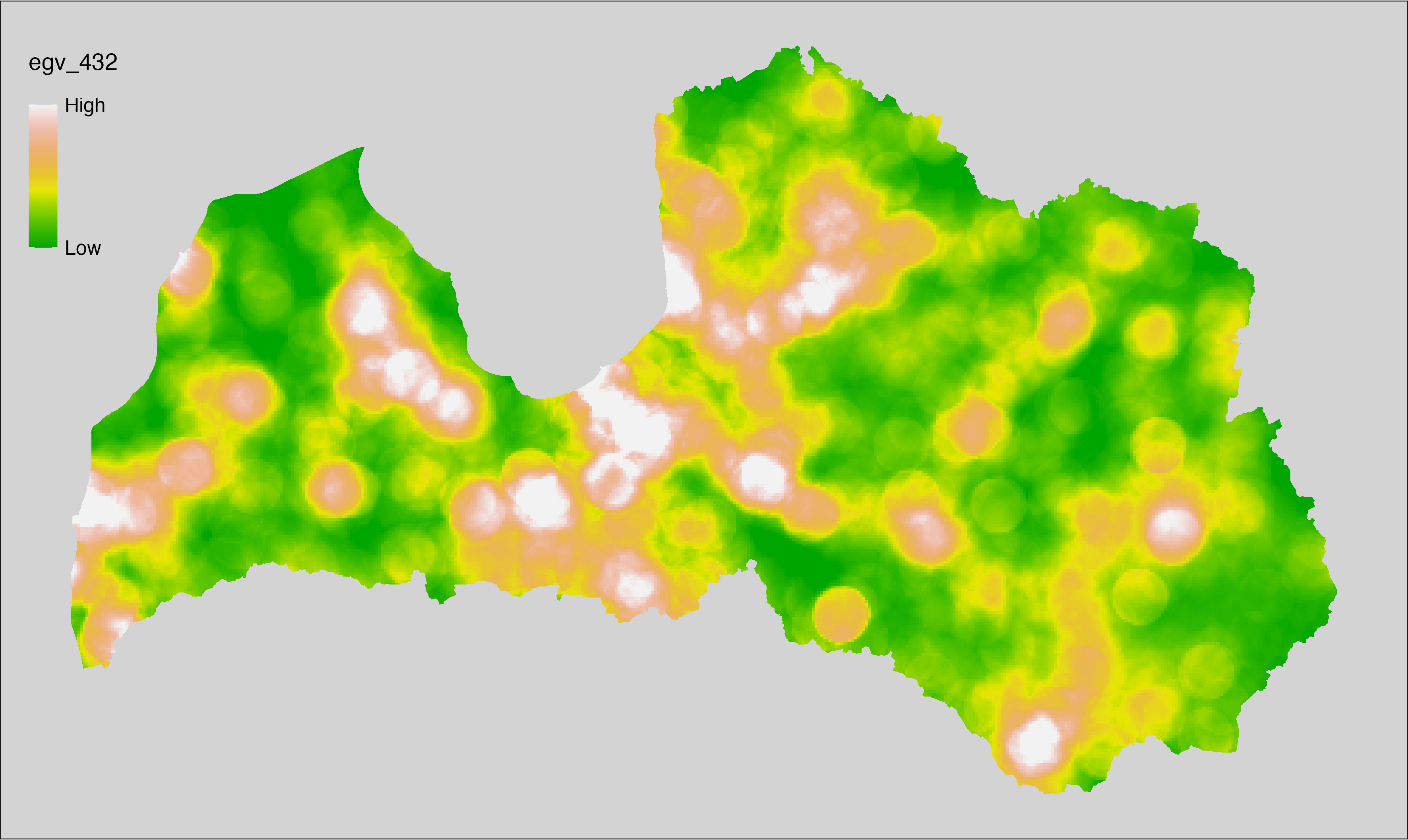
6.433 General_Roads_cell
filename: General_Roads_cell.tif
layername: egv_433
English name: Fractional cover of Roads within the analysis cell (1 ha)
Latvian name: Ceļu platības īpatsvars analīzes šūnā (1 ha)
Procedure: First, the roads from the Landscape classification are
selected (value 100 is reclassified to value 1; all others are set to 0). The resulting layer
is then aggregated to EGV resolution using the workflow egvtools::input2egv(), which
calculates the arithmetic mean to determine the cover fraction. During
aggregation, inverse distance weighted (power = 2) gap filling on the output is
applied to ensure no missing values at the edges. Finally, the layer is
standardised by subtracting the arithmetic mean and dividing by the root mean squared
error.
Code
# libs ----
if(!require(egvtools)) {remotes::install_github("aavotins/egvtools"); require(egvtools)}
if(!require(terra)) {install.packages("terra"); require(terra)}
if(!require(sf)) {install.packages("sf"); require(sf)}
if(!require(tidyverse)) {install.packages("tidyverse"); require(tidyverse)}
if(!require(sfarrow)) {install.packages("sfarrow"); require(sfarrow)}
if(!require(readxl)) {install.packages("readxl"); require(readxl)}
if(!require(raster)) {install.packages("raster"); require(raster)}
if(!require(fasterize)) {install.packages("fasterize"); require(fasterize)}
# templates ----
template100=rast("./Templates/TemplateRasters/LV100m_10km.tif")
template10=rast("./Templates/TemplateRasters/LV10m_10km.tif")
rastrs10=raster(template10)
nulls10=rast("./Templates/TemplateRasters/nulls_LV10m_10km.tif")
nulls100=rast("./Templates/TemplateRasters/nulls_LV100m_10km.tif")
# simple landscape ----
simple_landscape=rast("RasterGrids_10m/2024/Ainava_vienk_mask.tif")
# General_Roads_cell.tif egv_433 ----
celi=ifel(simple_landscape==100,1,0)
i2e_rez=egvtools::input2egv(input=celi,
egv_template= "./Templates/TemplateRasters/LV100m_10km.tif",
summary_function = "average",
missing_job = "FillOutput",
outlocation = "./RasterGrids_100m/2024/RAW/",
outfilename = "General_Roads_cell.tif",
layername = "egv_433",
idw_weight = 2,
plot_gaps = FALSE,plot_final = TRUE)
i2e_rez
rm(celi)
rm(i2e_rez)
# standardisation ----
if(!require(terra)) {install.packages("terra"); require(terra)}
if(!require(tidyverse)) {install.packages("tidyverse"); require(tidyverse)}
nosaukums="General_Roads_cell.tif"
ielasisanas_cels=paste0("./RasterGrids_100m/2024/RAW/",nosaukums)
saglabasanas_cels=paste0("./RasterGrids_100m/2024/Scaled/",nosaukums)
slanis=rast(ielasisanas_cels)
videjais=global(slanis,fun="mean",na.rm=TRUE)
centrets=slanis-videjais[,1]
standartnovirze=terra::global(centrets,fun="rms",na.rm=TRUE)
merogots=centrets/standartnovirze[,1]
writeRaster(merogots,
filename=saglabasanas_cels,
overwrite=TRUE)
6.434 General_ShrubsOrchards_cell
filename: General_ShrubsOrchards_cell.tif
layername: egv_434
English name: Fractional cover of Shrubs, Young stands, Orchards within the analysis cell (1 ha)
Latvian name: Krūmāju, jaunaudžu un augļudārzu platības īpatsvars analīzes šūnā (1 ha)
Procedure: First, agricultural parcels declared as short term coppice are
selected from the Rural Support Service’s information on declared fields
and rasterised to match inputs. Then orchards and shrubs-low forest stands from
Landscape classification are selected (values equal to 420 or 620
are reclassified to value 1, others as 0). The first layer is then covered
over the second. The resulting layer
is then aggregated to EGV resolution using the workflow egvtools::input2egv(), which
calculates the arithmetic mean to determine the cover fraction. During
aggregation, inverse distance weighted (power = 2) gap filling on the output is
applied to ensure no missing values at the edges. Finally, the layer is
standardised by subtracting the arithmetic mean and dividing by the root mean squared
error.
Code
# libs ----
if(!require(egvtools)) {remotes::install_github("aavotins/egvtools"); require(egvtools)}
if(!require(terra)) {install.packages("terra"); require(terra)}
if(!require(sf)) {install.packages("sf"); require(sf)}
if(!require(tidyverse)) {install.packages("tidyverse"); require(tidyverse)}
if(!require(sfarrow)) {install.packages("sfarrow"); require(sfarrow)}
if(!require(readxl)) {install.packages("readxl"); require(readxl)}
if(!require(raster)) {install.packages("raster"); require(raster)}
if(!require(fasterize)) {install.packages("fasterize"); require(fasterize)}
# templates ----
template100=rast("./Templates/TemplateRasters/LV100m_10km.tif")
template10=rast("./Templates/TemplateRasters/LV10m_10km.tif")
rastrs10=raster(template10)
nulls10=rast("./Templates/TemplateRasters/nulls_LV10m_10km.tif")
nulls100=rast("./Templates/TemplateRasters/nulls_LV100m_10km.tif")
# simple landscape ----
simple_landscape=rast("RasterGrids_10m/2024/Ainava_vienk_mask.tif")
# General_ShrubsOrchards_cell.tif egv_434 ----
kodi=read_excel("./Geodata/2024/LAD/KulturuKodi_2024.xlsx")
kodi$kods=as.character(kodi$kods)
table(kodi$SDM_grupa_sakums,useNA="always")
lad=sfarrow::st_read_parquet("./Geodata/2024/LAD/Lauki_2024.parquet")
lad$yes=1
lad=lad %>%
left_join(kodi,by=c("PRODUCT_CODE"="kods"))
ilggadigiekrumveida=lad %>%
filter(SDM_grupa_sakums == "krūmveida ilggadīgie stādījumi")
krumveida_r=fasterize(ilggadigiekrumveida,rastrs10,field="yes",fun="first")
krumveida_t=rast(krumveida_r)
augludarzi=ifel(simple_landscape==420|simple_landscape==620,1,0)
apvienoti=cover(krumveida_t,augludarzi)
plot(apvienoti)
i2e_rez=egvtools::input2egv(input=apvienoti,
egv_template= "./Templates/TemplateRasters/LV100m_10km.tif",
summary_function = "average",
missing_job = "FillOutput",
outlocation = "./RasterGrids_100m/2024/RAW/",
outfilename = "General_ShrubsOrchards_cell.tif",
layername = "egv_434",
idw_weight = 2,
plot_gaps = FALSE,plot_final = TRUE)
i2e_rez
rm(apvienoti)
rm(i2e_rez)
rm(ilggadigiekrumveida)
rm(krumveida_r)
rm(krumveida_t)
rm(augludarzi)
rm(kodi)
rm(lad)
# standardisation ----
if(!require(terra)) {install.packages("terra"); require(terra)}
if(!require(tidyverse)) {install.packages("tidyverse"); require(tidyverse)}
nosaukums="General_ShrubsOrchards_cell.tif"
ielasisanas_cels=paste0("./RasterGrids_100m/2024/RAW/",nosaukums)
saglabasanas_cels=paste0("./RasterGrids_100m/2024/Scaled/",nosaukums)
slanis=rast(ielasisanas_cels)
videjais=global(slanis,fun="mean",na.rm=TRUE)
centrets=slanis-videjais[,1]
standartnovirze=terra::global(centrets,fun="rms",na.rm=TRUE)
merogots=centrets/standartnovirze[,1]
writeRaster(merogots,
filename=saglabasanas_cels,
overwrite=TRUE)
6.435 General_ShrubsOrchards_r500
filename: General_ShrubsOrchards_r500.tif
layername: egv_435
English name: Fractional cover of Shrubs, Young stands, Orchards within the 0.5 km landscape
Latvian name: Krūmāju, jaunaudžu un augļudārzu platības īpatsvars 0,5 km ainavā
Procedure: The cover fraction within a radius of 500 m around the analysis grid cell is
calculated as the area-weighted sum of the analysis cells inside the
buffer, using the workflow egvtools::radius_function(). During the calculation of the landscape metric,
inverse distance weighted (power = 2) gap filling on the output is applied
to ensure no missing values at the edges. Then the layer is rewritten to set
its name. Finally, the layer is standardised by subtracting the arithmetic
mean and dividing by the root mean squared error.
Code
# libs ----
if(!require(terra)) {install.packages("terra"); require(terra)}
if(!require(egvtools)) {remotes::install_github("aavotins/egvtools"); require(egvtools)}
# Templates -----
template100=rast("./Templates/TemplateRasters/LV100m_10km.tif")
# radii ----
radius_function(
kvadrati_path = "./Templates/TemplateGrids/tiles/",
radii_path = "./Templates/TemplateGridPoints/tiles/",
tikls100_path = "./Templates/TemplateGrids/tikls100_sauzeme.parquet",
template_path = "./Templates/TemplateRasters/LV100m_10km.tif",
input_layers = c("./RasterGrids_100m/2024/RAW/General_ShrubsOrchards_cell.tif"),
layer_prefixes = c("General_ShrubsOrchards"),
output_dir = "./RasterGrids_100m/2024/RAW/",
n_workers = 6,
radii = c("r500"),
radius_mode = "sparse",
extract_fun = "mean",
fill_missing = TRUE,
IDW_weight = 2,
future_max_size = 40 * 1024^3)
# General_ShrubsOrchards_r500.tif egv_435
slanis=rast("./RasterGrids_100m/2024/RAW/General_ShrubsOrchards_r500.tif")
names(slanis)="egv_435"
slanis2=project(slanis,template100)
writeRaster(slanis2,
"./RasterGrids_100m/2024/RAW/General_ShrubsOrchards_r500.tif",
overwrite=TRUE)
# standardisation ----
if(!require(terra)) {install.packages("terra"); require(terra)}
if(!require(tidyverse)) {install.packages("tidyverse"); require(tidyverse)}
nosaukums="General_ShrubsOrchards_r500.tif"
ielasisanas_cels=paste0("./RasterGrids_100m/2024/RAW/",nosaukums)
saglabasanas_cels=paste0("./RasterGrids_100m/2024/Scaled/",nosaukums)
slanis=rast(ielasisanas_cels)
videjais=global(slanis,fun="mean",na.rm=TRUE)
centrets=slanis-videjais[,1]
standartnovirze=terra::global(centrets,fun="rms",na.rm=TRUE)
merogots=centrets/standartnovirze[,1]
writeRaster(merogots,
filename=saglabasanas_cels,
overwrite=TRUE)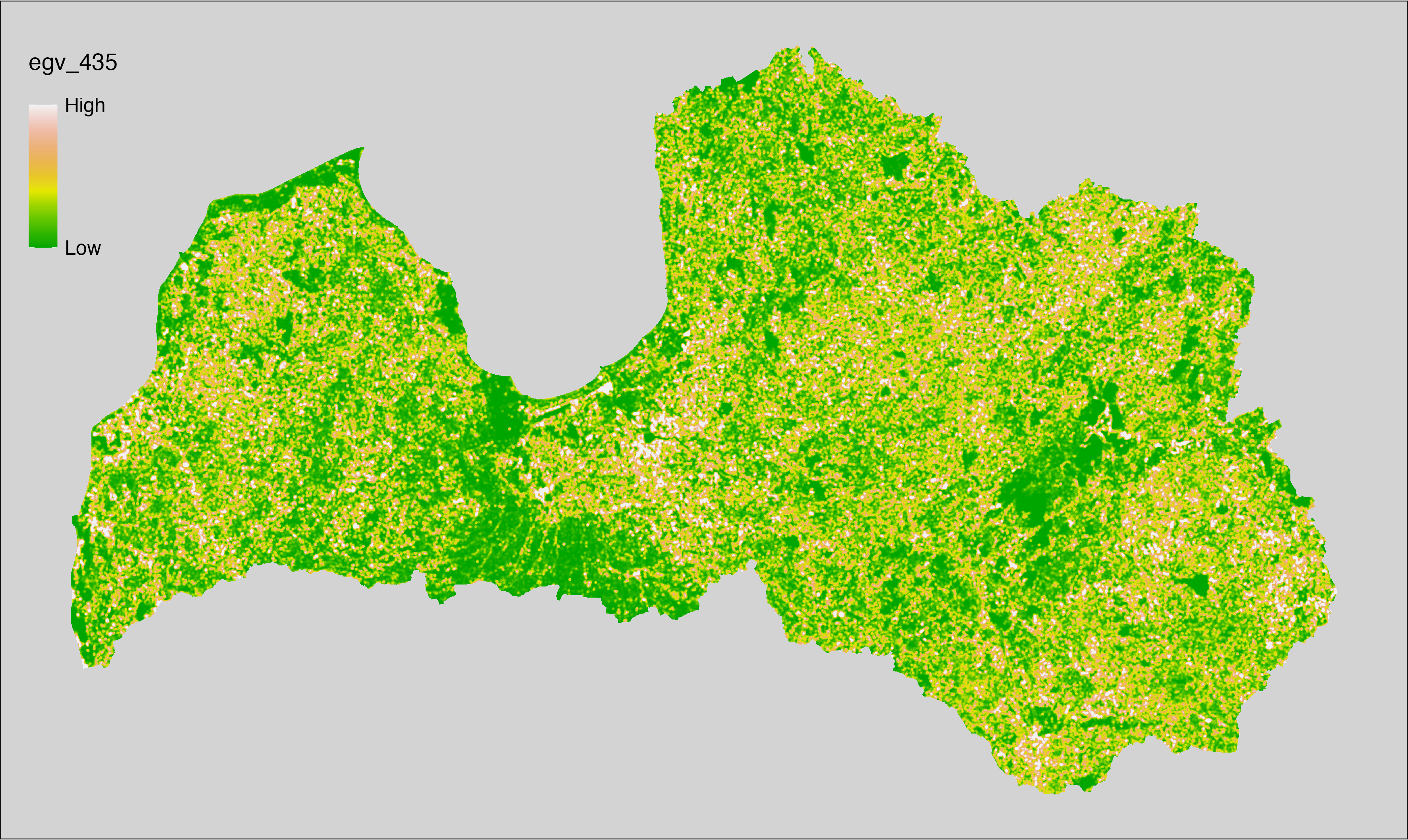
6.436 General_ShrubsOrchards_r1250
filename: General_ShrubsOrchards_r1250.tif
layername: egv_436
English name: Fractional cover of Shrubs, Young stands, Orchards within the 1.25 km landscape
Latvian name: Krūmāju, jaunaudžu un augļudārzu platības īpatsvars 1,25 km ainavā
Procedure: The cover fraction within a radius of 1250 m around the analysis grid cell
is calculated as the area-weighted sum of the analysis cells inside
the buffer, using the workflow egvtools::radius_function(). During the calculation of the landscape
metric, inverse distance weighted (power = 2) gap filling on the output is
applied to ensure no missing values at the edges. Then the layer is
rewritten to set its name. Finally, the layer is standardised by
subtracting the arithmetic mean and dividing by the root mean squared error.
Code
# libs ----
if(!require(terra)) {install.packages("terra"); require(terra)}
if(!require(egvtools)) {remotes::install_github("aavotins/egvtools"); require(egvtools)}
# Templates -----
template100=rast("./Templates/TemplateRasters/LV100m_10km.tif")
# radii ----
radius_function(
kvadrati_path = "./Templates/TemplateGrids/tiles/",
radii_path = "./Templates/TemplateGridPoints/tiles/",
tikls100_path = "./Templates/TemplateGrids/tikls100_sauzeme.parquet",
template_path = "./Templates/TemplateRasters/LV100m_10km.tif",
input_layers = c("./RasterGrids_100m/2024/RAW/General_ShrubsOrchards_cell.tif"),
layer_prefixes = c("General_ShrubsOrchards"),
output_dir = "./RasterGrids_100m/2024/RAW/",
n_workers = 6,
radii = c("r1250"),
radius_mode = "sparse",
extract_fun = "mean",
fill_missing = TRUE,
IDW_weight = 2,
future_max_size = 40 * 1024^3)
# General_ShrubsOrchards_r1250.tif egv_436
slanis=rast("./RasterGrids_100m/2024/RAW/General_ShrubsOrchards_r1250.tif")
names(slanis)="egv_436"
slanis2=project(slanis,template100)
writeRaster(slanis2,
"./RasterGrids_100m/2024/RAW/General_ShrubsOrchards_r1250.tif",
overwrite=TRUE)
# standardisation ----
if(!require(terra)) {install.packages("terra"); require(terra)}
if(!require(tidyverse)) {install.packages("tidyverse"); require(tidyverse)}
nosaukums="General_ShrubsOrchards_r1250.tif"
ielasisanas_cels=paste0("./RasterGrids_100m/2024/RAW/",nosaukums)
saglabasanas_cels=paste0("./RasterGrids_100m/2024/Scaled/",nosaukums)
slanis=rast(ielasisanas_cels)
videjais=global(slanis,fun="mean",na.rm=TRUE)
centrets=slanis-videjais[,1]
standartnovirze=terra::global(centrets,fun="rms",na.rm=TRUE)
merogots=centrets/standartnovirze[,1]
writeRaster(merogots,
filename=saglabasanas_cels,
overwrite=TRUE)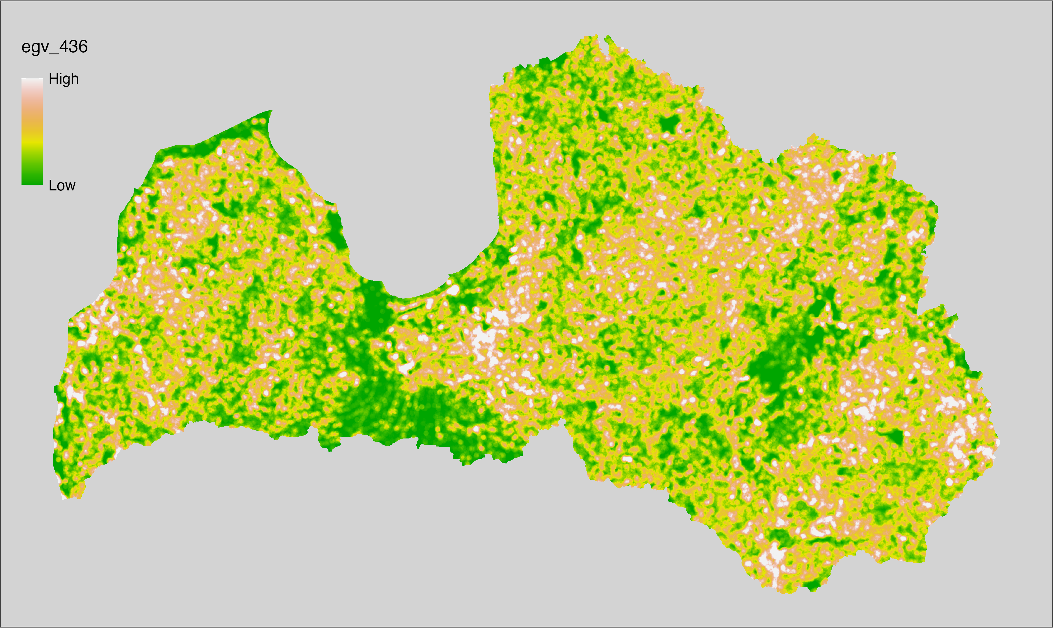
6.437 General_ShrubsOrchards_r3000
filename: General_ShrubsOrchards_r3000.tif
layername: egv_437
English name: Fractional cover of Shrubs, Young stands, Orchards within the 3 km landscape
Latvian name: Krūmāju, jaunaudžu un augļudārzu platības īpatsvars 3 km ainavā
Procedure: The cover fraction within a radius of 3000 m around the analysis grid cell
is calculated as the area-weighted sum of the analysis cells inside
the buffer, using the workflow egvtools::radius_function(). During the calculation of the landscape
metric, inverse distance weighted (power = 2) gap filling on the output is
applied to ensure no missing values at the edges. Then the layer is
rewritten to set its name. Finally, the layer is standardised by
subtracting the arithmetic mean and dividing by the root mean squared error.
Code
# libs ----
if(!require(terra)) {install.packages("terra"); require(terra)}
if(!require(egvtools)) {remotes::install_github("aavotins/egvtools"); require(egvtools)}
# Templates -----
template100=rast("./Templates/TemplateRasters/LV100m_10km.tif")
# radii ----
radius_function(
kvadrati_path = "./Templates/TemplateGrids/tiles/",
radii_path = "./Templates/TemplateGridPoints/tiles/",
tikls100_path = "./Templates/TemplateGrids/tikls100_sauzeme.parquet",
template_path = "./Templates/TemplateRasters/LV100m_10km.tif",
input_layers = c("./RasterGrids_100m/2024/RAW/General_ShrubsOrchards_cell.tif"),
layer_prefixes = c("General_ShrubsOrchards"),
output_dir = "./RasterGrids_100m/2024/RAW/",
n_workers = 6,
radii = c("r3000"),
radius_mode = "sparse",
extract_fun = "mean",
fill_missing = TRUE,
IDW_weight = 2,
future_max_size = 40 * 1024^3)
# General_ShrubsOrchards_r3000.tif egv_437
slanis=rast("./RasterGrids_100m/2024/RAW/General_ShrubsOrchards_r3000.tif")
names(slanis)="egv_437"
slanis2=project(slanis,template100)
writeRaster(slanis2,
"./RasterGrids_100m/2024/RAW/General_ShrubsOrchards_r3000.tif",
overwrite=TRUE)
# standardisation ----
if(!require(terra)) {install.packages("terra"); require(terra)}
if(!require(tidyverse)) {install.packages("tidyverse"); require(tidyverse)}
nosaukums="General_ShrubsOrchards_r3000.tif"
ielasisanas_cels=paste0("./RasterGrids_100m/2024/RAW/",nosaukums)
saglabasanas_cels=paste0("./RasterGrids_100m/2024/Scaled/",nosaukums)
slanis=rast(ielasisanas_cels)
videjais=global(slanis,fun="mean",na.rm=TRUE)
centrets=slanis-videjais[,1]
standartnovirze=terra::global(centrets,fun="rms",na.rm=TRUE)
merogots=centrets/standartnovirze[,1]
writeRaster(merogots,
filename=saglabasanas_cels,
overwrite=TRUE)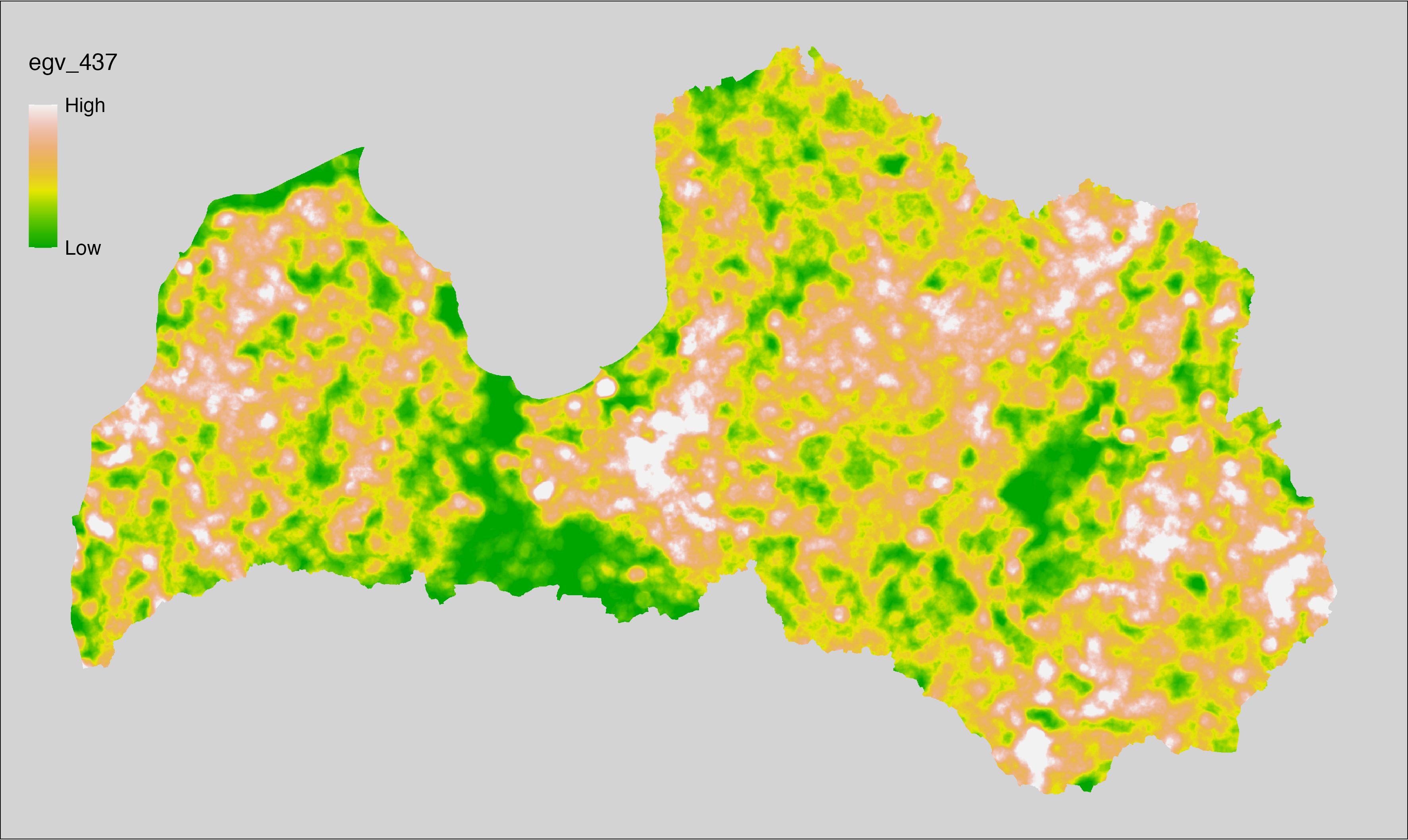
6.438 General_ShrubsOrchards_r10000
filename: General_ShrubsOrchards_r10000.tif
layername: egv_438
English name: Fractional cover of Shrubs, Young stands, Orchards within the 10 km landscape
Latvian name: Krūmāju, jaunaudžu un augļudārzu platības īpatsvars 10 km ainavā
Procedure: The cover fraction within a radius of 10000 m around the analysis grid cell
is calculated as the area-weighted sum of the analysis cells inside
the buffer, using the workflow egvtools::radius_function(). During the calculation of the landscape
metric, inverse distance weighted (power = 2) gap filling on the output is
applied to ensure no missing values at the edges. Then the layer is
rewritten to set its name. Finally, the layer is standardised by
subtracting the arithmetic mean and dividing by the root mean squared error.
Code
# libs ----
if(!require(terra)) {install.packages("terra"); require(terra)}
if(!require(egvtools)) {remotes::install_github("aavotins/egvtools"); require(egvtools)}
# Templates -----
template100=rast("./Templates/TemplateRasters/LV100m_10km.tif")
# radii ----
radius_function(
kvadrati_path = "./Templates/TemplateGrids/tiles/",
radii_path = "./Templates/TemplateGridPoints/tiles/",
tikls100_path = "./Templates/TemplateGrids/tikls100_sauzeme.parquet",
template_path = "./Templates/TemplateRasters/LV100m_10km.tif",
input_layers = c("./RasterGrids_100m/2024/RAW/General_ShrubsOrchards_cell.tif"),
layer_prefixes = c("General_ShrubsOrchards"),
output_dir = "./RasterGrids_100m/2024/RAW/",
n_workers = 6,
radii = c("r10000"),
radius_mode = "sparse",
extract_fun = "mean",
fill_missing = TRUE,
IDW_weight = 2,
future_max_size = 40 * 1024^3)
# General_ShrubsOrchards_r10000.tif egv_438
slanis=rast("./RasterGrids_100m/2024/RAW/General_ShrubsOrchards_r10000.tif")
names(slanis)="egv_438"
slanis2=project(slanis,template100)
writeRaster(slanis2,
"./RasterGrids_100m/2024/RAW/General_ShrubsOrchards_r10000.tif",
overwrite=TRUE)
# standardisation ----
if(!require(terra)) {install.packages("terra"); require(terra)}
if(!require(tidyverse)) {install.packages("tidyverse"); require(tidyverse)}
nosaukums="General_ShrubsOrchards_r10000.tif"
ielasisanas_cels=paste0("./RasterGrids_100m/2024/RAW/",nosaukums)
saglabasanas_cels=paste0("./RasterGrids_100m/2024/Scaled/",nosaukums)
slanis=rast(ielasisanas_cels)
videjais=global(slanis,fun="mean",na.rm=TRUE)
centrets=slanis-videjais[,1]
standartnovirze=terra::global(centrets,fun="rms",na.rm=TRUE)
merogots=centrets/standartnovirze[,1]
writeRaster(merogots,
filename=saglabasanas_cels,
overwrite=TRUE)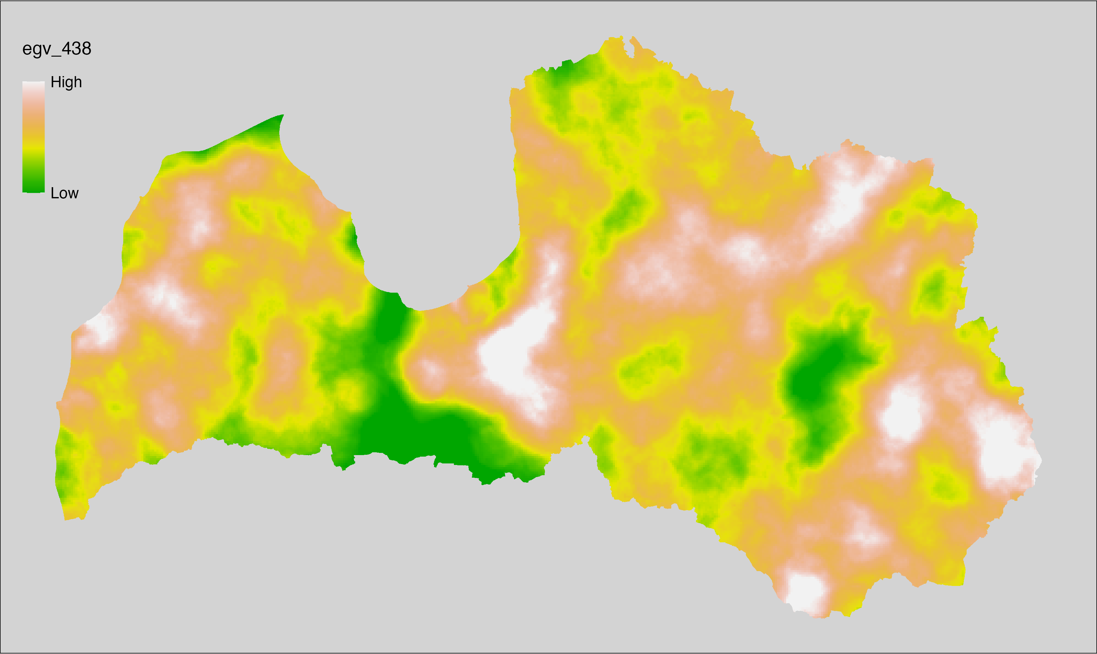
6.439 General_ShrubsOrchardsGardens_cell
filename: General_ShrubsOrchardsGardens_cell.tif
layername: egv_439
English name: Fractional cover of Shrubs, Young stands, Orchards, Allotment gardens within the analysis cell (1 ha)
Latvian name: Krūmāju, jaunaudžu, augļudārzu un vasarnīcu kompleksu platības īpatsvars analīzes šūnā (1 ha)
Procedure: First, agricultural parcels declared as short term coppice are
selected from the Rural Support Service’s information on declared fields
and rasterised to match inputs. Then orchards, allotment gardens and shrubs-low
forest stands from the Landscape classification are selected (values
between 400 and 500 or equal to 620 are reclassified to value 1, others as 0).
The first layer is then covered over the second. The resulting layer
is then aggregated to EGV resolution using the workflow egvtools::input2egv(), which
calculates the arithmetic mean to determine the cover fraction. During
aggregation, inverse distance weighted (power = 2) gap filling on the output is
applied to ensure no missing values at the edges. Finally, the layer is
standardised by subtracting the arithmetic mean and dividing by the root mean squared
error.
Code
# libs ----
if(!require(egvtools)) {remotes::install_github("aavotins/egvtools"); require(egvtools)}
if(!require(terra)) {install.packages("terra"); require(terra)}
if(!require(sf)) {install.packages("sf"); require(sf)}
if(!require(tidyverse)) {install.packages("tidyverse"); require(tidyverse)}
if(!require(sfarrow)) {install.packages("sfarrow"); require(sfarrow)}
if(!require(readxl)) {install.packages("readxl"); require(readxl)}
if(!require(raster)) {install.packages("raster"); require(raster)}
if(!require(fasterize)) {install.packages("fasterize"); require(fasterize)}
# templates ----
template100=rast("./Templates/TemplateRasters/LV100m_10km.tif")
template10=rast("./Templates/TemplateRasters/LV10m_10km.tif")
rastrs10=raster(template10)
nulls10=rast("./Templates/TemplateRasters/nulls_LV10m_10km.tif")
nulls100=rast("./Templates/TemplateRasters/nulls_LV100m_10km.tif")
# simple landscape ----
simple_landscape=rast("RasterGrids_10m/2024/Ainava_vienk_mask.tif")
# General_ShrubsOrchardsGardens_cell.tif egv_439 ----
kodi=read_excel("./Geodata/2024/LAD/KulturuKodi_2024.xlsx")
kodi$kods=as.character(kodi$kods)
table(kodi$SDM_grupa_sakums,useNA="always")
lad=sfarrow::st_read_parquet("./Geodata/2024/LAD/Lauki_2024.parquet")
lad$yes=1
lad=lad %>%
left_join(kodi,by=c("PRODUCT_CODE"="kods"))
ilggadigiekrumveida=lad %>%
filter(SDM_grupa_sakums == "krūmveida ilggadīgie stādījumi")
krumveida_r=fasterize(ilggadigiekrumveida,rastrs10,field="yes",fun="first")
krumveida_t=rast(krumveida_r)
parejie=ifel((simple_landscape>=400&simple_landscape<500)|
simple_landscape==620,1,0)
apvienoti=cover(krumveida_t,parejie)
plot(apvienoti)
i2e_rez=egvtools::input2egv(input=apvienoti,
egv_template= "./Templates/TemplateRasters/LV100m_10km.tif",
summary_function = "average",
missing_job = "FillOutput",
outlocation = "./RasterGrids_100m/2024/RAW/",
outfilename = "General_ShrubsOrchardsGardens_cell.tif",
layername = "egv_439",
idw_weight = 2,
plot_gaps = FALSE,plot_final = TRUE)
i2e_rez
rm(apvienoti)
rm(i2e_rez)
rm(ilggadigiekrumveida)
rm(krumveida_r)
rm(krumveida_t)
rm(parejie)
# standardisation ----
if(!require(terra)) {install.packages("terra"); require(terra)}
if(!require(tidyverse)) {install.packages("tidyverse"); require(tidyverse)}
nosaukums="General_ShrubsOrchardsGardens_cell.tif"
ielasisanas_cels=paste0("./RasterGrids_100m/2024/RAW/",nosaukums)
saglabasanas_cels=paste0("./RasterGrids_100m/2024/Scaled/",nosaukums)
slanis=rast(ielasisanas_cels)
videjais=global(slanis,fun="mean",na.rm=TRUE)
centrets=slanis-videjais[,1]
standartnovirze=terra::global(centrets,fun="rms",na.rm=TRUE)
merogots=centrets/standartnovirze[,1]
writeRaster(merogots,
filename=saglabasanas_cels,
overwrite=TRUE)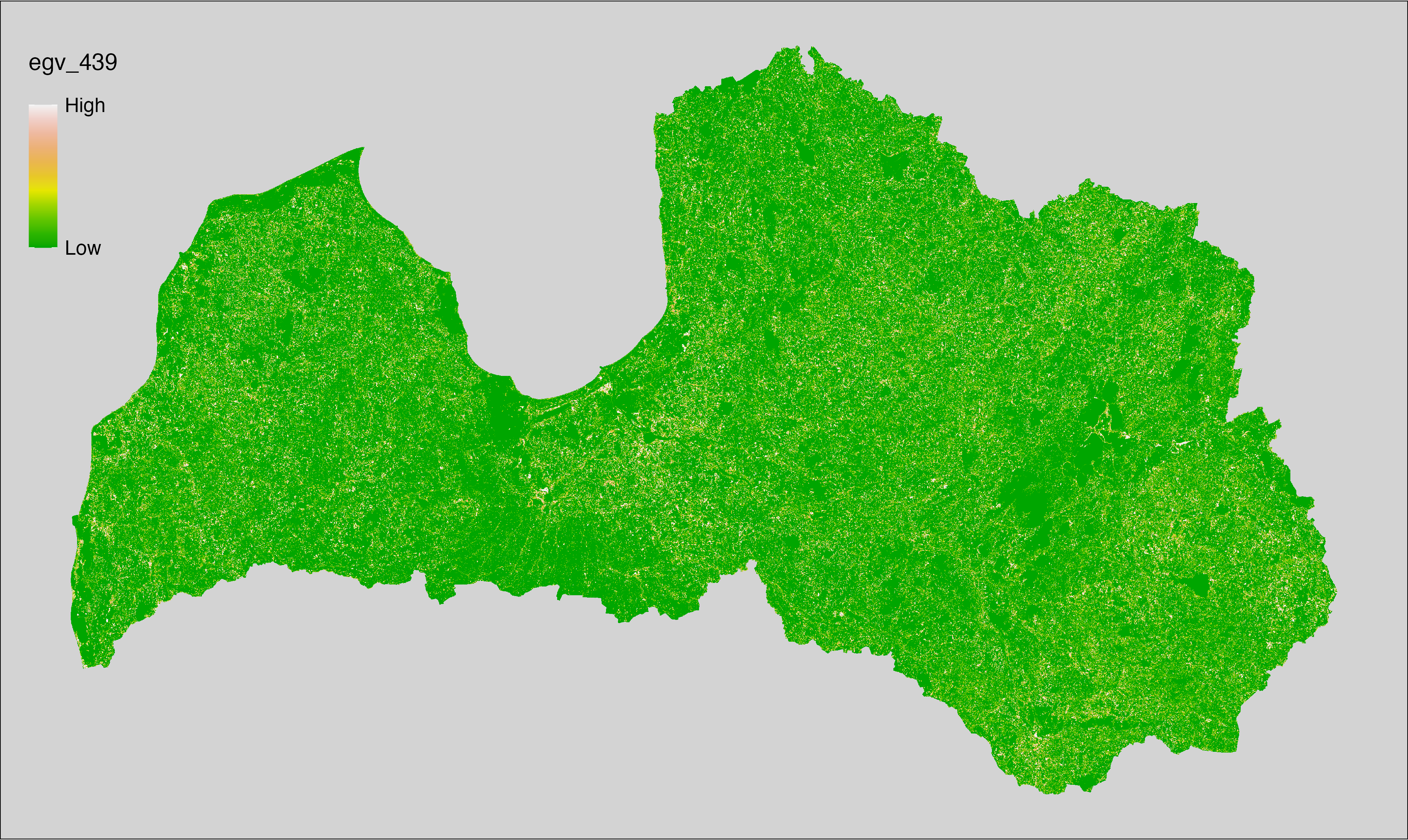
6.440 General_ShrubsOrchardsGardens_r500
filename: General_ShrubsOrchardsGardens_r500.tif
layername: egv_440
English name: Fractional cover of Shrubs, Young stands, Orchards, Allotment gardens within the 0.5 km landscape
Latvian name: Krūmāju, jaunaudžu, augļudārzu un vasarnīcu kompleksu platības īpatsvars 0,5 km ainavā
Procedure: The cover fraction within a radius of 500 m around the analysis grid cell is
calculated as the area-weighted sum of the analysis cells inside the
buffer, using the workflow egvtools::radius_function(). During the calculation of the landscape metric,
inverse distance weighted (power = 2) gap filling on the output is applied
to ensure no missing values at the edges. Then the layer is rewritten to set
its name. Finally, the layer is standardised by subtracting the arithmetic
mean and dividing by the root mean squared error.
Code
# libs ----
if(!require(terra)) {install.packages("terra"); require(terra)}
if(!require(egvtools)) {remotes::install_github("aavotins/egvtools"); require(egvtools)}
# Templates -----
template100=rast("./Templates/TemplateRasters/LV100m_10km.tif")
# radii ----
radius_function(
kvadrati_path = "./Templates/TemplateGrids/tiles/",
radii_path = "./Templates/TemplateGridPoints/tiles/",
tikls100_path = "./Templates/TemplateGrids/tikls100_sauzeme.parquet",
template_path = "./Templates/TemplateRasters/LV100m_10km.tif",
input_layers = c("./RasterGrids_100m/2024/RAW/General_ShrubsOrchardsGardens_cell.tif"),
layer_prefixes = c("General_ShrubsOrchardsGardens"),
output_dir = "./RasterGrids_100m/2024/RAW/",
n_workers = 6,
radii = c("r500"),
radius_mode = "sparse",
extract_fun = "mean",
fill_missing = TRUE,
IDW_weight = 2,
future_max_size = 40 * 1024^3)
# General_ShrubsOrchardsGardens_r500.tif egv_440
slanis=rast("./RasterGrids_100m/2024/RAW/General_ShrubsOrchardsGardens_r500.tif")
names(slanis)="egv_440"
slanis2=project(slanis,template100)
writeRaster(slanis2,
"./RasterGrids_100m/2024/RAW/General_ShrubsOrchardsGardens_r500.tif",
overwrite=TRUE)
# standardisation ----
if(!require(terra)) {install.packages("terra"); require(terra)}
if(!require(tidyverse)) {install.packages("tidyverse"); require(tidyverse)}
nosaukums="General_ShrubsOrchardsGardens_r500.tif"
ielasisanas_cels=paste0("./RasterGrids_100m/2024/RAW/",nosaukums)
saglabasanas_cels=paste0("./RasterGrids_100m/2024/Scaled/",nosaukums)
slanis=rast(ielasisanas_cels)
videjais=global(slanis,fun="mean",na.rm=TRUE)
centrets=slanis-videjais[,1]
standartnovirze=terra::global(centrets,fun="rms",na.rm=TRUE)
merogots=centrets/standartnovirze[,1]
writeRaster(merogots,
filename=saglabasanas_cels,
overwrite=TRUE)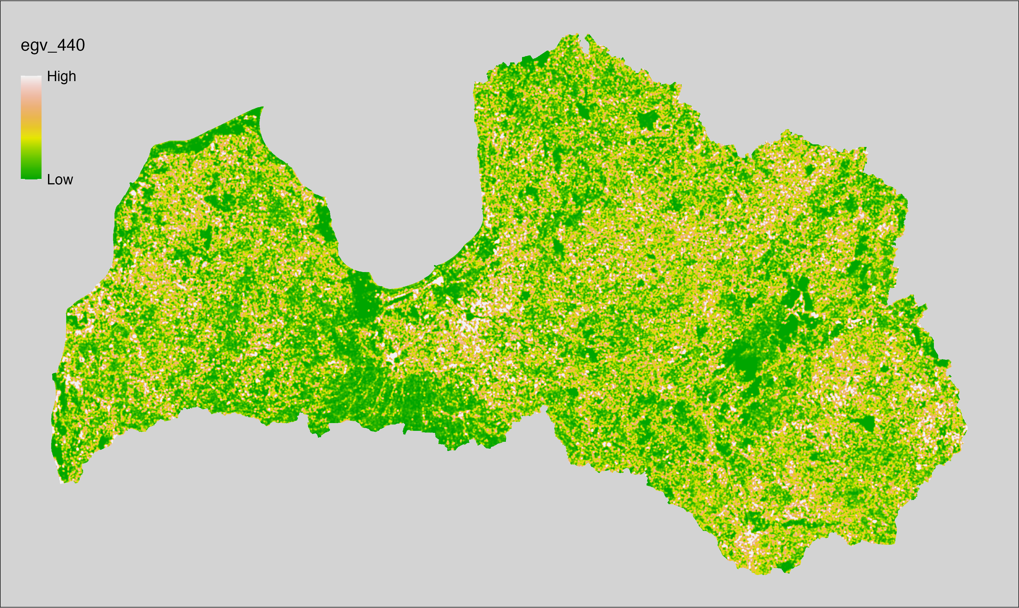
6.441 General_ShrubsOrchardsGardens_r1250
filename: General_ShrubsOrchardsGardens_r1250.tif
layername: egv_441
English name: Fractional cover of Shrubs, Young stands, Orchards, Allotment gardens within the 1.25 km landscape
Latvian name: Krūmāju, jaunaudžu, augļudārzu un vasarnīcu kompleksu platības īpatsvars 1,25 km ainavā
Procedure: The cover fraction within a radius of 1250 m around the analysis grid cell
is calculated as the area-weighted sum of the analysis cells inside
the buffer, using the workflow egvtools::radius_function(). During the calculation of the landscape
metric, inverse distance weighted (power = 2) gap filling on the output is
applied to ensure no missing values at the edges. Then the layer is
rewritten to set its name. Finally, the layer is standardised by
subtracting the arithmetic mean and dividing by the root mean squared error.
Code
# libs ----
if(!require(terra)) {install.packages("terra"); require(terra)}
if(!require(egvtools)) {remotes::install_github("aavotins/egvtools"); require(egvtools)}
# Templates -----
template100=rast("./Templates/TemplateRasters/LV100m_10km.tif")
# radii ----
radius_function(
kvadrati_path = "./Templates/TemplateGrids/tiles/",
radii_path = "./Templates/TemplateGridPoints/tiles/",
tikls100_path = "./Templates/TemplateGrids/tikls100_sauzeme.parquet",
template_path = "./Templates/TemplateRasters/LV100m_10km.tif",
input_layers = c("./RasterGrids_100m/2024/RAW/General_ShrubsOrchardsGardens_cell.tif"),
layer_prefixes = c("General_ShrubsOrchardsGardens"),
output_dir = "./RasterGrids_100m/2024/RAW/",
n_workers = 6,
radii = c("r1250"),
radius_mode = "sparse",
extract_fun = "mean",
fill_missing = TRUE,
IDW_weight = 2,
future_max_size = 40 * 1024^3)
# General_ShrubsOrchardsGardens_r1250.tif egv_441
slanis=rast("./RasterGrids_100m/2024/RAW/General_ShrubsOrchardsGardens_r1250.tif")
names(slanis)="egv_441"
slanis2=project(slanis,template100)
writeRaster(slanis2,
"./RasterGrids_100m/2024/RAW/General_ShrubsOrchardsGardens_r1250.tif",
overwrite=TRUE)
# standardisation ----
if(!require(terra)) {install.packages("terra"); require(terra)}
if(!require(tidyverse)) {install.packages("tidyverse"); require(tidyverse)}
nosaukums="General_ShrubsOrchardsGardens_r1250.tif"
ielasisanas_cels=paste0("./RasterGrids_100m/2024/RAW/",nosaukums)
saglabasanas_cels=paste0("./RasterGrids_100m/2024/Scaled/",nosaukums)
slanis=rast(ielasisanas_cels)
videjais=global(slanis,fun="mean",na.rm=TRUE)
centrets=slanis-videjais[,1]
standartnovirze=terra::global(centrets,fun="rms",na.rm=TRUE)
merogots=centrets/standartnovirze[,1]
writeRaster(merogots,
filename=saglabasanas_cels,
overwrite=TRUE)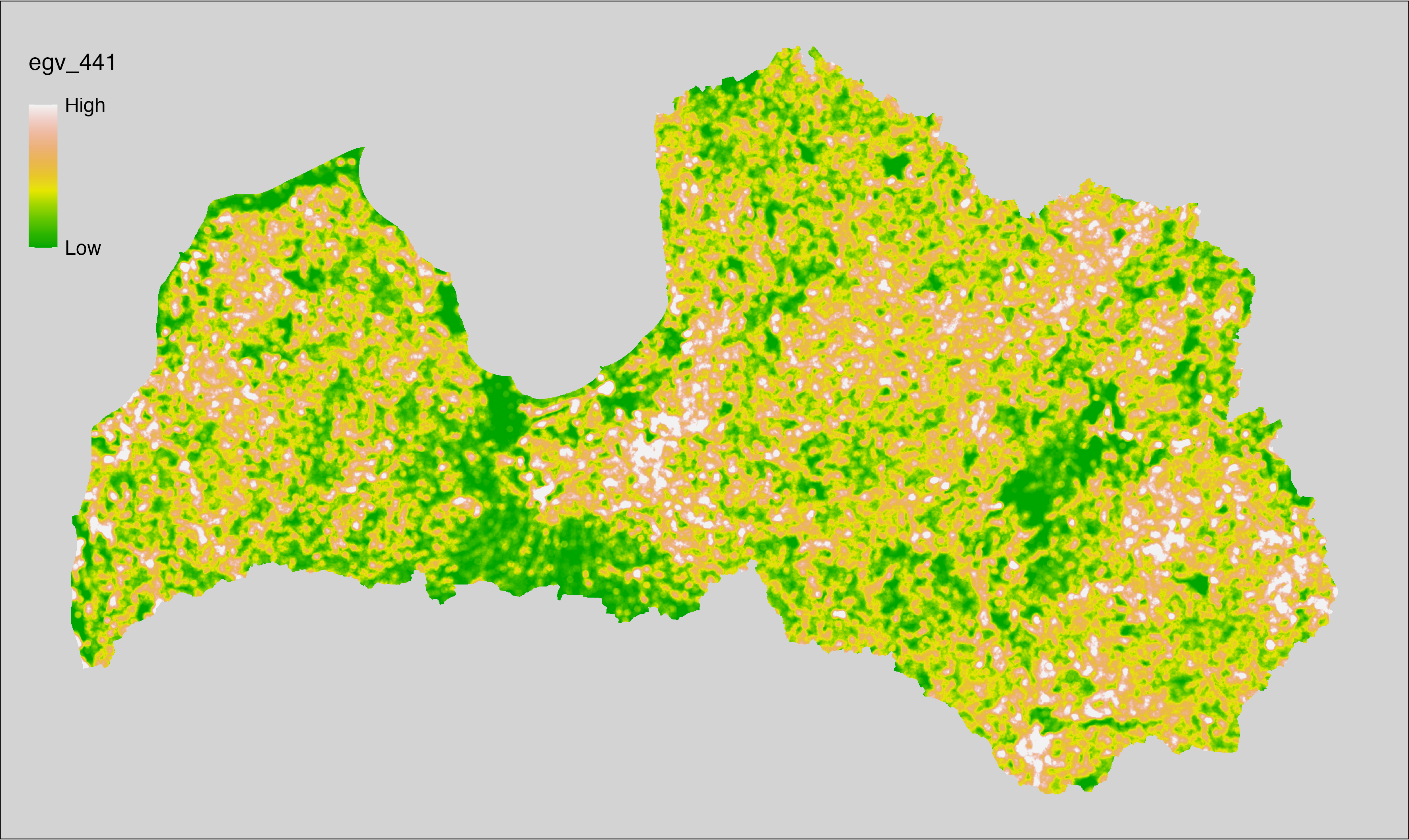
6.442 General_ShrubsOrchardsGardens_r3000
filename: General_ShrubsOrchardsGardens_r3000.tif
layername: egv_442
English name: Fractional cover of Shrubs, Young stands, Orchards, Allotment gardens within the 3 km landscape
Latvian name: Krūmāju, jaunaudžu, augļudārzu un vasarnīcu kompleksu platības īpatsvars 3 km ainavā
Procedure: The cover fraction within a radius of 3000 m around the analysis grid cell
is calculated as the area-weighted sum of the analysis cells inside
the buffer, using the workflow egvtools::radius_function(). During the calculation of the landscape
metric, inverse distance weighted (power = 2) gap filling on the output is
applied to ensure no missing values at the edges. Then the layer is
rewritten to set its name. Finally, the layer is standardised by
subtracting the arithmetic mean and dividing by the root mean squared error.
Code
# libs ----
if(!require(terra)) {install.packages("terra"); require(terra)}
if(!require(egvtools)) {remotes::install_github("aavotins/egvtools"); require(egvtools)}
# Templates -----
template100=rast("./Templates/TemplateRasters/LV100m_10km.tif")
# radii ----
radius_function(
kvadrati_path = "./Templates/TemplateGrids/tiles/",
radii_path = "./Templates/TemplateGridPoints/tiles/",
tikls100_path = "./Templates/TemplateGrids/tikls100_sauzeme.parquet",
template_path = "./Templates/TemplateRasters/LV100m_10km.tif",
input_layers = c("./RasterGrids_100m/2024/RAW/General_ShrubsOrchardsGardens_cell.tif"),
layer_prefixes = c("General_ShrubsOrchardsGardens"),
output_dir = "./RasterGrids_100m/2024/RAW/",
n_workers = 6,
radii = c("r3000"),
radius_mode = "sparse",
extract_fun = "mean",
fill_missing = TRUE,
IDW_weight = 2,
future_max_size = 40 * 1024^3)
# General_ShrubsOrchardsGardens_r3000.tif egv_442
slanis=rast("./RasterGrids_100m/2024/RAW/General_ShrubsOrchardsGardens_r3000.tif")
names(slanis)="egv_442"
slanis2=project(slanis,template100)
writeRaster(slanis2,
"./RasterGrids_100m/2024/RAW/General_ShrubsOrchardsGardens_r3000.tif",
overwrite=TRUE)
# standardisation ----
if(!require(terra)) {install.packages("terra"); require(terra)}
if(!require(tidyverse)) {install.packages("tidyverse"); require(tidyverse)}
nosaukums="General_ShrubsOrchardsGardens_r3000.tif"
ielasisanas_cels=paste0("./RasterGrids_100m/2024/RAW/",nosaukums)
saglabasanas_cels=paste0("./RasterGrids_100m/2024/Scaled/",nosaukums)
slanis=rast(ielasisanas_cels)
videjais=global(slanis,fun="mean",na.rm=TRUE)
centrets=slanis-videjais[,1]
standartnovirze=terra::global(centrets,fun="rms",na.rm=TRUE)
merogots=centrets/standartnovirze[,1]
writeRaster(merogots,
filename=saglabasanas_cels,
overwrite=TRUE)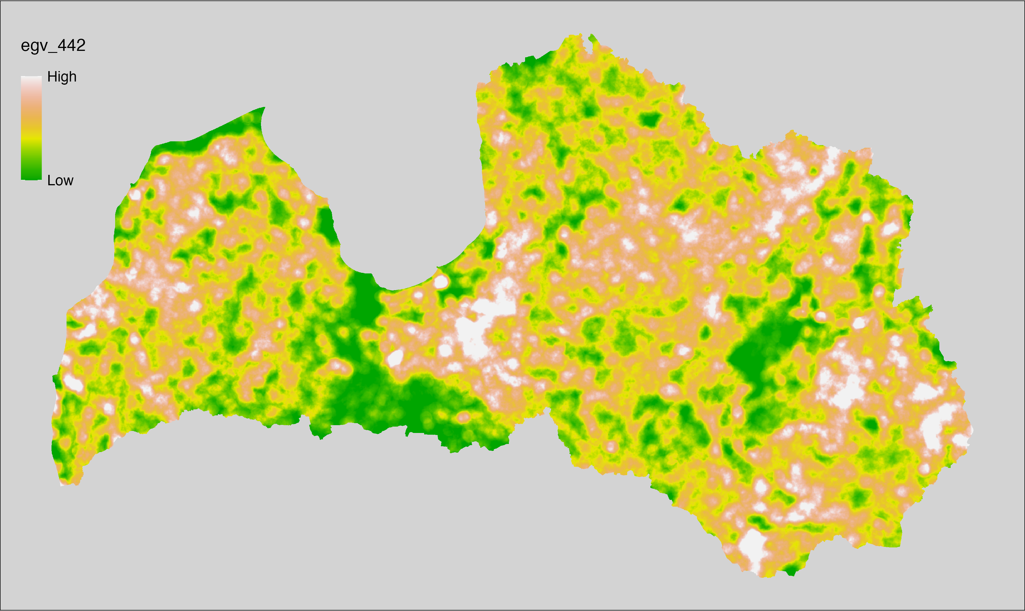
6.443 General_ShrubsOrchardsGardens_r10000
filename: General_ShrubsOrchardsGardens_r10000.tif
layername: egv_443
English name: Fractional cover of Shrubs, Young stands, Orchards, Allotment gardens within the 10 km landscape
Latvian name: Krūmāju, jaunaudžu, augļudārzu un vasarnīcu kompleksu platības īpatsvars 10 km ainavā
Procedure: The cover fraction within a radius of 10000 m around the analysis grid cell
is calculated as the area-weighted sum of the analysis cells inside
the buffer, using the workflow egvtools::radius_function(). During the calculation of the landscape
metric, inverse distance weighted (power = 2) gap filling on the output is
applied to ensure no missing values at the edges. Then the layer is
rewritten to set its name. Finally, the layer is standardised by
subtracting the arithmetic mean and dividing by the root mean squared error.
Code
# libs ----
if(!require(terra)) {install.packages("terra"); require(terra)}
if(!require(egvtools)) {remotes::install_github("aavotins/egvtools"); require(egvtools)}
# Templates -----
template100=rast("./Templates/TemplateRasters/LV100m_10km.tif")
# radii ----
radius_function(
kvadrati_path = "./Templates/TemplateGrids/tiles/",
radii_path = "./Templates/TemplateGridPoints/tiles/",
tikls100_path = "./Templates/TemplateGrids/tikls100_sauzeme.parquet",
template_path = "./Templates/TemplateRasters/LV100m_10km.tif",
input_layers = c("./RasterGrids_100m/2024/RAW/General_ShrubsOrchardsGardens_cell.tif"),
layer_prefixes = c("General_ShrubsOrchardsGardens"),
output_dir = "./RasterGrids_100m/2024/RAW/",
n_workers = 6,
radii = c("r10000"),
radius_mode = "sparse",
extract_fun = "mean",
fill_missing = TRUE,
IDW_weight = 2,
future_max_size = 40 * 1024^3)
# General_ShrubsOrchardsGardens_r10000.tif egv_443
slanis=rast("./RasterGrids_100m/2024/RAW/General_ShrubsOrchardsGardens_r10000.tif")
names(slanis)="egv_443"
slanis2=project(slanis,template100)
writeRaster(slanis2,
"./RasterGrids_100m/2024/RAW/General_ShrubsOrchardsGardens_r10000.tif",
overwrite=TRUE)
# standardisation ----
if(!require(terra)) {install.packages("terra"); require(terra)}
if(!require(tidyverse)) {install.packages("tidyverse"); require(tidyverse)}
nosaukums="General_ShrubsOrchardsGardens_r10000.tif"
ielasisanas_cels=paste0("./RasterGrids_100m/2024/RAW/",nosaukums)
saglabasanas_cels=paste0("./RasterGrids_100m/2024/Scaled/",nosaukums)
slanis=rast(ielasisanas_cels)
videjais=global(slanis,fun="mean",na.rm=TRUE)
centrets=slanis-videjais[,1]
standartnovirze=terra::global(centrets,fun="rms",na.rm=TRUE)
merogots=centrets/standartnovirze[,1]
writeRaster(merogots,
filename=saglabasanas_cels,
overwrite=TRUE)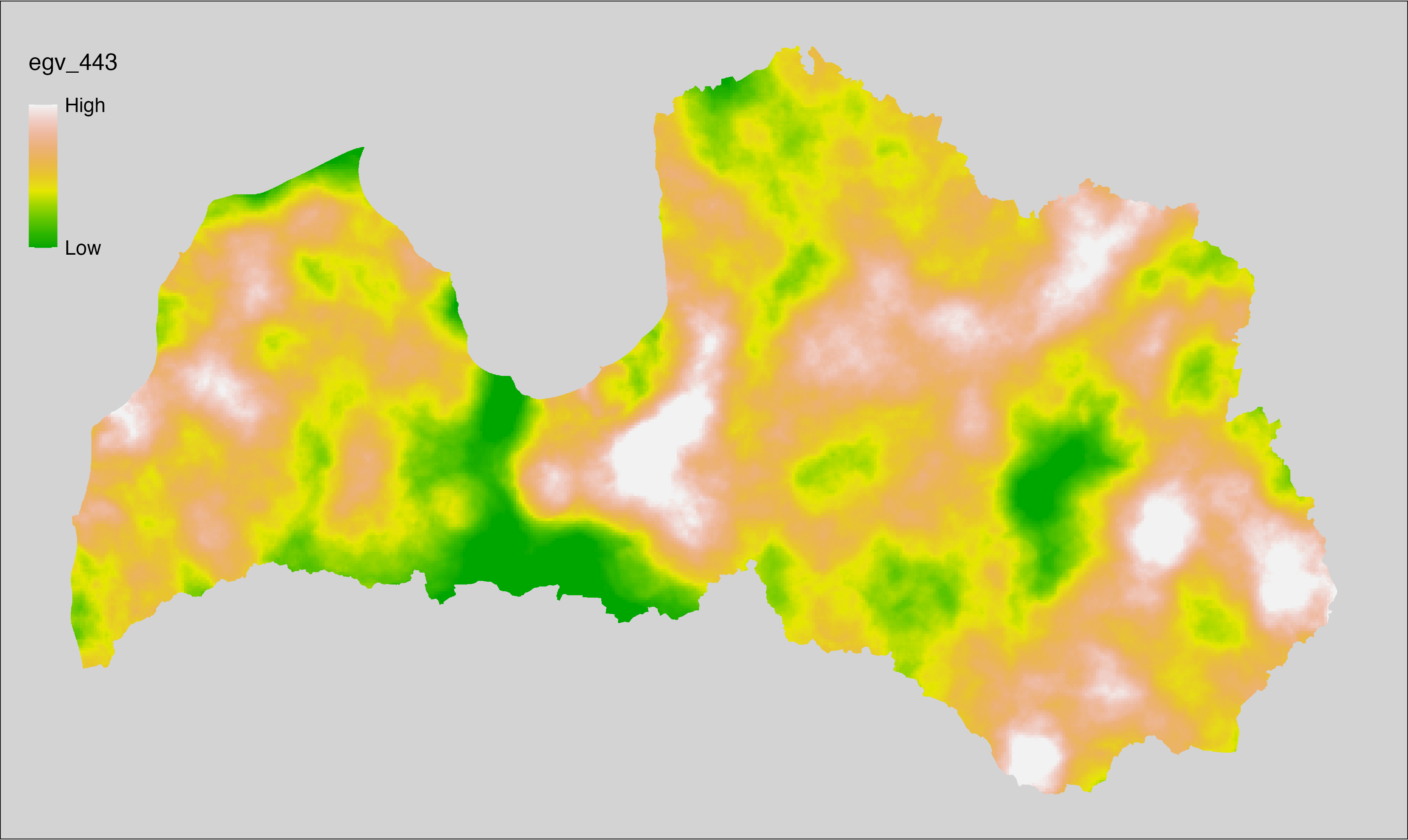
6.444 General_SwampsMiresBogsHelophytes_cell
filename: General_SwampsMiresBogsHelophytes_cell.tif
layername: egv_444
English name: Fractional cover of Swamps, Mires, Bogs, Reed-, Sedge-, Rush- Beds within the analysis cell (1 ha)
Latvian name: Purvu, niedrāju, grīslāju, meldrāju platības īpatsvars analīzes šūnā (1 ha)
Procedure: First, the swamps, mires, bogs and reed, sedge, rush beds from the
Landscape classification are selected (values between 700 and 800 are
reclassified to value 1; all others are set to 0). The resulting layer
is then aggregated to EGV resolution using the workflow egvtools::input2egv(), which
calculates the arithmetic mean to determine the cover fraction. During
aggregation, inverse distance weighted (power = 2) gap filling on the output is
applied to ensure no missing values at the edges. Finally, the layer is
standardised by subtracting the arithmetic mean and dividing by the root mean squared
error.
Code
# libs ----
if(!require(egvtools)) {remotes::install_github("aavotins/egvtools"); require(egvtools)}
if(!require(terra)) {install.packages("terra"); require(terra)}
if(!require(sf)) {install.packages("sf"); require(sf)}
if(!require(tidyverse)) {install.packages("tidyverse"); require(tidyverse)}
if(!require(sfarrow)) {install.packages("sfarrow"); require(sfarrow)}
if(!require(readxl)) {install.packages("readxl"); require(readxl)}
if(!require(raster)) {install.packages("raster"); require(raster)}
if(!require(fasterize)) {install.packages("fasterize"); require(fasterize)}
# templates ----
template100=rast("./Templates/TemplateRasters/LV100m_10km.tif")
template10=rast("./Templates/TemplateRasters/LV10m_10km.tif")
rastrs10=raster(template10)
nulls10=rast("./Templates/TemplateRasters/nulls_LV10m_10km.tif")
nulls100=rast("./Templates/TemplateRasters/nulls_LV100m_10km.tif")
# simple landscape ----
simple_landscape=rast("RasterGrids_10m/2024/Ainava_vienk_mask.tif")
# General_SwampsMiresBogsHelophytes_cell.tif egv_444 ----
purvi=ifel(simple_landscape>=700&simple_landscape<800,1,0)
i2e_rez=egvtools::input2egv(input=purvi,
egv_template= "./Templates/TemplateRasters/LV100m_10km.tif",
summary_function = "average",
missing_job = "FillOutput",
outlocation = "./RasterGrids_100m/2024/RAW/",
outfilename = "General_SwampsMiresBogsHelophytes_cell.tif",
layername = "egv_444",
idw_weight = 2,
plot_gaps = FALSE,plot_final = TRUE)
i2e_rez
rm(purvi)
rm(i2e_rez)
# standardisation ----
if(!require(terra)) {install.packages("terra"); require(terra)}
if(!require(tidyverse)) {install.packages("tidyverse"); require(tidyverse)}
nosaukums="General_SwampsMiresBogsHelophytes_cell.tif"
ielasisanas_cels=paste0("./RasterGrids_100m/2024/RAW/",nosaukums)
saglabasanas_cels=paste0("./RasterGrids_100m/2024/Scaled/",nosaukums)
slanis=rast(ielasisanas_cels)
videjais=global(slanis,fun="mean",na.rm=TRUE)
centrets=slanis-videjais[,1]
standartnovirze=terra::global(centrets,fun="rms",na.rm=TRUE)
merogots=centrets/standartnovirze[,1]
writeRaster(merogots,
filename=saglabasanas_cels,
overwrite=TRUE)
6.445 General_SwampsMiresBogsHelophytes_r500
filename: General_SwampsMiresBogsHelophytes_r500.tif
layername: egv_445
English name: Fractional cover of Swamps, Mires, Bogs, Reed-, Sedge-, Rush- Beds within the 0.5 km landscape
Latvian name: Purvu, niedrāju, grīslāju, meldrāju platības īpatsvars 0,5 km ainavā
Procedure: The cover fraction within a radius of 500 m around the analysis grid cell is
calculated as the area-weighted sum of the analysis cells inside the
buffer, using the workflow egvtools::radius_function(). During the calculation of the landscape metric,
inverse distance weighted (power = 2) gap filling on the output is applied
to ensure no missing values at the edges. Then the layer is rewritten to set
its name. Finally, the layer is standardised by subtracting the arithmetic
mean and dividing by the root mean squared error.
Code
# libs ----
if(!require(terra)) {install.packages("terra"); require(terra)}
if(!require(egvtools)) {remotes::install_github("aavotins/egvtools"); require(egvtools)}
# Templates -----
template100=rast("./Templates/TemplateRasters/LV100m_10km.tif")
# radii ----
radius_function(
kvadrati_path = "./Templates/TemplateGrids/tiles/",
radii_path = "./Templates/TemplateGridPoints/tiles/",
tikls100_path = "./Templates/TemplateGrids/tikls100_sauzeme.parquet",
template_path = "./Templates/TemplateRasters/LV100m_10km.tif",
input_layers = c("./RasterGrids_100m/2024/RAW/General_SwampsMiresBogsHelophytes_cell.tif"),
layer_prefixes = c("General_SwampsMiresBogsHelophytes"),
output_dir = "./RasterGrids_100m/2024/RAW/",
n_workers = 6,
radii = c("r500"),
radius_mode = "sparse",
extract_fun = "mean",
fill_missing = TRUE,
IDW_weight = 2,
future_max_size = 40 * 1024^3)
# General_SwampsMiresBogsHelophytes_r500.tif egv_445
slanis=rast("./RasterGrids_100m/2024/RAW/General_SwampsMiresBogsHelophytes_r500.tif")
names(slanis)="egv_445"
slanis2=project(slanis,template100)
writeRaster(slanis2,
"./RasterGrids_100m/2024/RAW/General_SwampsMiresBogsHelophytes_r500.tif",
overwrite=TRUE)
# standardisation ----
if(!require(terra)) {install.packages("terra"); require(terra)}
if(!require(tidyverse)) {install.packages("tidyverse"); require(tidyverse)}
nosaukums="General_SwampsMiresBogsHelophytes_r500.tif"
ielasisanas_cels=paste0("./RasterGrids_100m/2024/RAW/",nosaukums)
saglabasanas_cels=paste0("./RasterGrids_100m/2024/Scaled/",nosaukums)
slanis=rast(ielasisanas_cels)
videjais=global(slanis,fun="mean",na.rm=TRUE)
centrets=slanis-videjais[,1]
standartnovirze=terra::global(centrets,fun="rms",na.rm=TRUE)
merogots=centrets/standartnovirze[,1]
writeRaster(merogots,
filename=saglabasanas_cels,
overwrite=TRUE)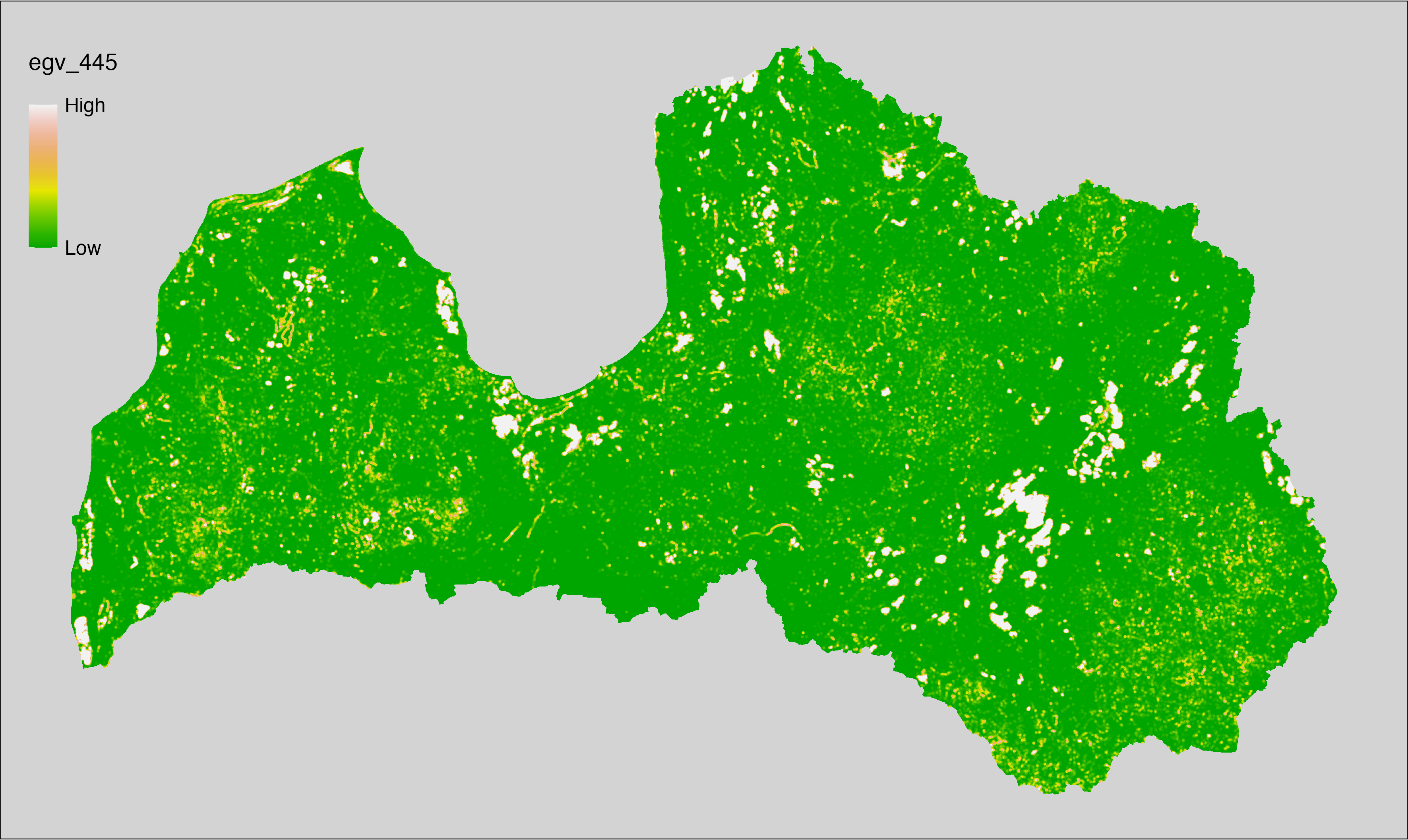
6.446 General_SwampsMiresBogsHelophytes_r1250
filename: General_SwampsMiresBogsHelophytes_r1250.tif
layername: egv_446
English name: Fractional cover of Swamps, Mires, Bogs, Reed-, Sedge-, Rush- Beds within the 1.25 km landscape
Latvian name: Purvu, niedrāju, grīslāju, meldrāju platības īpatsvars 1,25 km ainavā
Procedure: The cover fraction within a radius of 1250 m around the analysis grid cell
is calculated as the area-weighted sum of the analysis cells inside
the buffer, using the workflow egvtools::radius_function(). During the calculation of the landscape
metric, inverse distance weighted (power = 2) gap filling on the output is
applied to ensure no missing values at the edges. Then the layer is
rewritten to set its name. Finally, the layer is standardised by
subtracting the arithmetic mean and dividing by the root mean squared error.
Code
# libs ----
if(!require(terra)) {install.packages("terra"); require(terra)}
if(!require(egvtools)) {remotes::install_github("aavotins/egvtools"); require(egvtools)}
# Templates -----
template100=rast("./Templates/TemplateRasters/LV100m_10km.tif")
# radii ----
radius_function(
kvadrati_path = "./Templates/TemplateGrids/tiles/",
radii_path = "./Templates/TemplateGridPoints/tiles/",
tikls100_path = "./Templates/TemplateGrids/tikls100_sauzeme.parquet",
template_path = "./Templates/TemplateRasters/LV100m_10km.tif",
input_layers = c("./RasterGrids_100m/2024/RAW/General_SwampsMiresBogsHelophytes_cell.tif"),
layer_prefixes = c("General_SwampsMiresBogsHelophytes"),
output_dir = "./RasterGrids_100m/2024/RAW/",
n_workers = 6,
radii = c("r1250"),
radius_mode = "sparse",
extract_fun = "mean",
fill_missing = TRUE,
IDW_weight = 2,
future_max_size = 40 * 1024^3)
# General_SwampsMiresBogsHelophytes_r1250.tif egv_446
slanis=rast("./RasterGrids_100m/2024/RAW/General_SwampsMiresBogsHelophytes_r1250.tif")
names(slanis)="egv_446"
slanis2=project(slanis,template100)
writeRaster(slanis2,
"./RasterGrids_100m/2024/RAW/General_SwampsMiresBogsHelophytes_r1250.tif",
overwrite=TRUE)
# standardisation ----
if(!require(terra)) {install.packages("terra"); require(terra)}
if(!require(tidyverse)) {install.packages("tidyverse"); require(tidyverse)}
nosaukums="General_SwampsMiresBogsHelophytes_r1250.tif"
ielasisanas_cels=paste0("./RasterGrids_100m/2024/RAW/",nosaukums)
saglabasanas_cels=paste0("./RasterGrids_100m/2024/Scaled/",nosaukums)
slanis=rast(ielasisanas_cels)
videjais=global(slanis,fun="mean",na.rm=TRUE)
centrets=slanis-videjais[,1]
standartnovirze=terra::global(centrets,fun="rms",na.rm=TRUE)
merogots=centrets/standartnovirze[,1]
writeRaster(merogots,
filename=saglabasanas_cels,
overwrite=TRUE)
6.447 General_SwampsMiresBogsHelophytes_r3000
filename: General_SwampsMiresBogsHelophytes_r3000.tif
layername: egv_447
English name: Fractional cover of Swamps, Mires, Bogs, Reed-, Sedge-, Rush- Beds within the 3 km landscape
Latvian name: Purvu, niedrāju, grīslāju, meldrāju platības īpatsvars 3 km ainavā
Procedure: The cover fraction within a radius of 3000 m around the analysis grid cell
is calculated as the area-weighted sum of the analysis cells inside
the buffer, using the workflow egvtools::radius_function(). During the calculation of the landscape
metric, inverse distance weighted (power = 2) gap filling on the output is
applied to ensure no missing values at the edges. Then the layer is
rewritten to set its name. Finally, the layer is standardised by
subtracting the arithmetic mean and dividing by the root mean squared error.
Code
# libs ----
if(!require(terra)) {install.packages("terra"); require(terra)}
if(!require(egvtools)) {remotes::install_github("aavotins/egvtools"); require(egvtools)}
# Templates -----
template100=rast("./Templates/TemplateRasters/LV100m_10km.tif")
# radii ----
radius_function(
kvadrati_path = "./Templates/TemplateGrids/tiles/",
radii_path = "./Templates/TemplateGridPoints/tiles/",
tikls100_path = "./Templates/TemplateGrids/tikls100_sauzeme.parquet",
template_path = "./Templates/TemplateRasters/LV100m_10km.tif",
input_layers = c("./RasterGrids_100m/2024/RAW/General_SwampsMiresBogsHelophytes_cell.tif"),
layer_prefixes = c("General_SwampsMiresBogsHelophytes"),
output_dir = "./RasterGrids_100m/2024/RAW/",
n_workers = 6,
radii = c("r3000"),
radius_mode = "sparse",
extract_fun = "mean",
fill_missing = TRUE,
IDW_weight = 2,
future_max_size = 40 * 1024^3)
# General_SwampsMiresBogsHelophytes_r3000.tif egv_447
slanis=rast("./RasterGrids_100m/2024/RAW/General_SwampsMiresBogsHelophytes_r3000.tif")
names(slanis)="egv_447"
slanis2=project(slanis,template100)
writeRaster(slanis2,
"./RasterGrids_100m/2024/RAW/General_SwampsMiresBogsHelophytes_r3000.tif",
overwrite=TRUE)
# standardisation ----
if(!require(terra)) {install.packages("terra"); require(terra)}
if(!require(tidyverse)) {install.packages("tidyverse"); require(tidyverse)}
nosaukums="General_SwampsMiresBogsHelophytes_r3000.tif"
ielasisanas_cels=paste0("./RasterGrids_100m/2024/RAW/",nosaukums)
saglabasanas_cels=paste0("./RasterGrids_100m/2024/Scaled/",nosaukums)
slanis=rast(ielasisanas_cels)
videjais=global(slanis,fun="mean",na.rm=TRUE)
centrets=slanis-videjais[,1]
standartnovirze=terra::global(centrets,fun="rms",na.rm=TRUE)
merogots=centrets/standartnovirze[,1]
writeRaster(merogots,
filename=saglabasanas_cels,
overwrite=TRUE)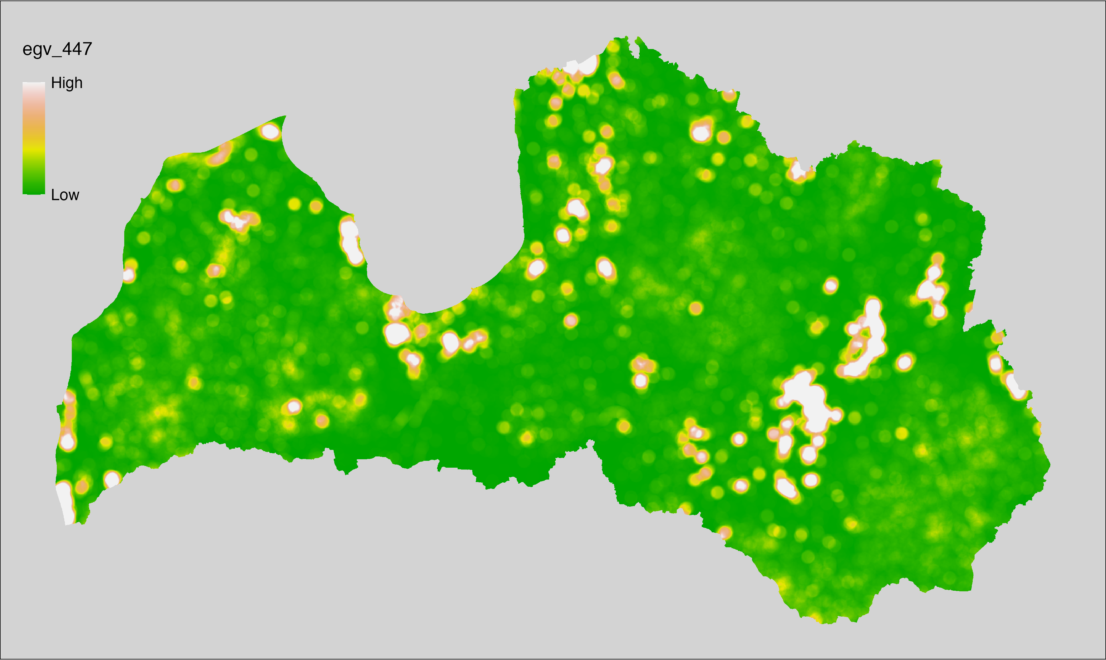
6.448 General_SwampsMiresBogsHelophytes_r10000
filename: General_SwampsMiresBogsHelophytes_r10000.tif
layername: egv_448
English name: Fractional cover of Swamps, Mires, Bogs, Reed-, Sedge-, Rush- Beds within the 10 km landscape
Latvian name: Purvu, niedrāju, grīslāju, meldrāju platības īpatsvars 10 km ainavā
Procedure: The cover fraction within a radius of 10000 m around the analysis grid cell
is calculated as the area-weighted sum of the analysis cells inside
the buffer, using the workflow egvtools::radius_function(). During the calculation of the landscape
metric, inverse distance weighted (power = 2) gap filling on the output is
applied to ensure no missing values at the edges. Then the layer is
rewritten to set its name. Finally, the layer is standardised by
subtracting the arithmetic mean and dividing by the root mean squared error.
Code
# libs ----
if(!require(terra)) {install.packages("terra"); require(terra)}
if(!require(egvtools)) {remotes::install_github("aavotins/egvtools"); require(egvtools)}
# Templates -----
template100=rast("./Templates/TemplateRasters/LV100m_10km.tif")
# radii ----
radius_function(
kvadrati_path = "./Templates/TemplateGrids/tiles/",
radii_path = "./Templates/TemplateGridPoints/tiles/",
tikls100_path = "./Templates/TemplateGrids/tikls100_sauzeme.parquet",
template_path = "./Templates/TemplateRasters/LV100m_10km.tif",
input_layers = c("./RasterGrids_100m/2024/RAW/General_SwampsMiresBogsHelophytes_cell.tif"),
layer_prefixes = c("General_SwampsMiresBogsHelophytes"),
output_dir = "./RasterGrids_100m/2024/RAW/",
n_workers = 6,
radii = c("r10000"),
radius_mode = "sparse",
extract_fun = "mean",
fill_missing = TRUE,
IDW_weight = 2,
future_max_size = 40 * 1024^3)
# General_SwampsMiresBogsHelophytes_r10000.tif egv_448
slanis=rast("./RasterGrids_100m/2024/RAW/General_SwampsMiresBogsHelophytes_r10000.tif")
names(slanis)="egv_448"
slanis2=project(slanis,template100)
writeRaster(slanis2,
"./RasterGrids_100m/2024/RAW/General_SwampsMiresBogsHelophytes_r10000.tif",
overwrite=TRUE)
# standardisation ----
if(!require(terra)) {install.packages("terra"); require(terra)}
if(!require(tidyverse)) {install.packages("tidyverse"); require(tidyverse)}
nosaukums="General_SwampsMiresBogsHelophytes_r10000.tif"
ielasisanas_cels=paste0("./RasterGrids_100m/2024/RAW/",nosaukums)
saglabasanas_cels=paste0("./RasterGrids_100m/2024/Scaled/",nosaukums)
slanis=rast(ielasisanas_cels)
videjais=global(slanis,fun="mean",na.rm=TRUE)
centrets=slanis-videjais[,1]
standartnovirze=terra::global(centrets,fun="rms",na.rm=TRUE)
merogots=centrets/standartnovirze[,1]
writeRaster(merogots,
filename=saglabasanas_cels,
overwrite=TRUE)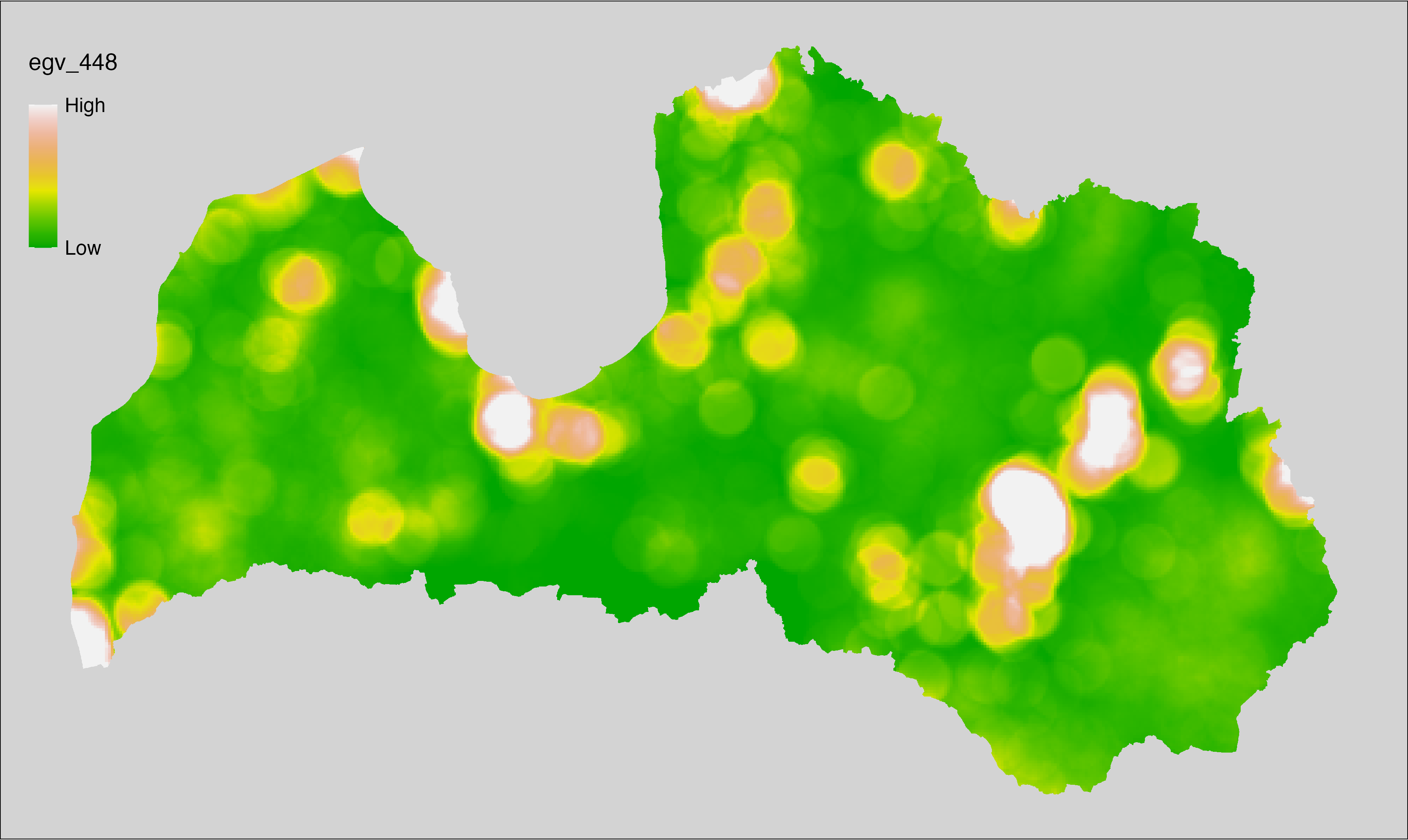
6.449 General_Trees_cell
filename: General_Trees_cell.tif
layername: egv_449
English name: Fractional cover of Trees, Shrubs, Clear-cuts within the analysis cell (1 ha)
Latvian name: Koku, krūmu un izcirtumu platības īpatsvars analīzes šūnā (1 ha)
Procedure: First, the trees, shrubs and clear cuts from the Landscape
classification are selected (values between 600 and 700 are
reclassified to value 1; all others are set to 0). The resulting layer
is then aggregated to EGV resolution using the workflow egvtools::input2egv(), which
calculates the arithmetic mean to determine the cover fraction. During
aggregation, inverse distance weighted (power = 2) gap filling on the output is
applied to ensure no missing values at the edges. Finally, the layer is
standardised by subtracting the arithmetic mean and dividing by the root mean squared
error.
Code
# libs ----
if(!require(egvtools)) {remotes::install_github("aavotins/egvtools"); require(egvtools)}
if(!require(terra)) {install.packages("terra"); require(terra)}
if(!require(sf)) {install.packages("sf"); require(sf)}
if(!require(tidyverse)) {install.packages("tidyverse"); require(tidyverse)}
if(!require(sfarrow)) {install.packages("sfarrow"); require(sfarrow)}
if(!require(readxl)) {install.packages("readxl"); require(readxl)}
if(!require(raster)) {install.packages("raster"); require(raster)}
if(!require(fasterize)) {install.packages("fasterize"); require(fasterize)}
# templates ----
template100=rast("./Templates/TemplateRasters/LV100m_10km.tif")
template10=rast("./Templates/TemplateRasters/LV10m_10km.tif")
rastrs10=raster(template10)
nulls10=rast("./Templates/TemplateRasters/nulls_LV10m_10km.tif")
nulls100=rast("./Templates/TemplateRasters/nulls_LV100m_10km.tif")
# simple landscape ----
simple_landscape=rast("RasterGrids_10m/2024/Ainava_vienk_mask.tif")
# General_Trees_cell.tif egv_449 ----
kokimezi=ifel(simple_landscape>=600&simple_landscape<700,1,0)
i2e_rez=egvtools::input2egv(input=kokimezi,
egv_template= "./Templates/TemplateRasters/LV100m_10km.tif",
summary_function = "average",
missing_job = "FillOutput",
outlocation = "./RasterGrids_100m/2024/RAW/",
outfilename = "General_Trees_cell.tif",
layername = "egv_449",
idw_weight = 2,
plot_gaps = FALSE,plot_final = TRUE)
i2e_rez
rm(kokimezi)
rm(i2e_rez)
# standardisation ----
if(!require(terra)) {install.packages("terra"); require(terra)}
if(!require(tidyverse)) {install.packages("tidyverse"); require(tidyverse)}
nosaukums="General_Trees_cell.tif"
ielasisanas_cels=paste0("./RasterGrids_100m/2024/RAW/",nosaukums)
saglabasanas_cels=paste0("./RasterGrids_100m/2024/Scaled/",nosaukums)
slanis=rast(ielasisanas_cels)
videjais=global(slanis,fun="mean",na.rm=TRUE)
centrets=slanis-videjais[,1]
standartnovirze=terra::global(centrets,fun="rms",na.rm=TRUE)
merogots=centrets/standartnovirze[,1]
writeRaster(merogots,
filename=saglabasanas_cels,
overwrite=TRUE)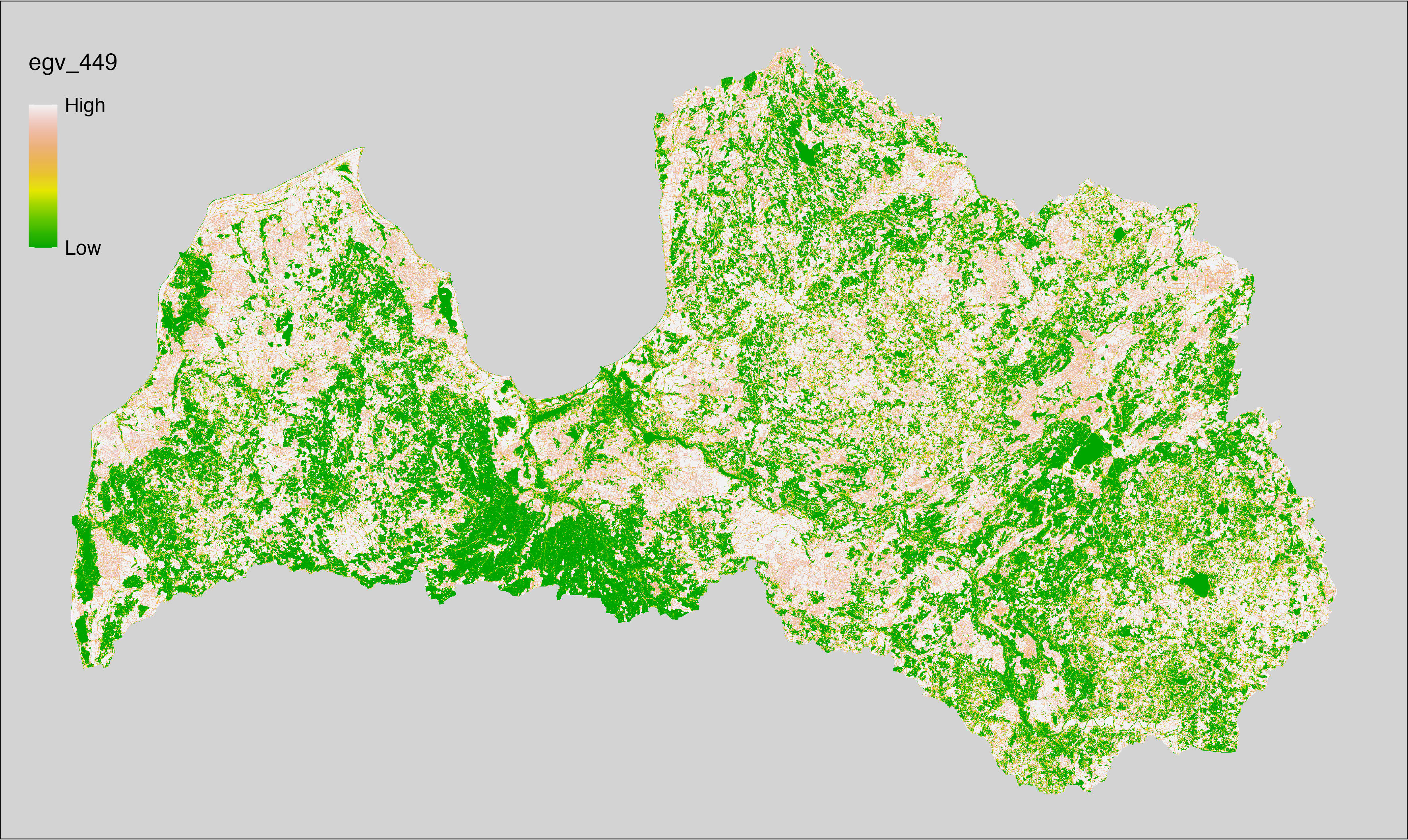
6.450 General_Trees_r500
filename: General_Trees_r500.tif
layername: egv_450
English name: Fractional cover of Trees, Shrubs, Clear-cuts within the 0.5 km landscape
Latvian name: Koku, krūmu un izcirtumu platības īpatsvars 0,5 km ainavā
Procedure: The cover fraction within a radius of 500 m around the analysis grid cell is
calculated as the area-weighted sum of the analysis cells inside the
buffer, using the workflow egvtools::radius_function(). During the calculation of the landscape metric,
inverse distance weighted (power = 2) gap filling on the output is applied
to ensure no missing values at the edges. Then the layer is rewritten to set
its name. Finally, the layer is standardised by subtracting the arithmetic
mean and dividing by the root mean squared error.
Code
# libs ----
if(!require(terra)) {install.packages("terra"); require(terra)}
if(!require(egvtools)) {remotes::install_github("aavotins/egvtools"); require(egvtools)}
# Templates -----
template100=rast("./Templates/TemplateRasters/LV100m_10km.tif")
# radii ----
radius_function(
kvadrati_path = "./Templates/TemplateGrids/tiles/",
radii_path = "./Templates/TemplateGridPoints/tiles/",
tikls100_path = "./Templates/TemplateGrids/tikls100_sauzeme.parquet",
template_path = "./Templates/TemplateRasters/LV100m_10km.tif",
input_layers = c("./RasterGrids_100m/2024/RAW/General_Trees_cell.tif"),
layer_prefixes = c("General_Trees"),
output_dir = "./RasterGrids_100m/2024/RAW/",
n_workers = 6,
radii = c("r500"),
radius_mode = "sparse",
extract_fun = "mean",
fill_missing = TRUE,
IDW_weight = 2,
future_max_size = 40 * 1024^3)
# General_Trees_r500.tif egv_450
slanis=rast("./RasterGrids_100m/2024/RAW/General_Trees_r500.tif")
names(slanis)="egv_450"
slanis2=project(slanis,template100)
writeRaster(slanis2,
"./RasterGrids_100m/2024/RAW/General_Trees_r500.tif",
overwrite=TRUE)
# standardisation ----
if(!require(terra)) {install.packages("terra"); require(terra)}
if(!require(tidyverse)) {install.packages("tidyverse"); require(tidyverse)}
nosaukums="General_Trees_r500.tif"
ielasisanas_cels=paste0("./RasterGrids_100m/2024/RAW/",nosaukums)
saglabasanas_cels=paste0("./RasterGrids_100m/2024/Scaled/",nosaukums)
slanis=rast(ielasisanas_cels)
videjais=global(slanis,fun="mean",na.rm=TRUE)
centrets=slanis-videjais[,1]
standartnovirze=terra::global(centrets,fun="rms",na.rm=TRUE)
merogots=centrets/standartnovirze[,1]
writeRaster(merogots,
filename=saglabasanas_cels,
overwrite=TRUE)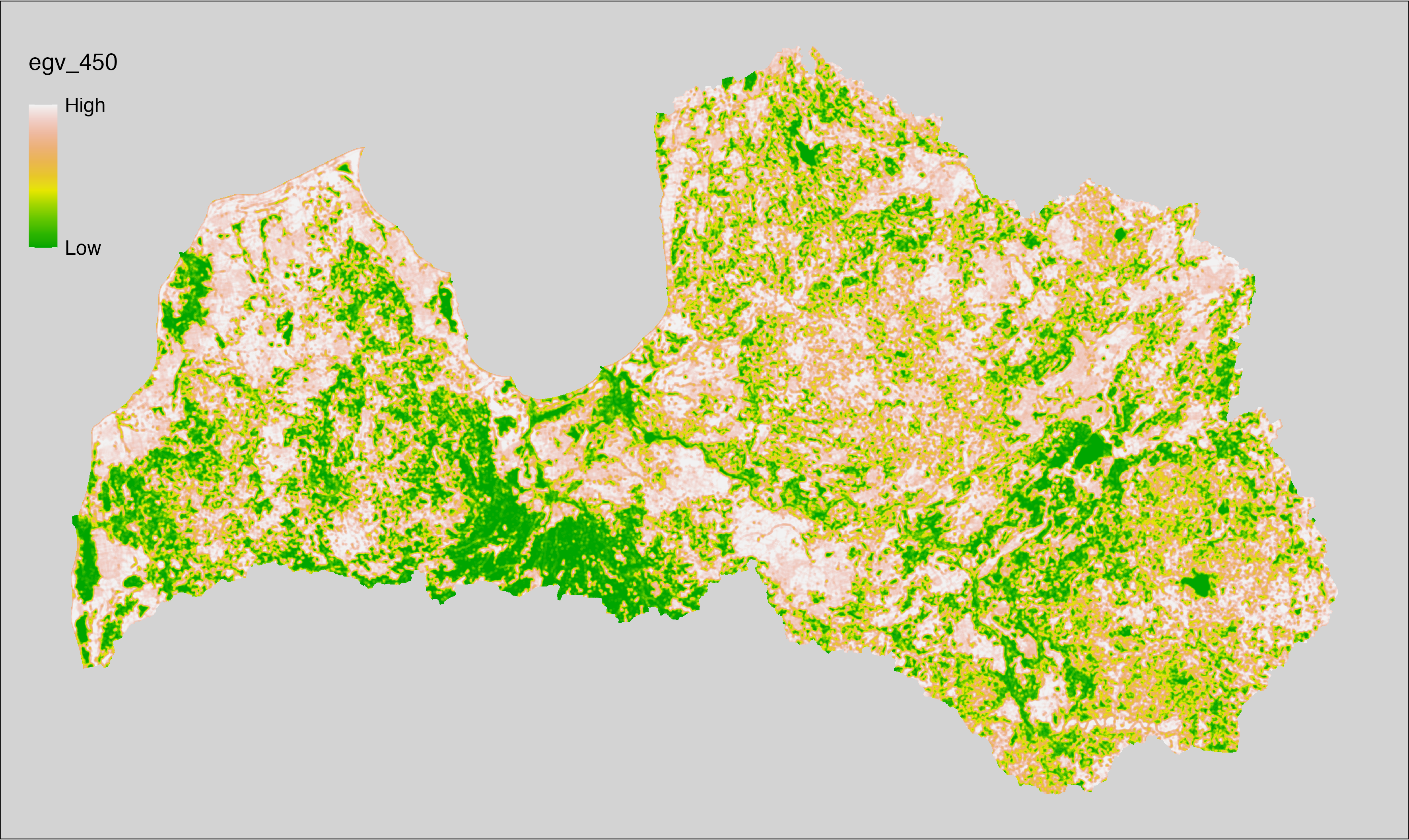
6.451 General_Trees_r1250
filename: General_Trees_r1250.tif
layername: egv_451
English name: Fractional cover of Trees, Shrubs, Clear-cuts within the 1.25 km landscape
Latvian name: Koku, krūmu un izcirtumu platības īpatsvars 1,25 km ainavā
Procedure: The cover fraction within a radius of 1250 m around the analysis grid cell
is calculated as the area-weighted sum of the analysis cells inside
the buffer, using the workflow egvtools::radius_function(). During the calculation of the landscape
metric, inverse distance weighted (power = 2) gap filling on the output is
applied to ensure no missing values at the edges. Then the layer is
rewritten to set its name. Finally, the layer is standardised by
subtracting the arithmetic mean and dividing by the root mean squared error.
Code
# libs ----
if(!require(terra)) {install.packages("terra"); require(terra)}
if(!require(egvtools)) {remotes::install_github("aavotins/egvtools"); require(egvtools)}
# Templates -----
template100=rast("./Templates/TemplateRasters/LV100m_10km.tif")
# radii ----
radius_function(
kvadrati_path = "./Templates/TemplateGrids/tiles/",
radii_path = "./Templates/TemplateGridPoints/tiles/",
tikls100_path = "./Templates/TemplateGrids/tikls100_sauzeme.parquet",
template_path = "./Templates/TemplateRasters/LV100m_10km.tif",
input_layers = c("./RasterGrids_100m/2024/RAW/General_Trees_cell.tif"),
layer_prefixes = c("General_Trees"),
output_dir = "./RasterGrids_100m/2024/RAW/",
n_workers = 6,
radii = c("r1250"),
radius_mode = "sparse",
extract_fun = "mean",
fill_missing = TRUE,
IDW_weight = 2,
future_max_size = 40 * 1024^3)
# General_Trees_r1250.tif egv_451
slanis=rast("./RasterGrids_100m/2024/RAW/General_Trees_r1250.tif")
names(slanis)="egv_451"
slanis2=project(slanis,template100)
writeRaster(slanis2,
"./RasterGrids_100m/2024/RAW/General_Trees_r1250.tif",
overwrite=TRUE)
# standardisation ----
if(!require(terra)) {install.packages("terra"); require(terra)}
if(!require(tidyverse)) {install.packages("tidyverse"); require(tidyverse)}
nosaukums="General_Trees_r1250.tif"
ielasisanas_cels=paste0("./RasterGrids_100m/2024/RAW/",nosaukums)
saglabasanas_cels=paste0("./RasterGrids_100m/2024/Scaled/",nosaukums)
slanis=rast(ielasisanas_cels)
videjais=global(slanis,fun="mean",na.rm=TRUE)
centrets=slanis-videjais[,1]
standartnovirze=terra::global(centrets,fun="rms",na.rm=TRUE)
merogots=centrets/standartnovirze[,1]
writeRaster(merogots,
filename=saglabasanas_cels,
overwrite=TRUE)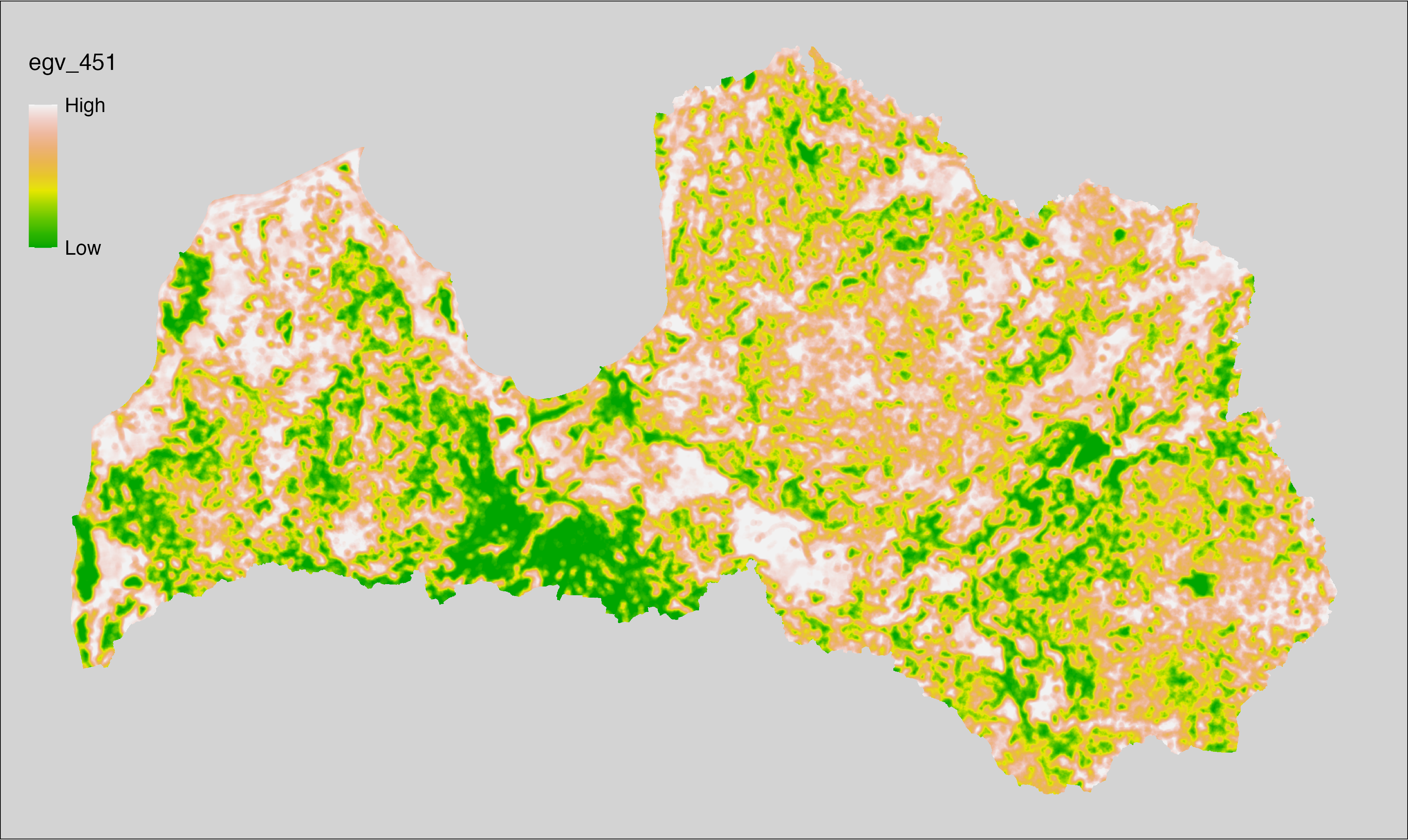
6.452 General_Trees_r3000
filename: General_Trees_r3000.tif
layername: egv_452
English name: Fractional cover of Trees, Shrubs, Clear-cuts within the 3 km landscape
Latvian name: Koku, krūmu un izcirtumu platības īpatsvars 3 km ainavā
Procedure: The cover fraction within a radius of 3000 m around the analysis grid cell
is calculated as the area-weighted sum of the analysis cells inside
the buffer, using the workflow egvtools::radius_function(). During the calculation of the landscape
metric, inverse distance weighted (power = 2) gap filling on the output is
applied to ensure no missing values at the edges. Then the layer is
rewritten to set its name. Finally, the layer is standardised by
subtracting the arithmetic mean and dividing by the root mean squared error.
Code
# libs ----
if(!require(terra)) {install.packages("terra"); require(terra)}
if(!require(egvtools)) {remotes::install_github("aavotins/egvtools"); require(egvtools)}
# Templates -----
template100=rast("./Templates/TemplateRasters/LV100m_10km.tif")
# radii ----
radius_function(
kvadrati_path = "./Templates/TemplateGrids/tiles/",
radii_path = "./Templates/TemplateGridPoints/tiles/",
tikls100_path = "./Templates/TemplateGrids/tikls100_sauzeme.parquet",
template_path = "./Templates/TemplateRasters/LV100m_10km.tif",
input_layers = c("./RasterGrids_100m/2024/RAW/General_Trees_cell.tif"),
layer_prefixes = c("General_Trees"),
output_dir = "./RasterGrids_100m/2024/RAW/",
n_workers = 6,
radii = c("r3000"),
radius_mode = "sparse",
extract_fun = "mean",
fill_missing = TRUE,
IDW_weight = 2,
future_max_size = 40 * 1024^3)
# General_Trees_r3000.tif egv_452
slanis=rast("./RasterGrids_100m/2024/RAW/General_Trees_r3000.tif")
names(slanis)="egv_452"
slanis2=project(slanis,template100)
writeRaster(slanis2,
"./RasterGrids_100m/2024/RAW/General_Trees_r3000.tif",
overwrite=TRUE)
# standardisation ----
if(!require(terra)) {install.packages("terra"); require(terra)}
if(!require(tidyverse)) {install.packages("tidyverse"); require(tidyverse)}
nosaukums="General_Trees_r3000.tif"
ielasisanas_cels=paste0("./RasterGrids_100m/2024/RAW/",nosaukums)
saglabasanas_cels=paste0("./RasterGrids_100m/2024/Scaled/",nosaukums)
slanis=rast(ielasisanas_cels)
videjais=global(slanis,fun="mean",na.rm=TRUE)
centrets=slanis-videjais[,1]
standartnovirze=terra::global(centrets,fun="rms",na.rm=TRUE)
merogots=centrets/standartnovirze[,1]
writeRaster(merogots,
filename=saglabasanas_cels,
overwrite=TRUE)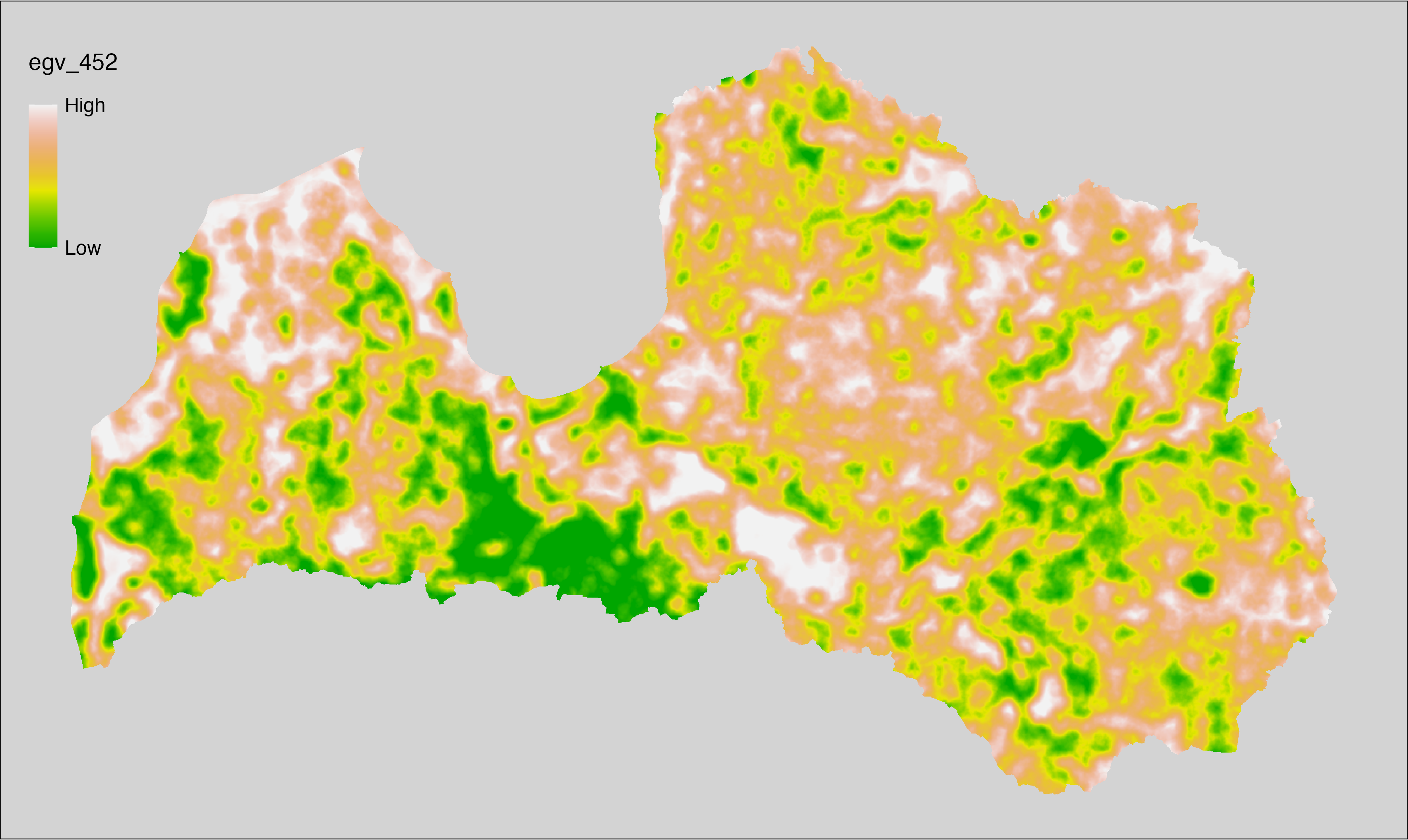
6.453 General_Trees_r10000
filename: General_Trees_r10000.tif
layername: egv_453
English name: Fractional cover of Trees, Shrubs, Clear-cuts within the 10 km landscape
Latvian name: Koku, krūmu un izcirtumu platības īpatsvars 10 km ainavā
Procedure: The cover fraction within a radius of 10000 m around the analysis grid cell
is calculated as the area-weighted sum of the analysis cells inside
the buffer, using the workflow egvtools::radius_function(). During the calculation of the landscape
metric, inverse distance weighted (power = 2) gap filling on the output is
applied to ensure no missing values at the edges. Then the layer is
rewritten to set its name. Finally, the layer is standardised by
subtracting the arithmetic mean and dividing by the root mean squared error.
Code
# libs ----
if(!require(terra)) {install.packages("terra"); require(terra)}
if(!require(egvtools)) {remotes::install_github("aavotins/egvtools"); require(egvtools)}
# Templates -----
template100=rast("./Templates/TemplateRasters/LV100m_10km.tif")
# radii ----
radius_function(
kvadrati_path = "./Templates/TemplateGrids/tiles/",
radii_path = "./Templates/TemplateGridPoints/tiles/",
tikls100_path = "./Templates/TemplateGrids/tikls100_sauzeme.parquet",
template_path = "./Templates/TemplateRasters/LV100m_10km.tif",
input_layers = c("./RasterGrids_100m/2024/RAW/General_Trees_cell.tif"),
layer_prefixes = c("General_Trees"),
output_dir = "./RasterGrids_100m/2024/RAW/",
n_workers = 6,
radii = c("r10000"),
radius_mode = "sparse",
extract_fun = "mean",
fill_missing = TRUE,
IDW_weight = 2,
future_max_size = 40 * 1024^3)
# General_Trees_r10000.tif egv_453
slanis=rast("./RasterGrids_100m/2024/RAW/General_Trees_r10000.tif")
names(slanis)="egv_453"
slanis2=project(slanis,template100)
writeRaster(slanis2,
"./RasterGrids_100m/2024/RAW/General_Trees_r10000.tif",
overwrite=TRUE)
# standardisation ----
if(!require(terra)) {install.packages("terra"); require(terra)}
if(!require(tidyverse)) {install.packages("tidyverse"); require(tidyverse)}
nosaukums="General_Trees_r10000.tif"
ielasisanas_cels=paste0("./RasterGrids_100m/2024/RAW/",nosaukums)
saglabasanas_cels=paste0("./RasterGrids_100m/2024/Scaled/",nosaukums)
slanis=rast(ielasisanas_cels)
videjais=global(slanis,fun="mean",na.rm=TRUE)
centrets=slanis-videjais[,1]
standartnovirze=terra::global(centrets,fun="rms",na.rm=TRUE)
merogots=centrets/standartnovirze[,1]
writeRaster(merogots,
filename=saglabasanas_cels,
overwrite=TRUE)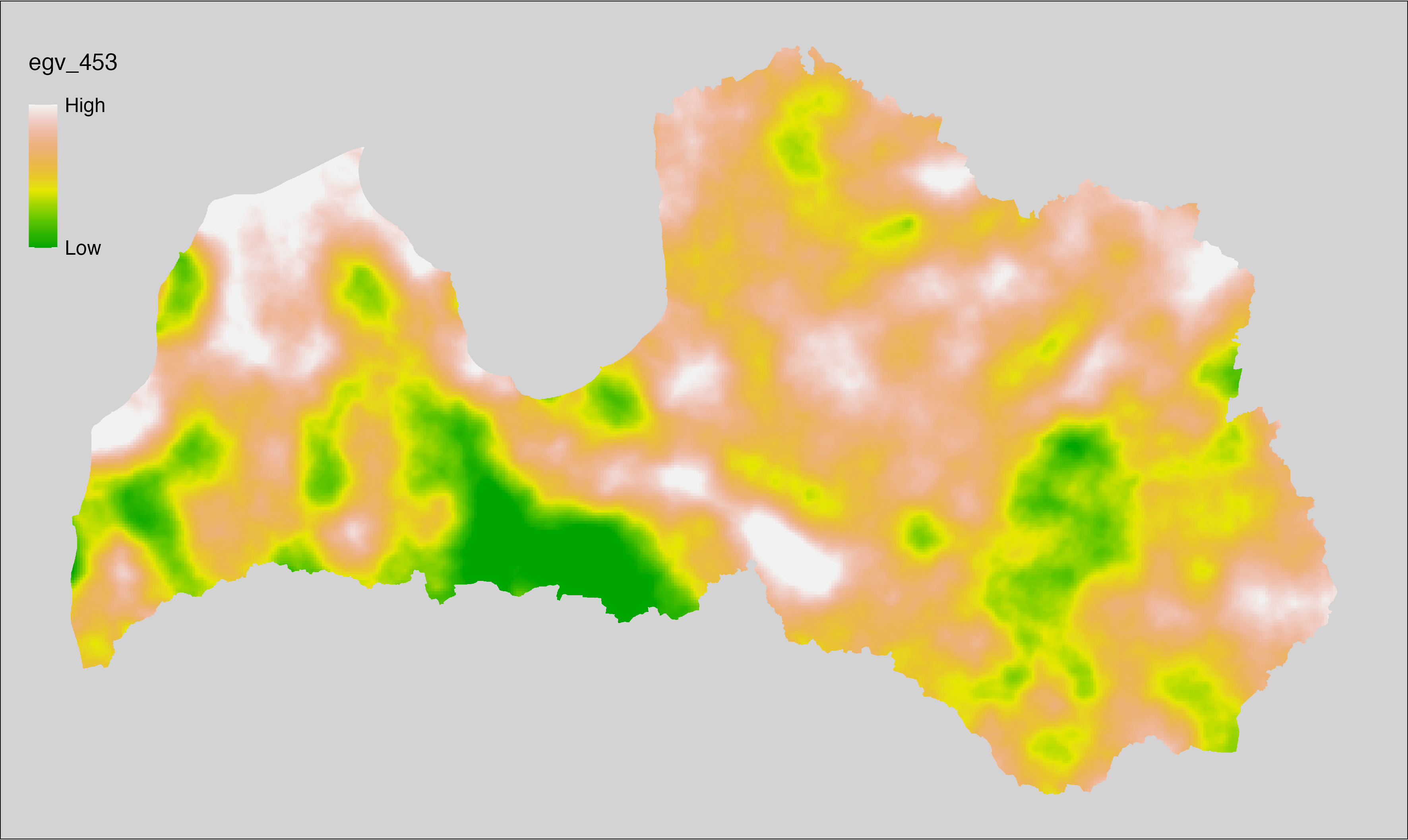
6.454 General_TreesOutsideForests_cell
filename: General_TreesOutsideForests_cell.tif
layername: egv_454
English name: Fractional cover of Tree covered areas Outside Forests within the analysis cell (1 ha)
Latvian name: Ar kokiem klāto teritoriju ārpus mežiem platības īpatsvars analīzes šūnā (1 ha)
Procedure: First, the tree covered areas outside forest stands from the Landscape
classification are selected (value 640 is reclassified to value 1;
all others are set to 0). The resulting layer
is then aggregated to EGV resolution using the workflow egvtools::input2egv(), which
calculates the arithmetic mean to determine the cover fraction. During
aggregation, inverse distance weighted (power = 2) gap filling on the output is
applied to ensure no missing values at the edges. Finally, the layer is
standardised by subtracting the arithmetic mean and dividing by the root mean squared
error.
Code
# libs ----
if(!require(egvtools)) {remotes::install_github("aavotins/egvtools"); require(egvtools)}
if(!require(terra)) {install.packages("terra"); require(terra)}
if(!require(sf)) {install.packages("sf"); require(sf)}
if(!require(tidyverse)) {install.packages("tidyverse"); require(tidyverse)}
if(!require(sfarrow)) {install.packages("sfarrow"); require(sfarrow)}
if(!require(readxl)) {install.packages("readxl"); require(readxl)}
if(!require(raster)) {install.packages("raster"); require(raster)}
if(!require(fasterize)) {install.packages("fasterize"); require(fasterize)}
# templates ----
template100=rast("./Templates/TemplateRasters/LV100m_10km.tif")
template10=rast("./Templates/TemplateRasters/LV10m_10km.tif")
rastrs10=raster(template10)
nulls10=rast("./Templates/TemplateRasters/nulls_LV10m_10km.tif")
nulls100=rast("./Templates/TemplateRasters/nulls_LV100m_10km.tif")
# simple landscape ----
simple_landscape=rast("RasterGrids_10m/2024/Ainava_vienk_mask.tif")
# General_TreesOutsideForests_cell.tif egv_454 ----
kokiarpuse=ifel(simple_landscape==640,1,0)
i2e_rez=egvtools::input2egv(input=kokiarpuse,
egv_template= "./Templates/TemplateRasters/LV100m_10km.tif",
summary_function = "average",
missing_job = "FillOutput",
outlocation = "./RasterGrids_100m/2024/RAW/",
outfilename = "General_TreesOutsideForests_cell.tif",
layername = "egv_454",
idw_weight = 2,
plot_gaps = FALSE,plot_final = TRUE)
i2e_rez
rm(kokiarpuse)
rm(i2e_rez)
# standardisation ----
if(!require(terra)) {install.packages("terra"); require(terra)}
if(!require(tidyverse)) {install.packages("tidyverse"); require(tidyverse)}
nosaukums="General_TreesOutsideForests_cell.tif"
ielasisanas_cels=paste0("./RasterGrids_100m/2024/RAW/",nosaukums)
saglabasanas_cels=paste0("./RasterGrids_100m/2024/Scaled/",nosaukums)
slanis=rast(ielasisanas_cels)
videjais=global(slanis,fun="mean",na.rm=TRUE)
centrets=slanis-videjais[,1]
standartnovirze=terra::global(centrets,fun="rms",na.rm=TRUE)
merogots=centrets/standartnovirze[,1]
writeRaster(merogots,
filename=saglabasanas_cels,
overwrite=TRUE)
6.455 General_TreesOutsideForests_r500
filename: General_TreesOutsideForests_r500.tif
layername: egv_455
English name: Fractional cover of Tree covered areas Outside Forests within the 0.5 km landscape
Latvian name: Ar kokiem klāto teritoriju ārpus mežiem platības īpatsvars 0,5 km ainavā
Procedure: The cover fraction within a radius of 500 m around the analysis grid cell is
calculated as the area-weighted sum of the analysis cells inside the
buffer, using the workflow egvtools::radius_function(). During the calculation of the landscape metric,
inverse distance weighted (power = 2) gap filling on the output is applied
to ensure no missing values at the edges. Then the layer is rewritten to set
its name. Finally, the layer is standardised by subtracting the arithmetic
mean and dividing by the root mean squared error.
Code
# libs ----
if(!require(terra)) {install.packages("terra"); require(terra)}
if(!require(egvtools)) {remotes::install_github("aavotins/egvtools"); require(egvtools)}
# Templates -----
template100=rast("./Templates/TemplateRasters/LV100m_10km.tif")
# radii ----
radius_function(
kvadrati_path = "./Templates/TemplateGrids/tiles/",
radii_path = "./Templates/TemplateGridPoints/tiles/",
tikls100_path = "./Templates/TemplateGrids/tikls100_sauzeme.parquet",
template_path = "./Templates/TemplateRasters/LV100m_10km.tif",
input_layers = c("./RasterGrids_100m/2024/RAW/General_TreesOutsideForests_cell.tif"),
layer_prefixes = c("General_TreesOutsideForests"),
output_dir = "./RasterGrids_100m/2024/RAW/",
n_workers = 6,
radii = c("r500"),
radius_mode = "sparse",
extract_fun = "mean",
fill_missing = TRUE,
IDW_weight = 2,
future_max_size = 40 * 1024^3)
# General_TreesOutsideForests_r500.tif egv_455
slanis=rast("./RasterGrids_100m/2024/RAW/General_TreesOutsideForests_r500.tif")
names(slanis)="egv_455"
slanis2=project(slanis,template100)
writeRaster(slanis2,
"./RasterGrids_100m/2024/RAW/General_TreesOutsideForests_r500.tif",
overwrite=TRUE)
# standardisation ----
if(!require(terra)) {install.packages("terra"); require(terra)}
if(!require(tidyverse)) {install.packages("tidyverse"); require(tidyverse)}
nosaukums="General_TreesOutsideForests_r500.tif"
ielasisanas_cels=paste0("./RasterGrids_100m/2024/RAW/",nosaukums)
saglabasanas_cels=paste0("./RasterGrids_100m/2024/Scaled/",nosaukums)
slanis=rast(ielasisanas_cels)
videjais=global(slanis,fun="mean",na.rm=TRUE)
centrets=slanis-videjais[,1]
standartnovirze=terra::global(centrets,fun="rms",na.rm=TRUE)
merogots=centrets/standartnovirze[,1]
writeRaster(merogots,
filename=saglabasanas_cels,
overwrite=TRUE)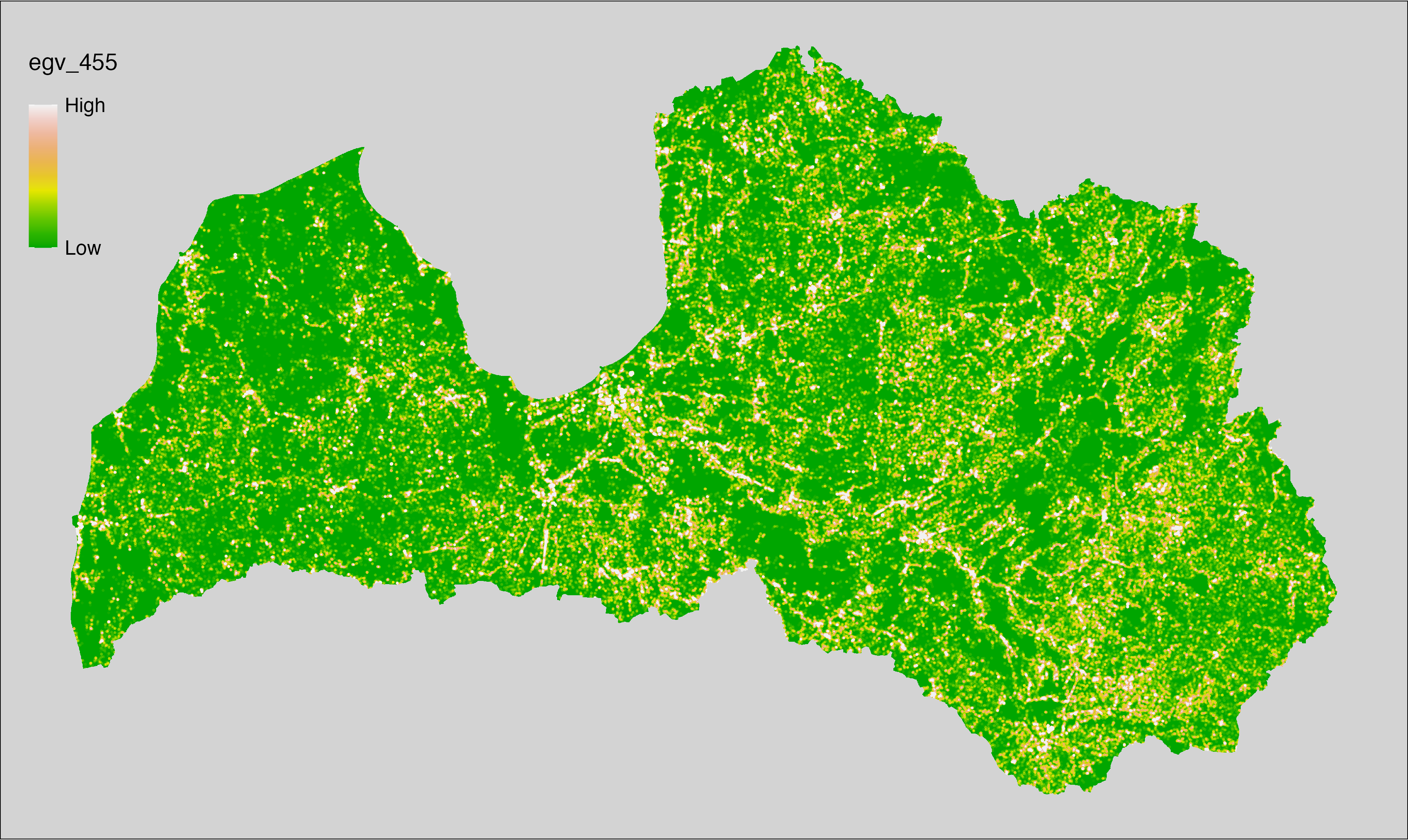
6.456 General_TreesOutsideForests_r1250
filename: General_TreesOutsideForests_r1250.tif
layername: egv_456
English name: Fractional cover of Tree covered areas Outside Forests within the 1.25 km landscape
Latvian name: Ar kokiem klāto teritoriju ārpus mežiem platības īpatsvars 1,25 km ainavā
Procedure: The cover fraction within a radius of 1250 m around the analysis grid cell
is calculated as the area-weighted sum of the analysis cells inside
the buffer, using the workflow egvtools::radius_function(). During the calculation of the landscape
metric, inverse distance weighted (power = 2) gap filling on the output is
applied to ensure no missing values at the edges. Then the layer is
rewritten to set its name. Finally, the layer is standardised by
subtracting the arithmetic mean and dividing by the root mean squared error.
Code
# libs ----
if(!require(terra)) {install.packages("terra"); require(terra)}
if(!require(egvtools)) {remotes::install_github("aavotins/egvtools"); require(egvtools)}
# Templates -----
template100=rast("./Templates/TemplateRasters/LV100m_10km.tif")
# radii ----
radius_function(
kvadrati_path = "./Templates/TemplateGrids/tiles/",
radii_path = "./Templates/TemplateGridPoints/tiles/",
tikls100_path = "./Templates/TemplateGrids/tikls100_sauzeme.parquet",
template_path = "./Templates/TemplateRasters/LV100m_10km.tif",
input_layers = c("./RasterGrids_100m/2024/RAW/General_TreesOutsideForests_cell.tif"),
layer_prefixes = c("General_TreesOutsideForests"),
output_dir = "./RasterGrids_100m/2024/RAW/",
n_workers = 6,
radii = c("r1250"),
radius_mode = "sparse",
extract_fun = "mean",
fill_missing = TRUE,
IDW_weight = 2,
future_max_size = 40 * 1024^3)
# General_TreesOutsideForests_r1250.tif egv_456
slanis=rast("./RasterGrids_100m/2024/RAW/General_TreesOutsideForests_r1250.tif")
names(slanis)="egv_456"
slanis2=project(slanis,template100)
writeRaster(slanis2,
"./RasterGrids_100m/2024/RAW/General_TreesOutsideForests_r1250.tif",
overwrite=TRUE)
# standardisation ----
if(!require(terra)) {install.packages("terra"); require(terra)}
if(!require(tidyverse)) {install.packages("tidyverse"); require(tidyverse)}
nosaukums="General_TreesOutsideForests_r1250.tif"
ielasisanas_cels=paste0("./RasterGrids_100m/2024/RAW/",nosaukums)
saglabasanas_cels=paste0("./RasterGrids_100m/2024/Scaled/",nosaukums)
slanis=rast(ielasisanas_cels)
videjais=global(slanis,fun="mean",na.rm=TRUE)
centrets=slanis-videjais[,1]
standartnovirze=terra::global(centrets,fun="rms",na.rm=TRUE)
merogots=centrets/standartnovirze[,1]
writeRaster(merogots,
filename=saglabasanas_cels,
overwrite=TRUE)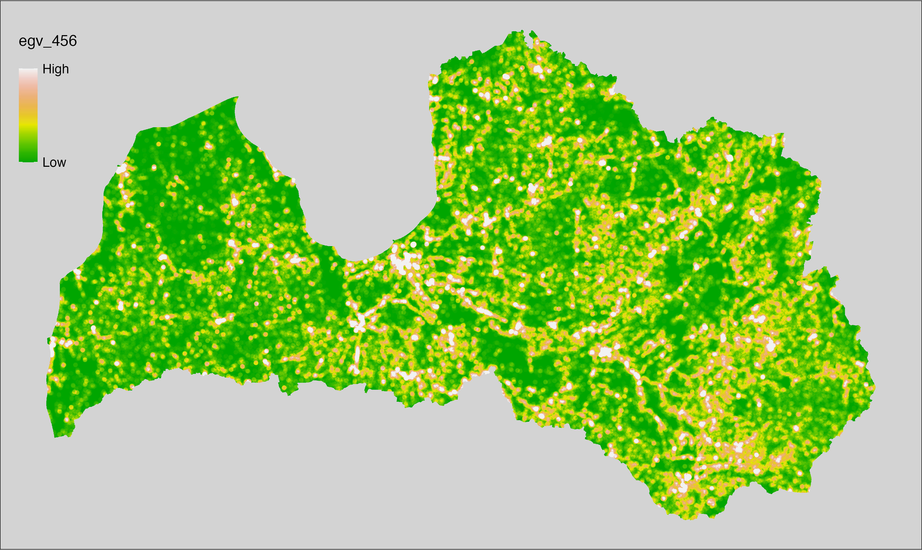
6.457 General_TreesOutsideForests_r3000
filename: General_TreesOutsideForests_r3000.tif
layername: egv_457
English name: Fractional cover of Tree covered areas Outside Forests within the 3 km landscape
Latvian name: Ar kokiem klāto teritoriju ārpus mežiem platības īpatsvars 3 km ainavā
Procedure: The cover fraction within a radius of 3000 m around the analysis grid cell
is calculated as the area-weighted sum of the analysis cells inside
the buffer, using the workflow egvtools::radius_function(). During the calculation of the landscape
metric, inverse distance weighted (power = 2) gap filling on the output is
applied to ensure no missing values at the edges. Then the layer is
rewritten to set its name. Finally, the layer is standardised by
subtracting the arithmetic mean and dividing by the root mean squared error.
Code
# libs ----
if(!require(terra)) {install.packages("terra"); require(terra)}
if(!require(egvtools)) {remotes::install_github("aavotins/egvtools"); require(egvtools)}
# Templates -----
template100=rast("./Templates/TemplateRasters/LV100m_10km.tif")
# radii ----
radius_function(
kvadrati_path = "./Templates/TemplateGrids/tiles/",
radii_path = "./Templates/TemplateGridPoints/tiles/",
tikls100_path = "./Templates/TemplateGrids/tikls100_sauzeme.parquet",
template_path = "./Templates/TemplateRasters/LV100m_10km.tif",
input_layers = c("./RasterGrids_100m/2024/RAW/General_TreesOutsideForests_cell.tif"),
layer_prefixes = c("General_TreesOutsideForests"),
output_dir = "./RasterGrids_100m/2024/RAW/",
n_workers = 6,
radii = c("r3000"),
radius_mode = "sparse",
extract_fun = "mean",
fill_missing = TRUE,
IDW_weight = 2,
future_max_size = 40 * 1024^3)
# General_TreesOutsideForests_r3000.tif egv_457
slanis=rast("./RasterGrids_100m/2024/RAW/General_TreesOutsideForests_r3000.tif")
names(slanis)="egv_457"
slanis2=project(slanis,template100)
writeRaster(slanis2,
"./RasterGrids_100m/2024/RAW/General_TreesOutsideForests_r3000.tif",
overwrite=TRUE)
# standardisation ----
if(!require(terra)) {install.packages("terra"); require(terra)}
if(!require(tidyverse)) {install.packages("tidyverse"); require(tidyverse)}
nosaukums="General_TreesOutsideForests_r3000.tif"
ielasisanas_cels=paste0("./RasterGrids_100m/2024/RAW/",nosaukums)
saglabasanas_cels=paste0("./RasterGrids_100m/2024/Scaled/",nosaukums)
slanis=rast(ielasisanas_cels)
videjais=global(slanis,fun="mean",na.rm=TRUE)
centrets=slanis-videjais[,1]
standartnovirze=terra::global(centrets,fun="rms",na.rm=TRUE)
merogots=centrets/standartnovirze[,1]
writeRaster(merogots,
filename=saglabasanas_cels,
overwrite=TRUE)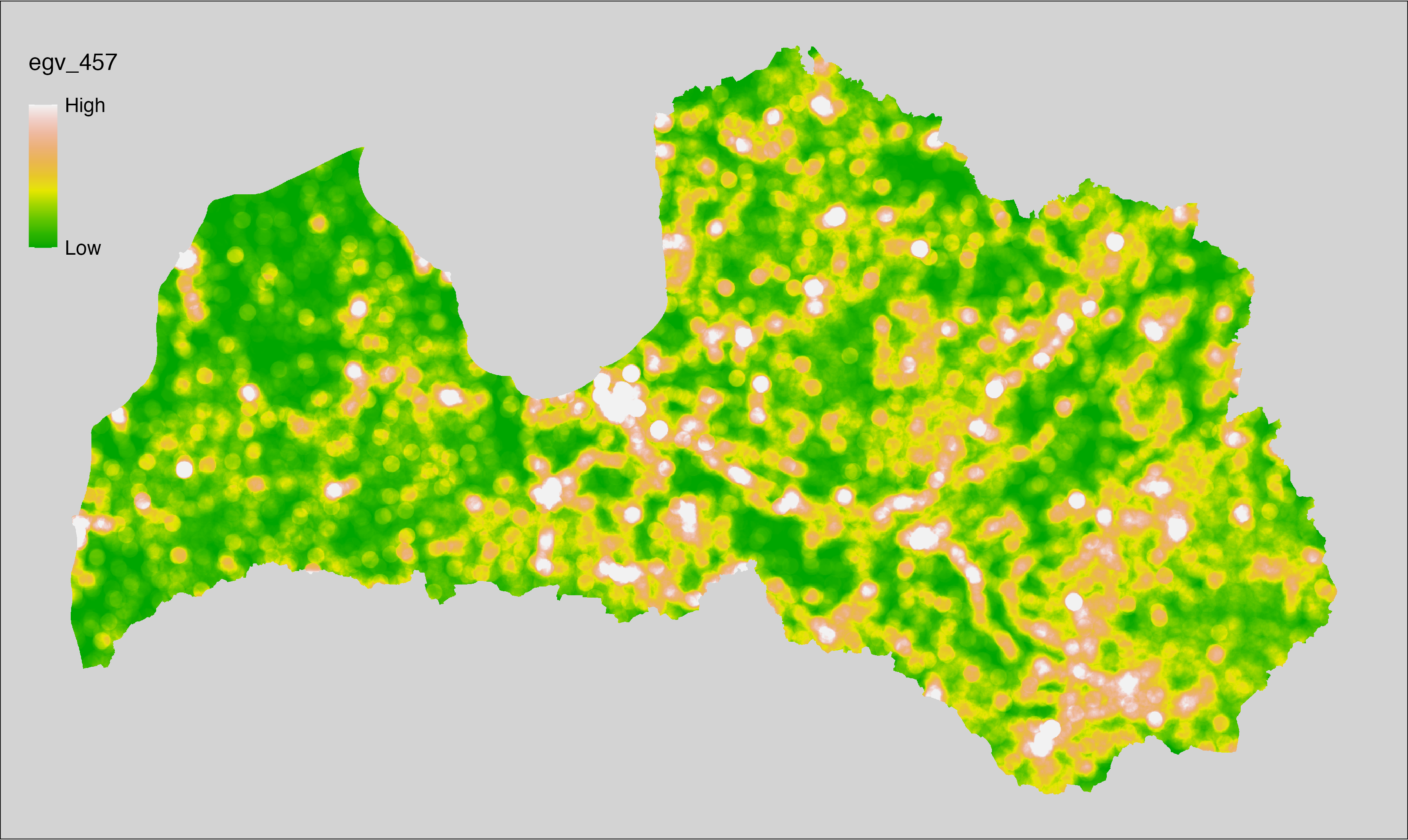
6.458 General_TreesOutsideForests_r10000
filename: General_TreesOutsideForests_r10000.tif
layername: egv_458
English name: Fractional cover of Tree covered areas Outside Forests within the 10 km landscape
Latvian name: Ar kokiem klāto teritoriju ārpus mežiem platības īpatsvars 10 km ainavā
Procedure: The cover fraction within a radius of 10000 m around the analysis grid cell
is calculated as the area-weighted sum of the analysis cells inside
the buffer, using the workflow egvtools::radius_function(). During the calculation of the landscape
metric, inverse distance weighted (power = 2) gap filling on the output is
applied to ensure no missing values at the edges. Then the layer is
rewritten to set its name. Finally, the layer is standardised by
subtracting the arithmetic mean and dividing by the root mean squared error.
Code
# libs ----
if(!require(terra)) {install.packages("terra"); require(terra)}
if(!require(egvtools)) {remotes::install_github("aavotins/egvtools"); require(egvtools)}
# Templates -----
template100=rast("./Templates/TemplateRasters/LV100m_10km.tif")
# radii ----
radius_function(
kvadrati_path = "./Templates/TemplateGrids/tiles/",
radii_path = "./Templates/TemplateGridPoints/tiles/",
tikls100_path = "./Templates/TemplateGrids/tikls100_sauzeme.parquet",
template_path = "./Templates/TemplateRasters/LV100m_10km.tif",
input_layers = c("./RasterGrids_100m/2024/RAW/General_TreesOutsideForests_cell.tif"),
layer_prefixes = c("General_TreesOutsideForests"),
output_dir = "./RasterGrids_100m/2024/RAW/",
n_workers = 6,
radii = c("r10000"),
radius_mode = "sparse",
extract_fun = "mean",
fill_missing = TRUE,
IDW_weight = 2,
future_max_size = 40 * 1024^3)
# General_TreesOutsideForests_r10000.tif egv_458
slanis=rast("./RasterGrids_100m/2024/RAW/General_TreesOutsideForests_r10000.tif")
names(slanis)="egv_458"
slanis2=project(slanis,template100)
writeRaster(slanis2,
"./RasterGrids_100m/2024/RAW/General_TreesOutsideForests_r10000.tif",
overwrite=TRUE)
# standardisation ----
if(!require(terra)) {install.packages("terra"); require(terra)}
if(!require(tidyverse)) {install.packages("tidyverse"); require(tidyverse)}
nosaukums="General_TreesOutsideForests_r10000.tif"
ielasisanas_cels=paste0("./RasterGrids_100m/2024/RAW/",nosaukums)
saglabasanas_cels=paste0("./RasterGrids_100m/2024/Scaled/",nosaukums)
slanis=rast(ielasisanas_cels)
videjais=global(slanis,fun="mean",na.rm=TRUE)
centrets=slanis-videjais[,1]
standartnovirze=terra::global(centrets,fun="rms",na.rm=TRUE)
merogots=centrets/standartnovirze[,1]
writeRaster(merogots,
filename=saglabasanas_cels,
overwrite=TRUE)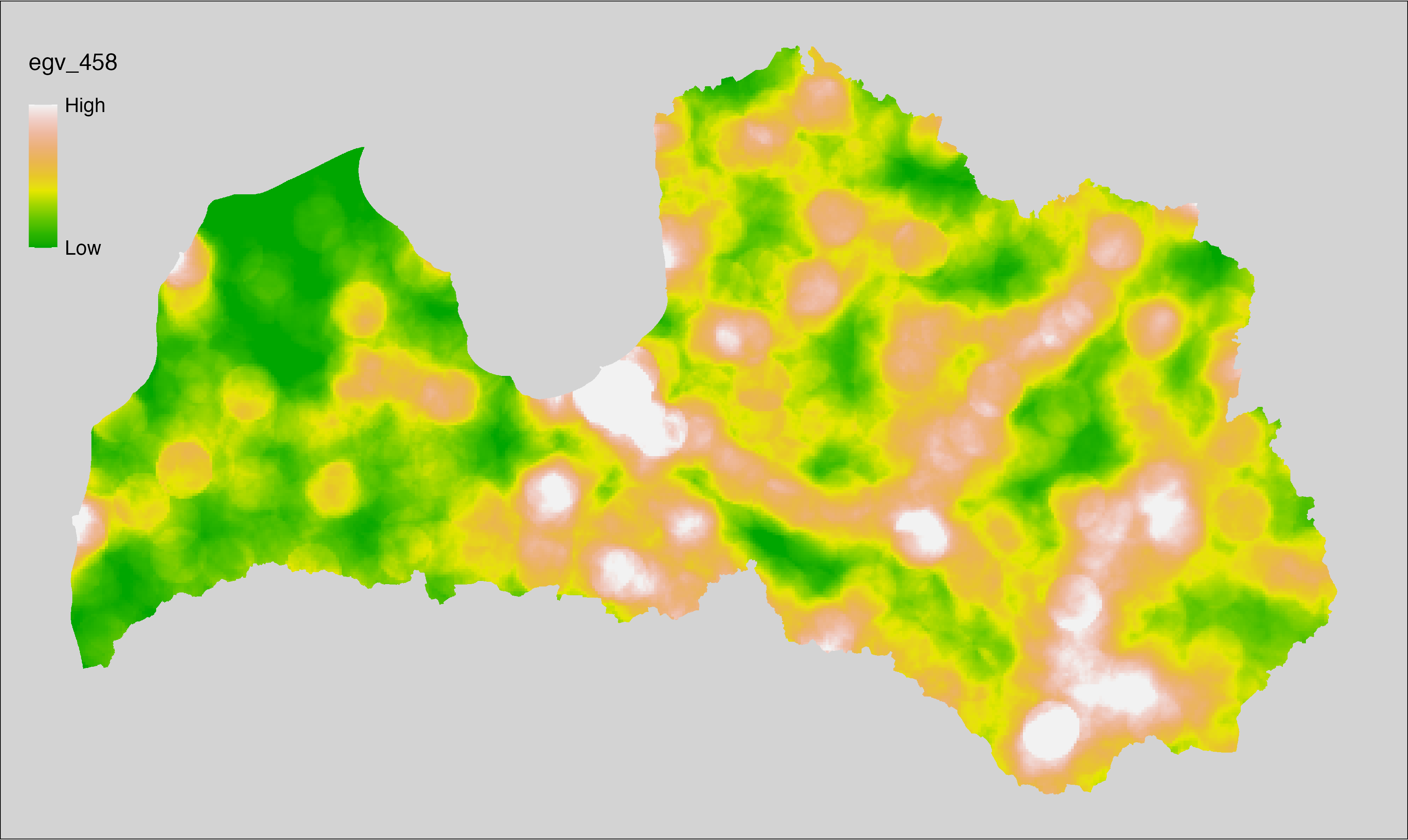
6.459 General_Water_cell
filename: General_Water_cell.tif
layername: egv_459
English name: Fractional cover of Waterbodies within the analysis cell (1 ha)
Latvian name: Ūdenstilpju platības īpatsvars analīzes šūnā (1 ha)
Procedure: First, the waters from the Landscape classification are
selected (value 200 is reclassified to value 1; all others are set to 0). The resulting layer
is then aggregated to EGV resolution using the workflow egvtools::input2egv(), which
calculates the arithmetic mean to determine the cover fraction. During
aggregation, inverse distance weighted (power = 2) gap filling on the output is
applied to ensure no missing values at the edges. Finally, the layer is
standardised by subtracting the arithmetic mean and dividing by the root mean squared
error.
Code
# libs ----
if(!require(egvtools)) {remotes::install_github("aavotins/egvtools"); require(egvtools)}
if(!require(terra)) {install.packages("terra"); require(terra)}
if(!require(sf)) {install.packages("sf"); require(sf)}
if(!require(tidyverse)) {install.packages("tidyverse"); require(tidyverse)}
if(!require(sfarrow)) {install.packages("sfarrow"); require(sfarrow)}
if(!require(readxl)) {install.packages("readxl"); require(readxl)}
if(!require(raster)) {install.packages("raster"); require(raster)}
if(!require(fasterize)) {install.packages("fasterize"); require(fasterize)}
# templates ----
template100=rast("./Templates/TemplateRasters/LV100m_10km.tif")
template10=rast("./Templates/TemplateRasters/LV10m_10km.tif")
rastrs10=raster(template10)
nulls10=rast("./Templates/TemplateRasters/nulls_LV10m_10km.tif")
nulls100=rast("./Templates/TemplateRasters/nulls_LV100m_10km.tif")
# simple landscape ----
simple_landscape=rast("RasterGrids_10m/2024/Ainava_vienk_mask.tif")
# General_Water_cell.tif egv_459 ----
udens=ifel(simple_landscape==200,1,0)
i2e_rez=egvtools::input2egv(input=udens,
egv_template= "./Templates/TemplateRasters/LV100m_10km.tif",
summary_function = "average",
missing_job = "FillOutput",
outlocation = "./RasterGrids_100m/2024/RAW/",
outfilename = "General_Water_cell.tif",
layername = "egv_459",
idw_weight = 2,
plot_gaps = FALSE,plot_final = TRUE)
i2e_rez
rm(udens)
rm(i2e_rez)
# standardisation ----
if(!require(terra)) {install.packages("terra"); require(terra)}
if(!require(tidyverse)) {install.packages("tidyverse"); require(tidyverse)}
nosaukums="General_Water_cell.tif"
ielasisanas_cels=paste0("./RasterGrids_100m/2024/RAW/",nosaukums)
saglabasanas_cels=paste0("./RasterGrids_100m/2024/Scaled/",nosaukums)
slanis=rast(ielasisanas_cels)
videjais=global(slanis,fun="mean",na.rm=TRUE)
centrets=slanis-videjais[,1]
standartnovirze=terra::global(centrets,fun="rms",na.rm=TRUE)
merogots=centrets/standartnovirze[,1]
writeRaster(merogots,
filename=saglabasanas_cels,
overwrite=TRUE)
6.460 General_Water_r500
filename: General_Water_r500.tif
layername: egv_460
English name: Fractional cover of Waterbodies within the 0.5 km landscape
Latvian name: Ūdenstilpju platības īpatsvars 0,5 km ainavā
Procedure: The cover fraction within a radius of 500 m around the analysis grid cell is
calculated as the area-weighted sum of the analysis cells inside the
buffer, using the workflow egvtools::radius_function(). During the calculation of the landscape metric,
inverse distance weighted (power = 2) gap filling on the output is applied
to ensure no missing values at the edges. Then the layer is rewritten to set
its name. Finally, the layer is standardised by subtracting the arithmetic
mean and dividing by the root mean squared error.
Code
# libs ----
if(!require(terra)) {install.packages("terra"); require(terra)}
if(!require(egvtools)) {remotes::install_github("aavotins/egvtools"); require(egvtools)}
# Templates -----
template100=rast("./Templates/TemplateRasters/LV100m_10km.tif")
# radii ----
radius_function(
kvadrati_path = "./Templates/TemplateGrids/tiles/",
radii_path = "./Templates/TemplateGridPoints/tiles/",
tikls100_path = "./Templates/TemplateGrids/tikls100_sauzeme.parquet",
template_path = "./Templates/TemplateRasters/LV100m_10km.tif",
input_layers = c("./RasterGrids_100m/2024/RAW/General_Water_cell.tif"),
layer_prefixes = c("General_Water"),
output_dir = "./RasterGrids_100m/2024/RAW/",
n_workers = 6,
radii = c("r500"),
radius_mode = "sparse",
extract_fun = "mean",
fill_missing = TRUE,
IDW_weight = 2,
future_max_size = 40 * 1024^3)
# General_Water_r500.tif egv_460
slanis=rast("./RasterGrids_100m/2024/RAW/General_Water_r500.tif")
names(slanis)="egv_460"
slanis2=project(slanis,template100)
writeRaster(slanis2,
"./RasterGrids_100m/2024/RAW/General_Water_r500.tif",
overwrite=TRUE)
# standardisation ----
if(!require(terra)) {install.packages("terra"); require(terra)}
if(!require(tidyverse)) {install.packages("tidyverse"); require(tidyverse)}
nosaukums="General_Water_r500.tif"
ielasisanas_cels=paste0("./RasterGrids_100m/2024/RAW/",nosaukums)
saglabasanas_cels=paste0("./RasterGrids_100m/2024/Scaled/",nosaukums)
slanis=rast(ielasisanas_cels)
videjais=global(slanis,fun="mean",na.rm=TRUE)
centrets=slanis-videjais[,1]
standartnovirze=terra::global(centrets,fun="rms",na.rm=TRUE)
merogots=centrets/standartnovirze[,1]
writeRaster(merogots,
filename=saglabasanas_cels,
overwrite=TRUE)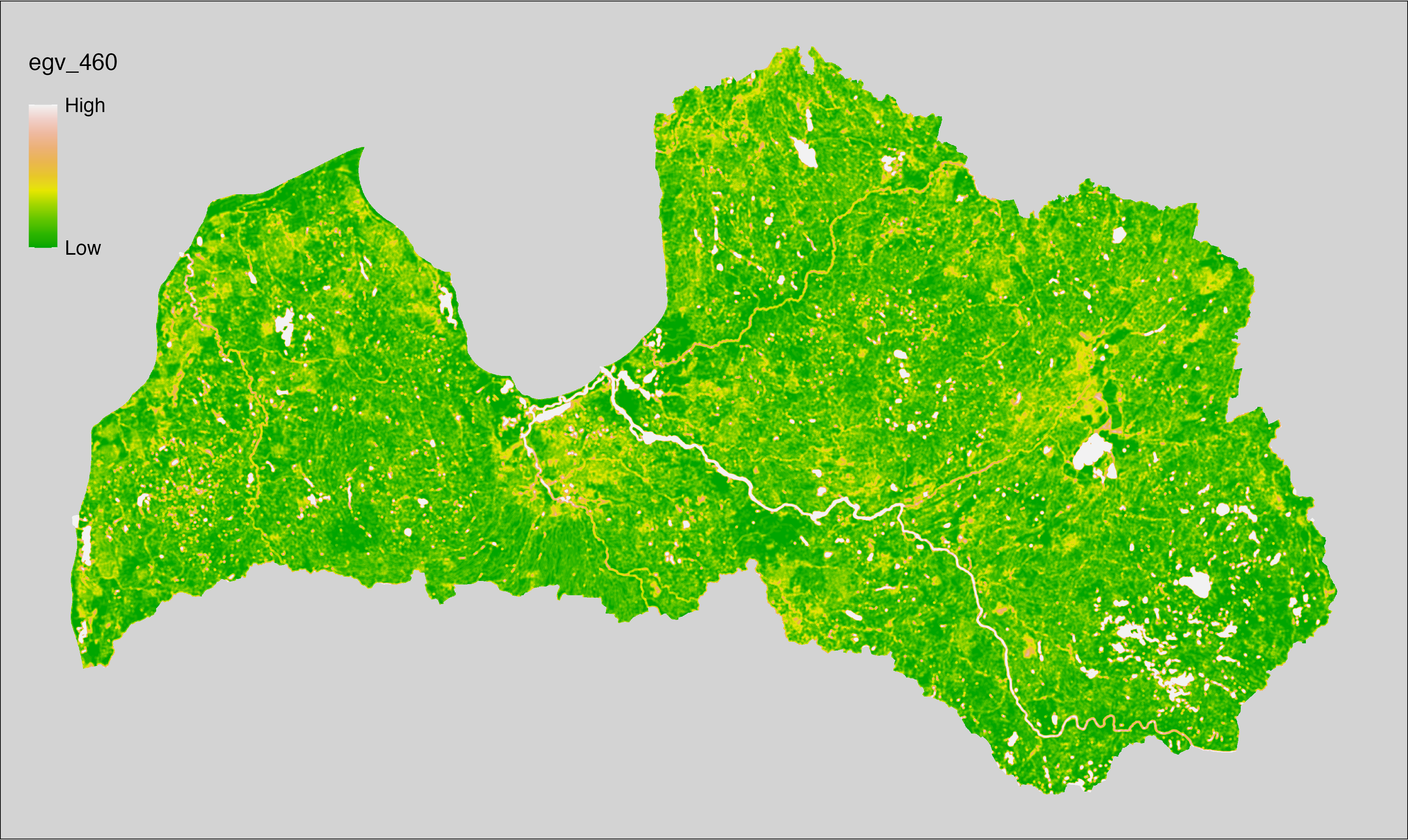
6.461 General_Water_r1250
filename: General_Water_r1250.tif
layername: egv_461
English name: Fractional cover of Waterbodies within the 1.25 km landscape
Latvian name: Ūdenstilpju platības īpatsvars 1,25 km ainavā
Procedure: The cover fraction within a radius of 1250 m around the analysis grid cell
is calculated as the area-weighted sum of the analysis cells inside
the buffer, using the workflow egvtools::radius_function(). During the calculation of the landscape
metric, inverse distance weighted (power = 2) gap filling on the output is
applied to ensure no missing values at the edges. Then the layer is
rewritten to set its name. Finally, the layer is standardised by
subtracting the arithmetic mean and dividing by the root mean squared error.
Code
# libs ----
if(!require(terra)) {install.packages("terra"); require(terra)}
if(!require(egvtools)) {remotes::install_github("aavotins/egvtools"); require(egvtools)}
# Templates -----
template100=rast("./Templates/TemplateRasters/LV100m_10km.tif")
# radii ----
radius_function(
kvadrati_path = "./Templates/TemplateGrids/tiles/",
radii_path = "./Templates/TemplateGridPoints/tiles/",
tikls100_path = "./Templates/TemplateGrids/tikls100_sauzeme.parquet",
template_path = "./Templates/TemplateRasters/LV100m_10km.tif",
input_layers = c("./RasterGrids_100m/2024/RAW/General_Water_cell.tif"),
layer_prefixes = c("General_Water"),
output_dir = "./RasterGrids_100m/2024/RAW/",
n_workers = 6,
radii = c("r1250"),
radius_mode = "sparse",
extract_fun = "mean",
fill_missing = TRUE,
IDW_weight = 2,
future_max_size = 40 * 1024^3)
# General_Water_r1250.tif egv_461
slanis=rast("./RasterGrids_100m/2024/RAW/General_Water_r1250.tif")
names(slanis)="egv_461"
slanis2=project(slanis,template100)
writeRaster(slanis2,
"./RasterGrids_100m/2024/RAW/General_Water_r1250.tif",
overwrite=TRUE)
# standardisation ----
if(!require(terra)) {install.packages("terra"); require(terra)}
if(!require(tidyverse)) {install.packages("tidyverse"); require(tidyverse)}
nosaukums="General_Water_r1250.tif"
ielasisanas_cels=paste0("./RasterGrids_100m/2024/RAW/",nosaukums)
saglabasanas_cels=paste0("./RasterGrids_100m/2024/Scaled/",nosaukums)
slanis=rast(ielasisanas_cels)
videjais=global(slanis,fun="mean",na.rm=TRUE)
centrets=slanis-videjais[,1]
standartnovirze=terra::global(centrets,fun="rms",na.rm=TRUE)
merogots=centrets/standartnovirze[,1]
writeRaster(merogots,
filename=saglabasanas_cels,
overwrite=TRUE)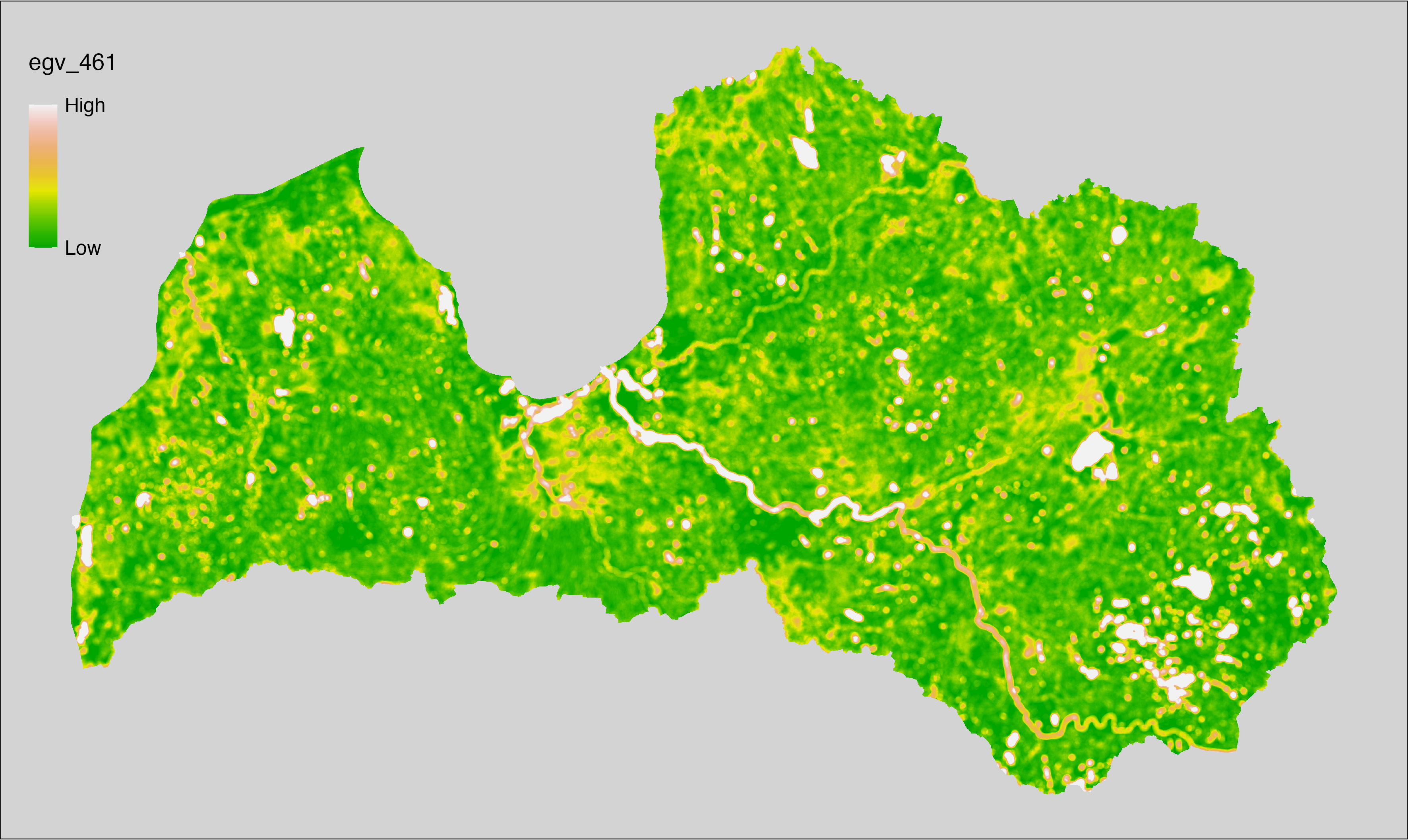
6.462 General_Water_r3000
filename: General_Water_r3000.tif
layername: egv_462
English name: Fractional cover of Waterbodies within the 3 km landscape
Latvian name: Ūdenstilpju platības īpatsvars 3 km ainavā
Procedure: The cover fraction within a radius of 3000 m around the analysis grid cell
is calculated as the area-weighted sum of the analysis cells inside
the buffer, using the workflow egvtools::radius_function(). During the calculation of the landscape
metric, inverse distance weighted (power = 2) gap filling on the output is
applied to ensure no missing values at the edges. Then the layer is
rewritten to set its name. Finally, the layer is standardised by
subtracting the arithmetic mean and dividing by the root mean squared error.
Code
# libs ----
if(!require(terra)) {install.packages("terra"); require(terra)}
if(!require(egvtools)) {remotes::install_github("aavotins/egvtools"); require(egvtools)}
# Templates -----
template100=rast("./Templates/TemplateRasters/LV100m_10km.tif")
# radii ----
radius_function(
kvadrati_path = "./Templates/TemplateGrids/tiles/",
radii_path = "./Templates/TemplateGridPoints/tiles/",
tikls100_path = "./Templates/TemplateGrids/tikls100_sauzeme.parquet",
template_path = "./Templates/TemplateRasters/LV100m_10km.tif",
input_layers = c("./RasterGrids_100m/2024/RAW/General_Water_cell.tif"),
layer_prefixes = c("General_Water"),
output_dir = "./RasterGrids_100m/2024/RAW/",
n_workers = 6,
radii = c("r3000"),
radius_mode = "sparse",
extract_fun = "mean",
fill_missing = TRUE,
IDW_weight = 2,
future_max_size = 40 * 1024^3)
# General_Water_r3000.tif egv_462
slanis=rast("./RasterGrids_100m/2024/RAW/General_Water_r3000.tif")
names(slanis)="egv_462"
slanis2=project(slanis,template100)
writeRaster(slanis2,
"./RasterGrids_100m/2024/RAW/General_Water_r3000.tif",
overwrite=TRUE)
# standardisation ----
if(!require(terra)) {install.packages("terra"); require(terra)}
if(!require(tidyverse)) {install.packages("tidyverse"); require(tidyverse)}
nosaukums="General_Water_r3000.tif"
ielasisanas_cels=paste0("./RasterGrids_100m/2024/RAW/",nosaukums)
saglabasanas_cels=paste0("./RasterGrids_100m/2024/Scaled/",nosaukums)
slanis=rast(ielasisanas_cels)
videjais=global(slanis,fun="mean",na.rm=TRUE)
centrets=slanis-videjais[,1]
standartnovirze=terra::global(centrets,fun="rms",na.rm=TRUE)
merogots=centrets/standartnovirze[,1]
writeRaster(merogots,
filename=saglabasanas_cels,
overwrite=TRUE)
6.463 General_Water_r10000
filename: General_Water_r10000.tif
layername: egv_463
English name: Fractional cover of Waterbodies within the 10 km landscape
Latvian name: Ūdenstilpju platības īpatsvars 10 km ainavā
Procedure: The cover fraction within a radius of 10000 m around the analysis grid cell
is calculated as the area-weighted sum of the analysis cells inside
the buffer, using the workflow egvtools::radius_function(). During the calculation of the landscape
metric, inverse distance weighted (power = 2) gap filling on the output is
applied to ensure no missing values at the edges. Then the layer is
rewritten to set its name. Finally, the layer is standardised by
subtracting the arithmetic mean and dividing by the root mean squared error.
Code
# libs ----
if(!require(terra)) {install.packages("terra"); require(terra)}
if(!require(egvtools)) {remotes::install_github("aavotins/egvtools"); require(egvtools)}
# Templates -----
template100=rast("./Templates/TemplateRasters/LV100m_10km.tif")
# radii ----
radius_function(
kvadrati_path = "./Templates/TemplateGrids/tiles/",
radii_path = "./Templates/TemplateGridPoints/tiles/",
tikls100_path = "./Templates/TemplateGrids/tikls100_sauzeme.parquet",
template_path = "./Templates/TemplateRasters/LV100m_10km.tif",
input_layers = c("./RasterGrids_100m/2024/RAW/General_Water_cell.tif"),
layer_prefixes = c("General_Water"),
output_dir = "./RasterGrids_100m/2024/RAW/",
n_workers = 6,
radii = c("r10000"),
radius_mode = "sparse",
extract_fun = "mean",
fill_missing = TRUE,
IDW_weight = 2,
future_max_size = 40 * 1024^3)
# General_Water_r10000.tif egv_463
slanis=rast("./RasterGrids_100m/2024/RAW/General_Water_r10000.tif")
names(slanis)="egv_463"
slanis2=project(slanis,template100)
writeRaster(slanis2,
"./RasterGrids_100m/2024/RAW/General_Water_r10000.tif",
overwrite=TRUE)
# standardisation ----
if(!require(terra)) {install.packages("terra"); require(terra)}
if(!require(tidyverse)) {install.packages("tidyverse"); require(tidyverse)}
nosaukums="General_Water_r10000.tif"
ielasisanas_cels=paste0("./RasterGrids_100m/2024/RAW/",nosaukums)
saglabasanas_cels=paste0("./RasterGrids_100m/2024/Scaled/",nosaukums)
slanis=rast(ielasisanas_cels)
videjais=global(slanis,fun="mean",na.rm=TRUE)
centrets=slanis-videjais[,1]
standartnovirze=terra::global(centrets,fun="rms",na.rm=TRUE)
merogots=centrets/standartnovirze[,1]
writeRaster(merogots,
filename=saglabasanas_cels,
overwrite=TRUE)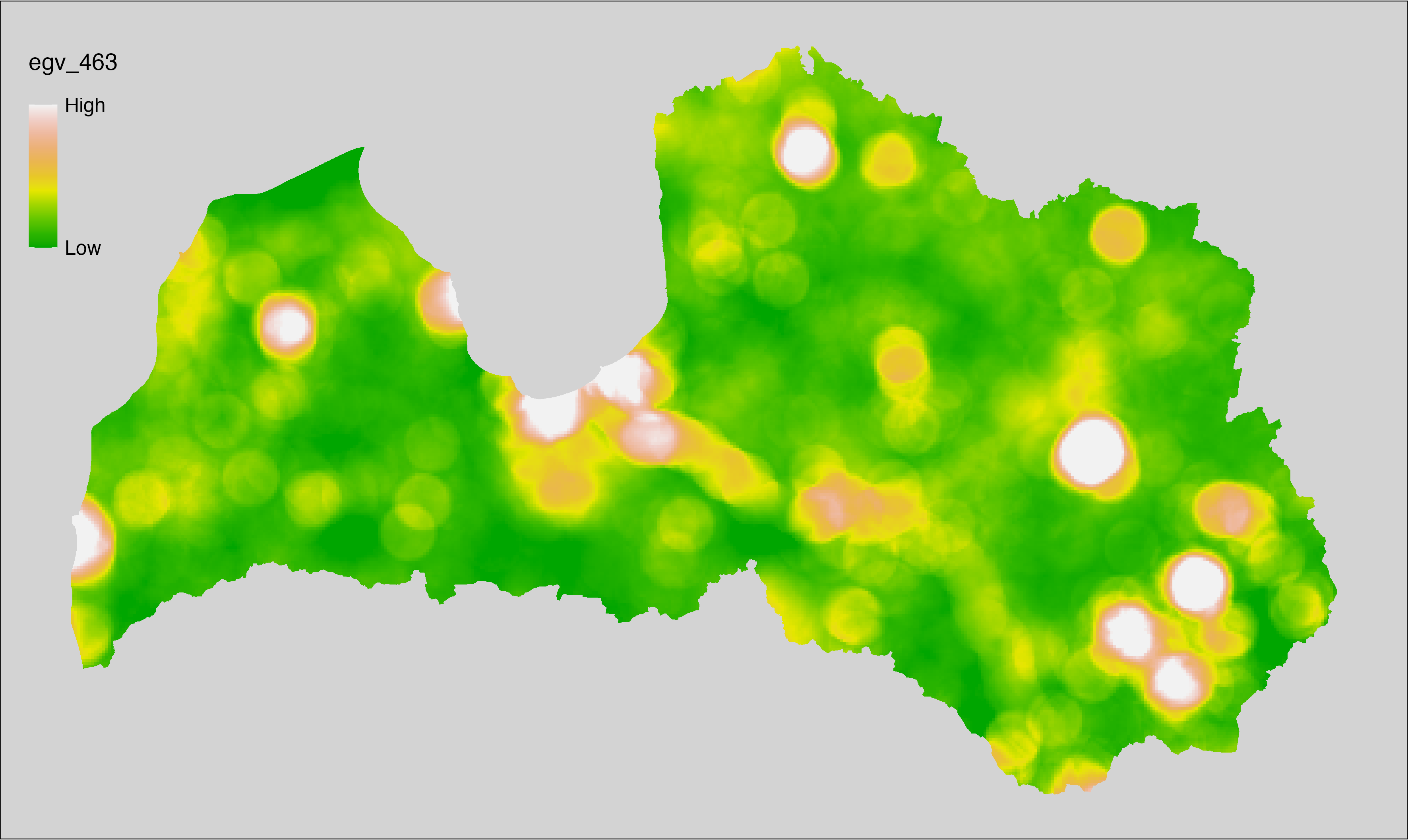
6.464 Wetlands_Bogs_cell
filename: Wetlands_Bogs_cell.tif
layername: egv_464
English name: Fractional cover of Raised Bogs within the analysis cell (1 ha)
Latvian name: Augsto purvu platības īpatsvars analīzes šūnā (1 ha)
Procedure: Derived from the Bogs and Mires: EDI, where bogs are
classified as 1 with 0 elsewhere. The resulting layer
is then aggregated to EGV resolution using the workflow egvtools::input2egv(), which
calculates the arithmetic mean to determine the cover fraction. During
aggregation, inverse distance weighted (power = 2) gap filling on the output is
applied to ensure no missing values at the edges. Finally, the layer is
standardised by subtracting the arithmetic mean and dividing by the root mean squared
error.
Code
# libs ----
if(!require(egvtools)) {remotes::install_github("aavotins/egvtools"); require(egvtools)}
if(!require(terra)) {install.packages("terra"); require(terra)}
# template ----
template100=rast("./Templates/TemplateRasters/LV100m_10km.tif")
# Wetlands_Bogs_cell.tif egv_464 ----
bogs=rast("./RasterGrids_10m/2024/EDI_BogsYN.tif")
i2e_rez=egvtools::input2egv(input=bogs,
egv_template= "./Templates/TemplateRasters/LV100m_10km.tif",
summary_function = "average",
missing_job = "FillOutput",
outlocation = "./RasterGrids_100m/2024/RAW/",
outfilename = "Wetlands_Bogs_cell.tif",
layername = "egv_464",
idw_weight = 2,
plot_gaps = FALSE,plot_final = TRUE)
i2e_rez
rm(bogs)
rm(i2e_rez)
# standardisation ----
if(!require(terra)) {install.packages("terra"); require(terra)}
if(!require(tidyverse)) {install.packages("tidyverse"); require(tidyverse)}
nosaukums="Wetlands_Bogs_cell.tif"
ielasisanas_cels=paste0("./RasterGrids_100m/2024/RAW/",nosaukums)
saglabasanas_cels=paste0("./RasterGrids_100m/2024/Scaled/",nosaukums)
slanis=rast(ielasisanas_cels)
videjais=global(slanis,fun="mean",na.rm=TRUE)
centrets=slanis-videjais[,1]
standartnovirze=terra::global(centrets,fun="rms",na.rm=TRUE)
merogots=centrets/standartnovirze[,1]
writeRaster(merogots,
filename=saglabasanas_cels,
overwrite=TRUE)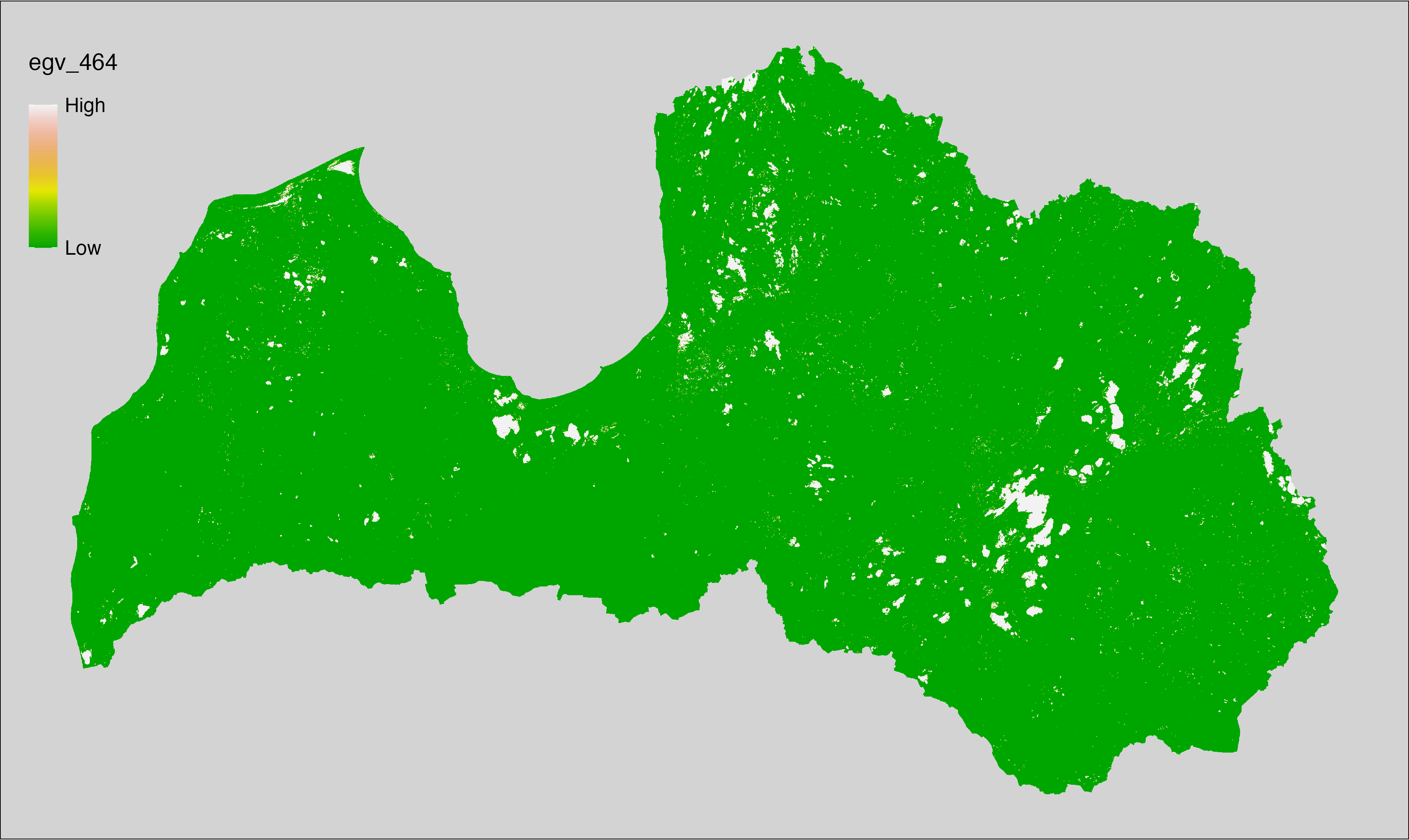
6.465 Wetlands_Bogs_r500
filename: Wetlands_Bogs_r500.tif
layername: egv_465
English name: Fractional cover of Raised Bogs within the 0.5 km landscape
Latvian name: Augsto purvu platības īpatsvars 0,5 km ainavā
Procedure: The cover fraction within a radius of 500 m around the analysis grid cell is
calculated as the area-weighted sum of the analysis cells inside the
buffer, using the workflow egvtools::radius_function(). During the calculation of the landscape metric,
inverse distance weighted (power = 2) gap filling on the output is applied
to ensure no missing values at the edges. Then the layer is rewritten to set
its name. Finally, the layer is standardised by subtracting the arithmetic
mean and dividing by the root mean squared error.
Code
# libs ----
if(!require(terra)) {install.packages("terra"); require(terra)}
if(!require(egvtools)) {remotes::install_github("aavotins/egvtools"); require(egvtools)}
# Templates -----
template100=rast("./Templates/TemplateRasters/LV100m_10km.tif")
# radii ----
radius_function(
kvadrati_path = "./Templates/TemplateGrids/tiles/",
radii_path = "./Templates/TemplateGridPoints/tiles/",
tikls100_path = "./Templates/TemplateGrids/tikls100_sauzeme.parquet",
template_path = "./Templates/TemplateRasters/LV100m_10km.tif",
input_layers = c("./RasterGrids_100m/2024/RAW/Wetlands_Bogs_cell.tif"),
layer_prefixes = c("Wetlands_Bogs"),
output_dir = "./RasterGrids_100m/2024/RAW/",
n_workers = 12,
radii = c("r500"),
radius_mode = "sparse",
extract_fun = "mean",
fill_missing = TRUE,
IDW_weight = 2,
future_max_size = 20 * 1024^3)
# Wetlands_Bogs_r500.tif egv_465
slanis=rast("./RasterGrids_100m/2024/RAW/Wetlands_Bogs_r500.tif")
names(slanis)="egv_465"
slanis2=project(slanis,template100)
writeRaster(slanis2,
"./RasterGrids_100m/2024/RAW/Wetlands_Bogs_r500.tif",
overwrite=TRUE)
# standardisation ----
if(!require(terra)) {install.packages("terra"); require(terra)}
if(!require(tidyverse)) {install.packages("tidyverse"); require(tidyverse)}
nosaukums="Wetlands_Bogs_r500.tif"
ielasisanas_cels=paste0("./RasterGrids_100m/2024/RAW/",nosaukums)
saglabasanas_cels=paste0("./RasterGrids_100m/2024/Scaled/",nosaukums)
slanis=rast(ielasisanas_cels)
videjais=global(slanis,fun="mean",na.rm=TRUE)
centrets=slanis-videjais[,1]
standartnovirze=terra::global(centrets,fun="rms",na.rm=TRUE)
merogots=centrets/standartnovirze[,1]
writeRaster(merogots,
filename=saglabasanas_cels,
overwrite=TRUE)
6.466 Wetlands_Bogs_r1250
filename: Wetlands_Bogs_r1250.tif
layername: egv_466
English name: Fractional cover of Raised Bogs within the 1.25 km landscape
Latvian name: Augsto purvu platības īpatsvars 1,25 km ainavā
Procedure: The cover fraction within a radius of 1250 m around the analysis grid cell
is calculated as the area-weighted sum of the analysis cells inside
the buffer, using the workflow egvtools::radius_function(). During the calculation of the landscape
metric, inverse distance weighted (power = 2) gap filling on the output is
applied to ensure no missing values at the edges. Then the layer is
rewritten to set its name. Finally, the layer is standardised by
subtracting the arithmetic mean and dividing by the root mean squared error.
Code
# libs ----
if(!require(terra)) {install.packages("terra"); require(terra)}
if(!require(egvtools)) {remotes::install_github("aavotins/egvtools"); require(egvtools)}
# Templates -----
template100=rast("./Templates/TemplateRasters/LV100m_10km.tif")
# radii ----
radius_function(
kvadrati_path = "./Templates/TemplateGrids/tiles/",
radii_path = "./Templates/TemplateGridPoints/tiles/",
tikls100_path = "./Templates/TemplateGrids/tikls100_sauzeme.parquet",
template_path = "./Templates/TemplateRasters/LV100m_10km.tif",
input_layers = c("./RasterGrids_100m/2024/RAW/Wetlands_Bogs_cell.tif"),
layer_prefixes = c("Wetlands_Bogs"),
output_dir = "./RasterGrids_100m/2024/RAW/",
n_workers = 12,
radii = c("r1250"),
radius_mode = "sparse",
extract_fun = "mean",
fill_missing = TRUE,
IDW_weight = 2,
future_max_size = 20 * 1024^3)
# Wetlands_Bogs_r1250.tif egv_466
slanis=rast("./RasterGrids_100m/2024/RAW/Wetlands_Bogs_r1250.tif")
names(slanis)="egv_466"
slanis2=project(slanis,template100)
writeRaster(slanis2,
"./RasterGrids_100m/2024/RAW/Wetlands_Bogs_r1250.tif",
overwrite=TRUE)
# standardisation ----
if(!require(terra)) {install.packages("terra"); require(terra)}
if(!require(tidyverse)) {install.packages("tidyverse"); require(tidyverse)}
nosaukums="Wetlands_Bogs_r1250.tif"
ielasisanas_cels=paste0("./RasterGrids_100m/2024/RAW/",nosaukums)
saglabasanas_cels=paste0("./RasterGrids_100m/2024/Scaled/",nosaukums)
slanis=rast(ielasisanas_cels)
videjais=global(slanis,fun="mean",na.rm=TRUE)
centrets=slanis-videjais[,1]
standartnovirze=terra::global(centrets,fun="rms",na.rm=TRUE)
merogots=centrets/standartnovirze[,1]
writeRaster(merogots,
filename=saglabasanas_cels,
overwrite=TRUE)
6.467 Wetlands_Bogs_r3000
filename: Wetlands_Bogs_r3000.tif
layername: egv_467
English name: Fractional cover of Raised Bogs within the 3 km landscape
Latvian name: Augsto purvu platības īpatsvars 3 km ainavā
Procedure: The cover fraction within a radius of 3000 m around the analysis grid cell
is calculated as the area-weighted sum of the analysis cells inside
the buffer, using the workflow egvtools::radius_function(). During the calculation of the landscape
metric, inverse distance weighted (power = 2) gap filling on the output is
applied to ensure no missing values at the edges. Then the layer is
rewritten to set its name. Finally, the layer is standardised by
subtracting the arithmetic mean and dividing by the root mean squared error.
Code
# libs ----
if(!require(terra)) {install.packages("terra"); require(terra)}
if(!require(egvtools)) {remotes::install_github("aavotins/egvtools"); require(egvtools)}
# Templates -----
template100=rast("./Templates/TemplateRasters/LV100m_10km.tif")
# radii ----
radius_function(
kvadrati_path = "./Templates/TemplateGrids/tiles/",
radii_path = "./Templates/TemplateGridPoints/tiles/",
tikls100_path = "./Templates/TemplateGrids/tikls100_sauzeme.parquet",
template_path = "./Templates/TemplateRasters/LV100m_10km.tif",
input_layers = c("./RasterGrids_100m/2024/RAW/Wetlands_Bogs_cell.tif"),
layer_prefixes = c("Wetlands_Bogs"),
output_dir = "./RasterGrids_100m/2024/RAW/",
n_workers = 12,
radii = c("r3000"),
radius_mode = "sparse",
extract_fun = "mean",
fill_missing = TRUE,
IDW_weight = 2,
future_max_size = 20 * 1024^3)
# Wetlands_Bogs_r3000.tif egv_467
slanis=rast("./RasterGrids_100m/2024/RAW/Wetlands_Bogs_r3000.tif")
names(slanis)="egv_467"
slanis2=project(slanis,template100)
writeRaster(slanis2,
"./RasterGrids_100m/2024/RAW/Wetlands_Bogs_r3000.tif",
overwrite=TRUE)
# standardisation ----
if(!require(terra)) {install.packages("terra"); require(terra)}
if(!require(tidyverse)) {install.packages("tidyverse"); require(tidyverse)}
nosaukums="Wetlands_Bogs_r3000.tif"
ielasisanas_cels=paste0("./RasterGrids_100m/2024/RAW/",nosaukums)
saglabasanas_cels=paste0("./RasterGrids_100m/2024/Scaled/",nosaukums)
slanis=rast(ielasisanas_cels)
videjais=global(slanis,fun="mean",na.rm=TRUE)
centrets=slanis-videjais[,1]
standartnovirze=terra::global(centrets,fun="rms",na.rm=TRUE)
merogots=centrets/standartnovirze[,1]
writeRaster(merogots,
filename=saglabasanas_cels,
overwrite=TRUE)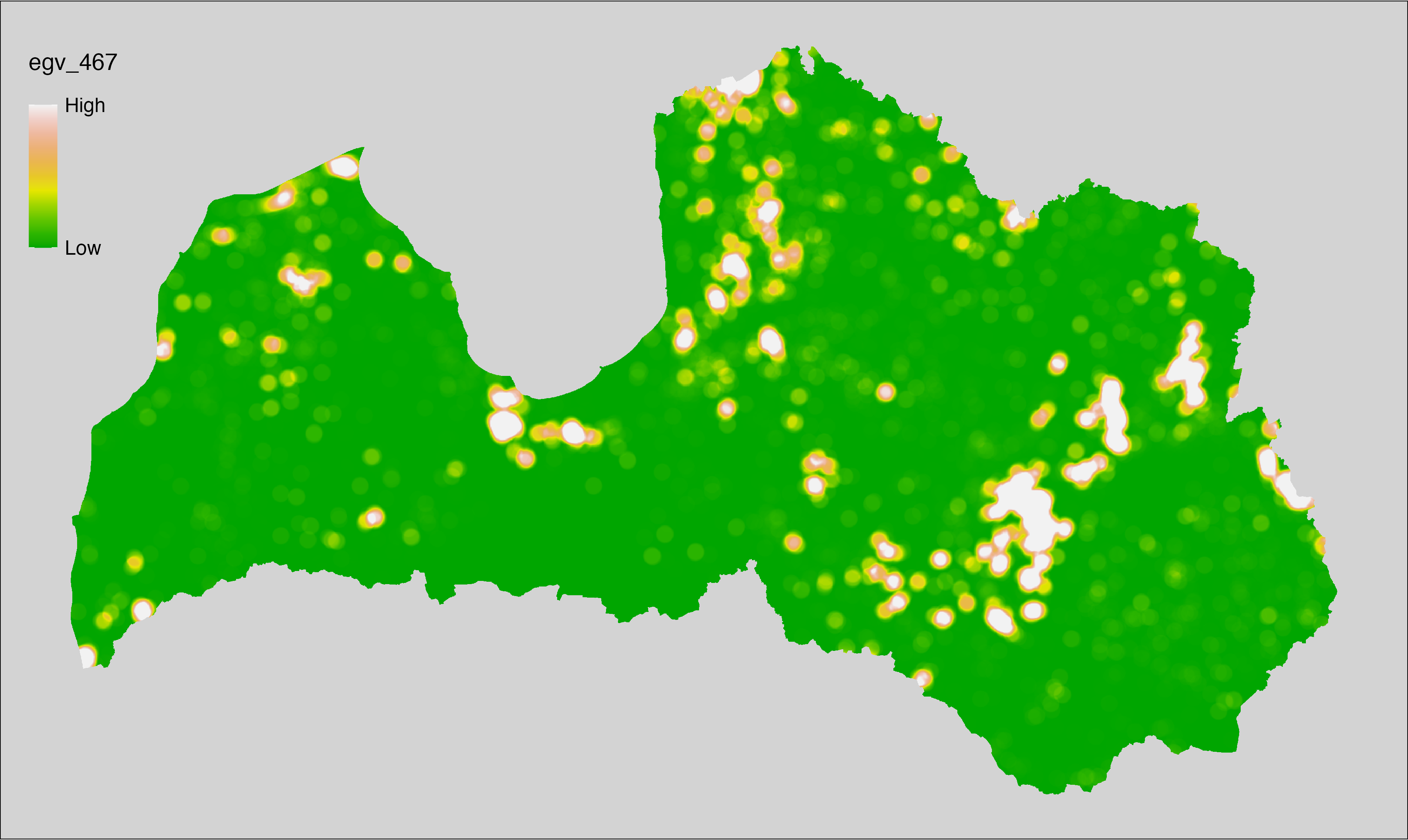
6.468 Wetlands_Bogs_r10000
filename: Wetlands_Bogs_r10000.tif
layername: egv_468
English name: Fractional cover of Raised Bogs within the 10 km landscape
Latvian name: Augsto purvu platības īpatsvars 10 km ainavā
Procedure: The cover fraction within a radius of 10000 m around the analysis grid cell
is calculated as the area-weighted sum of the analysis cells inside
the buffer, using the workflow egvtools::radius_function(). During the calculation of the landscape
metric, inverse distance weighted (power = 2) gap filling on the output is
applied to ensure no missing values at the edges. Then the layer is
rewritten to set its name. Finally, the layer is standardised by
subtracting the arithmetic mean and dividing by the root mean squared error.
Code
# libs ----
if(!require(terra)) {install.packages("terra"); require(terra)}
if(!require(egvtools)) {remotes::install_github("aavotins/egvtools"); require(egvtools)}
# Templates -----
template100=rast("./Templates/TemplateRasters/LV100m_10km.tif")
# radii ----
radius_function(
kvadrati_path = "./Templates/TemplateGrids/tiles/",
radii_path = "./Templates/TemplateGridPoints/tiles/",
tikls100_path = "./Templates/TemplateGrids/tikls100_sauzeme.parquet",
template_path = "./Templates/TemplateRasters/LV100m_10km.tif",
input_layers = c("./RasterGrids_100m/2024/RAW/Wetlands_Bogs_cell.tif"),
layer_prefixes = c("Wetlands_Bogs"),
output_dir = "./RasterGrids_100m/2024/RAW/",
n_workers = 12,
radii = c("r10000"),
radius_mode = "sparse",
extract_fun = "mean",
fill_missing = TRUE,
IDW_weight = 2,
future_max_size = 20 * 1024^3)
# Wetlands_Bogs_r10000.tif egv_468
slanis=rast("./RasterGrids_100m/2024/RAW/Wetlands_Bogs_r10000.tif")
names(slanis)="egv_468"
slanis2=project(slanis,template100)
writeRaster(slanis2,
"./RasterGrids_100m/2024/RAW/Wetlands_Bogs_r10000.tif",
overwrite=TRUE)
# standardisation ----
if(!require(terra)) {install.packages("terra"); require(terra)}
if(!require(tidyverse)) {install.packages("tidyverse"); require(tidyverse)}
nosaukums="Wetlands_Bogs_r10000.tif"
ielasisanas_cels=paste0("./RasterGrids_100m/2024/RAW/",nosaukums)
saglabasanas_cels=paste0("./RasterGrids_100m/2024/Scaled/",nosaukums)
slanis=rast(ielasisanas_cels)
videjais=global(slanis,fun="mean",na.rm=TRUE)
centrets=slanis-videjais[,1]
standartnovirze=terra::global(centrets,fun="rms",na.rm=TRUE)
merogots=centrets/standartnovirze[,1]
writeRaster(merogots,
filename=saglabasanas_cels,
overwrite=TRUE)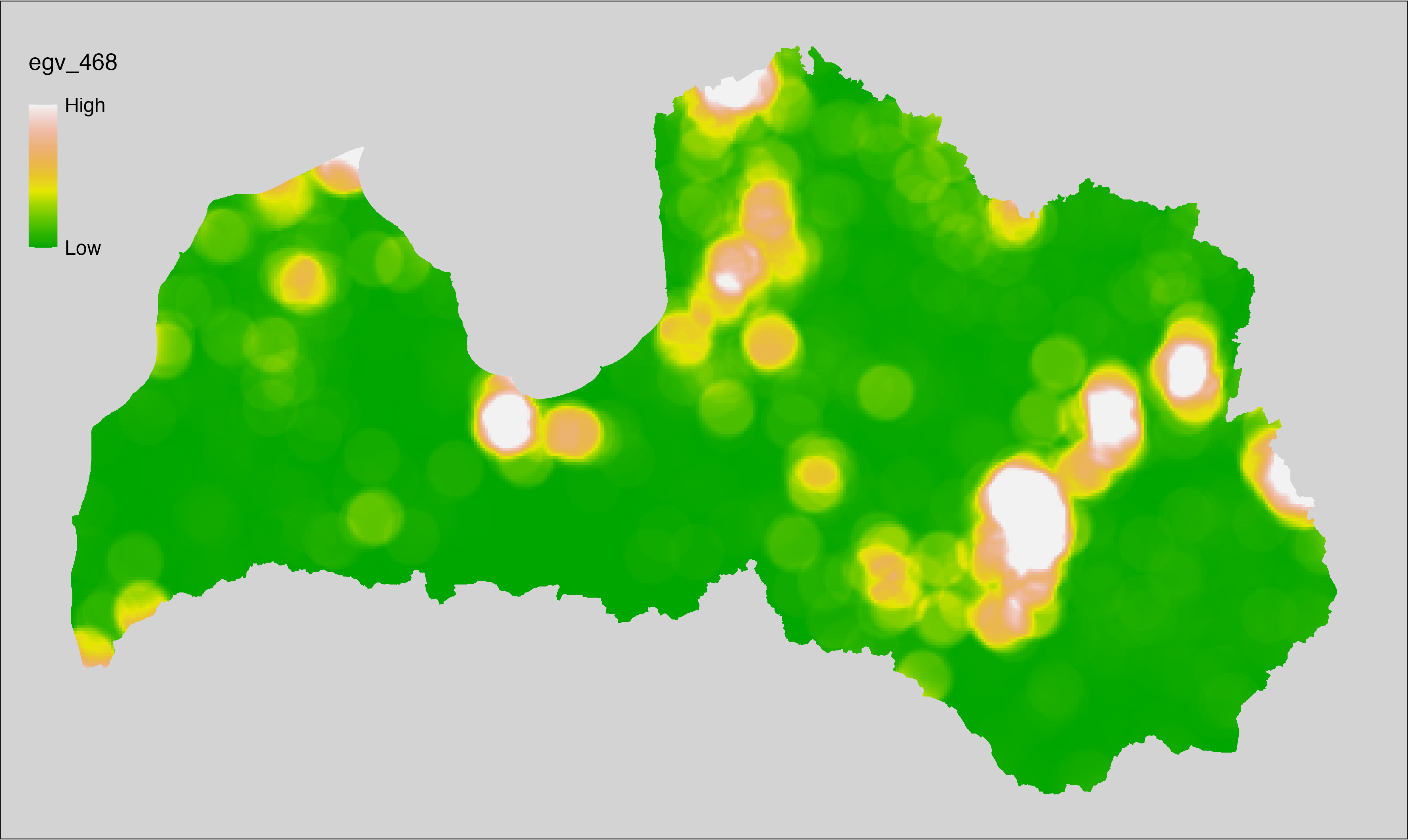
6.469 Wetlands_Mires_cell
filename: Wetlands_Mires_cell.tif
layername: egv_469
English name: Fractional cover of Transitional Mires within the analysis cell (1 ha)
Latvian name: Pārejas purvu platības īpatsvars analīzes šūnā (1 ha)
Procedure: Derived from the Bogs and Mires: EDI, where transitional
mires are classified as 1 with 0 elsewhere. The resulting layer
is then aggregated to EGV resolution using the workflow egvtools::input2egv(), which
calculates the arithmetic mean to determine the cover fraction. During
aggregation, inverse distance weighted (power = 2) gap filling on the output is
applied to ensure no missing values at the edges. Finally, the layer is
standardised by subtracting the arithmetic mean and dividing by the root mean squared
error.
Code
# libs ----
if(!require(egvtools)) {remotes::install_github("aavotins/egvtools"); require(egvtools)}
if(!require(terra)) {install.packages("terra"); require(terra)}
# template ----
template100=rast("./Templates/TemplateRasters/LV100m_10km.tif")
# Wetlands_Mires_cell.tif egv_469 ----
mires=rast("./RasterGrids_10m/2024/EDI_TransitionalMiresYN.tif")
i2e_rez=egvtools::input2egv(input=mires,
egv_template= "./Templates/TemplateRasters/LV100m_10km.tif",
summary_function = "average",
missing_job = "FillOutput",
outlocation = "./RasterGrids_100m/2024/RAW/",
outfilename = "Wetlands_Mires_cell.tif",
layername = "egv_469",
idw_weight = 2,
plot_gaps = FALSE,plot_final = TRUE)
i2e_rez
rm(mires)
rm(i2e_rez)
# standardisation ----
if(!require(terra)) {install.packages("terra"); require(terra)}
if(!require(tidyverse)) {install.packages("tidyverse"); require(tidyverse)}
nosaukums="Wetlands_Mires_cell.tif"
ielasisanas_cels=paste0("./RasterGrids_100m/2024/RAW/",nosaukums)
saglabasanas_cels=paste0("./RasterGrids_100m/2024/Scaled/",nosaukums)
slanis=rast(ielasisanas_cels)
videjais=global(slanis,fun="mean",na.rm=TRUE)
centrets=slanis-videjais[,1]
standartnovirze=terra::global(centrets,fun="rms",na.rm=TRUE)
merogots=centrets/standartnovirze[,1]
writeRaster(merogots,
filename=saglabasanas_cels,
overwrite=TRUE)
6.470 Wetlands_Mires_r500
filename: Wetlands_Mires_r500.tif
layername: egv_470
English name: Fractional cover of Transitional Mires within the 0.5 km landscape
Latvian name: Pārejas purvu platības īpatsvars 0,5 km ainavā
Procedure: The cover fraction within a radius of 500 m around the analysis grid cell is
calculated as the area-weighted sum of the analysis cells inside the
buffer, using the workflow egvtools::radius_function(). During the calculation of the landscape metric,
inverse distance weighted (power = 2) gap filling on the output is applied
to ensure no missing values at the edges. Then the layer is rewritten to set
its name. Finally, the layer is standardised by subtracting the arithmetic
mean and dividing by the root mean squared error.
Code
# libs ----
if(!require(terra)) {install.packages("terra"); require(terra)}
if(!require(egvtools)) {remotes::install_github("aavotins/egvtools"); require(egvtools)}
# Templates -----
template100=rast("./Templates/TemplateRasters/LV100m_10km.tif")
# radii ----
radius_function(
kvadrati_path = "./Templates/TemplateGrids/tiles/",
radii_path = "./Templates/TemplateGridPoints/tiles/",
tikls100_path = "./Templates/TemplateGrids/tikls100_sauzeme.parquet",
template_path = "./Templates/TemplateRasters/LV100m_10km.tif",
input_layers = c("./RasterGrids_100m/2024/RAW/Wetlands_Mires_cell.tif"),
layer_prefixes = c("Wetlands_Mires"),
output_dir = "./RasterGrids_100m/2024/RAW/",
n_workers = 12,
radii = c("r500"),
radius_mode = "sparse",
extract_fun = "mean",
fill_missing = TRUE,
IDW_weight = 2,
future_max_size = 20 * 1024^3)
# Wetlands_Mires_r500.tif egv_470
slanis=rast("./RasterGrids_100m/2024/RAW/Wetlands_Mires_r500.tif")
names(slanis)="egv_470"
slanis2=project(slanis,template100)
writeRaster(slanis2,
"./RasterGrids_100m/2024/RAW/Wetlands_Mires_r500.tif",
overwrite=TRUE)
# standardisation ----
if(!require(terra)) {install.packages("terra"); require(terra)}
if(!require(tidyverse)) {install.packages("tidyverse"); require(tidyverse)}
nosaukums="Wetlands_Mires_r500.tif"
ielasisanas_cels=paste0("./RasterGrids_100m/2024/RAW/",nosaukums)
saglabasanas_cels=paste0("./RasterGrids_100m/2024/Scaled/",nosaukums)
slanis=rast(ielasisanas_cels)
videjais=global(slanis,fun="mean",na.rm=TRUE)
centrets=slanis-videjais[,1]
standartnovirze=terra::global(centrets,fun="rms",na.rm=TRUE)
merogots=centrets/standartnovirze[,1]
writeRaster(merogots,
filename=saglabasanas_cels,
overwrite=TRUE)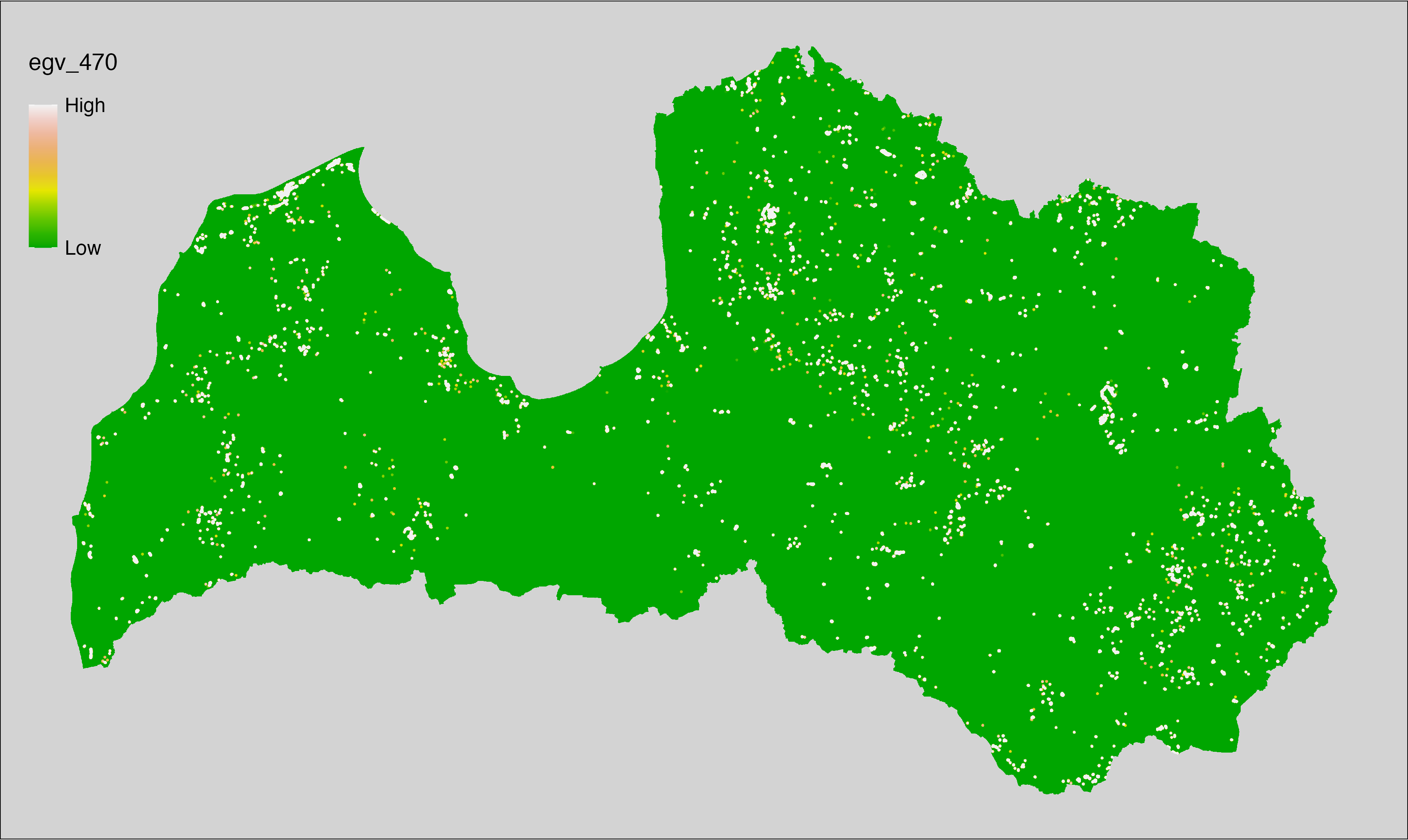
6.471 Wetlands_Mires_r1250
filename: Wetlands_Mires_r1250.tif
layername: egv_471
English name: Fractional cover of Transitional Mires within the 1.25 km landscape
Latvian name: Pārejas purvu platības īpatsvars 1,25 km ainavā
Procedure: The cover fraction within a radius of 1250 m around the analysis grid cell
is calculated as the area-weighted sum of the analysis cells inside
the buffer, using the workflow egvtools::radius_function(). During the calculation of the landscape
metric, inverse distance weighted (power = 2) gap filling on the output is
applied to ensure no missing values at the edges. Then the layer is
rewritten to set its name. Finally, the layer is standardised by
subtracting the arithmetic mean and dividing by the root mean squared error.
Code
# libs ----
if(!require(terra)) {install.packages("terra"); require(terra)}
if(!require(egvtools)) {remotes::install_github("aavotins/egvtools"); require(egvtools)}
# Templates -----
template100=rast("./Templates/TemplateRasters/LV100m_10km.tif")
# radii ----
radius_function(
kvadrati_path = "./Templates/TemplateGrids/tiles/",
radii_path = "./Templates/TemplateGridPoints/tiles/",
tikls100_path = "./Templates/TemplateGrids/tikls100_sauzeme.parquet",
template_path = "./Templates/TemplateRasters/LV100m_10km.tif",
input_layers = c("./RasterGrids_100m/2024/RAW/Wetlands_Mires_cell.tif"),
layer_prefixes = c("Wetlands_Mires"),
output_dir = "./RasterGrids_100m/2024/RAW/",
n_workers = 12,
radii = c("r1250"),
radius_mode = "sparse",
extract_fun = "mean",
fill_missing = TRUE,
IDW_weight = 2,
future_max_size = 20 * 1024^3)
# Wetlands_Mires_r1250.tif egv_471
slanis=rast("./RasterGrids_100m/2024/RAW/Wetlands_Mires_r1250.tif")
names(slanis)="egv_471"
slanis2=project(slanis,template100)
writeRaster(slanis2,
"./RasterGrids_100m/2024/RAW/Wetlands_Mires_r1250.tif",
overwrite=TRUE)
# standardisation ----
if(!require(terra)) {install.packages("terra"); require(terra)}
if(!require(tidyverse)) {install.packages("tidyverse"); require(tidyverse)}
nosaukums="Wetlands_Mires_r1250.tif"
ielasisanas_cels=paste0("./RasterGrids_100m/2024/RAW/",nosaukums)
saglabasanas_cels=paste0("./RasterGrids_100m/2024/Scaled/",nosaukums)
slanis=rast(ielasisanas_cels)
videjais=global(slanis,fun="mean",na.rm=TRUE)
centrets=slanis-videjais[,1]
standartnovirze=terra::global(centrets,fun="rms",na.rm=TRUE)
merogots=centrets/standartnovirze[,1]
writeRaster(merogots,
filename=saglabasanas_cels,
overwrite=TRUE)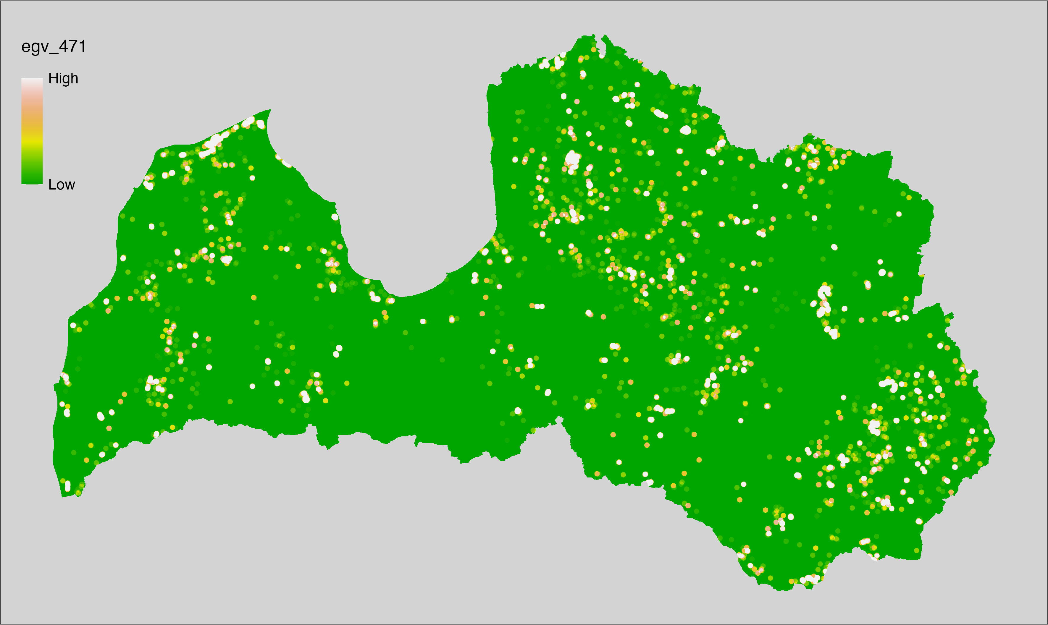
6.472 Wetlands_Mires_r3000
filename: Wetlands_Mires_r3000.tif
layername: egv_472
English name: Fractional cover of Transitional Mires within the 3 km landscape
Latvian name: Pārejas purvu platības īpatsvars 3 km ainavā
Procedure: The cover fraction within a radius of 3000 m around the analysis grid cell
is calculated as the area-weighted sum of the analysis cells inside
the buffer, using the workflow egvtools::radius_function(). During the calculation of the landscape
metric, inverse distance weighted (power = 2) gap filling on the output is
applied to ensure no missing values at the edges. Then the layer is
rewritten to set its name. Finally, the layer is standardised by
subtracting the arithmetic mean and dividing by the root mean squared error.
Code
# libs ----
if(!require(terra)) {install.packages("terra"); require(terra)}
if(!require(egvtools)) {remotes::install_github("aavotins/egvtools"); require(egvtools)}
# Templates -----
template100=rast("./Templates/TemplateRasters/LV100m_10km.tif")
# radii ----
radius_function(
kvadrati_path = "./Templates/TemplateGrids/tiles/",
radii_path = "./Templates/TemplateGridPoints/tiles/",
tikls100_path = "./Templates/TemplateGrids/tikls100_sauzeme.parquet",
template_path = "./Templates/TemplateRasters/LV100m_10km.tif",
input_layers = c("./RasterGrids_100m/2024/RAW/Wetlands_Mires_cell.tif"),
layer_prefixes = c("Wetlands_Mires"),
output_dir = "./RasterGrids_100m/2024/RAW/",
n_workers = 12,
radii = c("r3000"),
radius_mode = "sparse",
extract_fun = "mean",
fill_missing = TRUE,
IDW_weight = 2,
future_max_size = 20 * 1024^3)
# Wetlands_Mires_r3000.tif egv_472
slanis=rast("./RasterGrids_100m/2024/RAW/Wetlands_Mires_r3000.tif")
names(slanis)="egv_472"
slanis2=project(slanis,template100)
writeRaster(slanis2,
"./RasterGrids_100m/2024/RAW/Wetlands_Mires_r3000.tif",
overwrite=TRUE)
# standardisation ----
if(!require(terra)) {install.packages("terra"); require(terra)}
if(!require(tidyverse)) {install.packages("tidyverse"); require(tidyverse)}
nosaukums="Wetlands_Mires_r3000.tif"
ielasisanas_cels=paste0("./RasterGrids_100m/2024/RAW/",nosaukums)
saglabasanas_cels=paste0("./RasterGrids_100m/2024/Scaled/",nosaukums)
slanis=rast(ielasisanas_cels)
videjais=global(slanis,fun="mean",na.rm=TRUE)
centrets=slanis-videjais[,1]
standartnovirze=terra::global(centrets,fun="rms",na.rm=TRUE)
merogots=centrets/standartnovirze[,1]
writeRaster(merogots,
filename=saglabasanas_cels,
overwrite=TRUE)
6.473 Wetlands_Mires_r10000
filename: Wetlands_Mires_r10000.tif
layername: egv_473
English name: Fractional cover of Transitional Mires within the 10 km landscape
Latvian name: Pārejas purvu platības īpatsvars 10 km ainavā
Procedure: The cover fraction within a radius of 10000 m around the analysis grid cell
is calculated as the area-weighted sum of the analysis cells inside
the buffer, using the workflow egvtools::radius_function(). During the calculation of the landscape
metric, inverse distance weighted (power = 2) gap filling on the output is
applied to ensure no missing values at the edges. Then the layer is
rewritten to set its name. Finally, the layer is standardised by
subtracting the arithmetic mean and dividing by the root mean squared error.
Code
# libs ----
if(!require(terra)) {install.packages("terra"); require(terra)}
if(!require(egvtools)) {remotes::install_github("aavotins/egvtools"); require(egvtools)}
# Templates -----
template100=rast("./Templates/TemplateRasters/LV100m_10km.tif")
# radii ----
radius_function(
kvadrati_path = "./Templates/TemplateGrids/tiles/",
radii_path = "./Templates/TemplateGridPoints/tiles/",
tikls100_path = "./Templates/TemplateGrids/tikls100_sauzeme.parquet",
template_path = "./Templates/TemplateRasters/LV100m_10km.tif",
input_layers = c("./RasterGrids_100m/2024/RAW/Wetlands_Mires_cell.tif"),
layer_prefixes = c("Wetlands_Mires"),
output_dir = "./RasterGrids_100m/2024/RAW/",
n_workers = 12,
radii = c("r10000"),
radius_mode = "sparse",
extract_fun = "mean",
fill_missing = TRUE,
IDW_weight = 2,
future_max_size = 20 * 1024^3)
# Wetlands_Mires_r10000.tif egv_473
slanis=rast("./RasterGrids_100m/2024/RAW/Wetlands_Mires_r10000.tif")
names(slanis)="egv_473"
slanis2=project(slanis,template100)
writeRaster(slanis2,
"./RasterGrids_100m/2024/RAW/Wetlands_Mires_r10000.tif",
overwrite=TRUE)
# standardisation ----
if(!require(terra)) {install.packages("terra"); require(terra)}
if(!require(tidyverse)) {install.packages("tidyverse"); require(tidyverse)}
nosaukums="Wetlands_Mires_r10000.tif"
ielasisanas_cels=paste0("./RasterGrids_100m/2024/RAW/",nosaukums)
saglabasanas_cels=paste0("./RasterGrids_100m/2024/Scaled/",nosaukums)
slanis=rast(ielasisanas_cels)
videjais=global(slanis,fun="mean",na.rm=TRUE)
centrets=slanis-videjais[,1]
standartnovirze=terra::global(centrets,fun="rms",na.rm=TRUE)
merogots=centrets/standartnovirze[,1]
writeRaster(merogots,
filename=saglabasanas_cels,
overwrite=TRUE)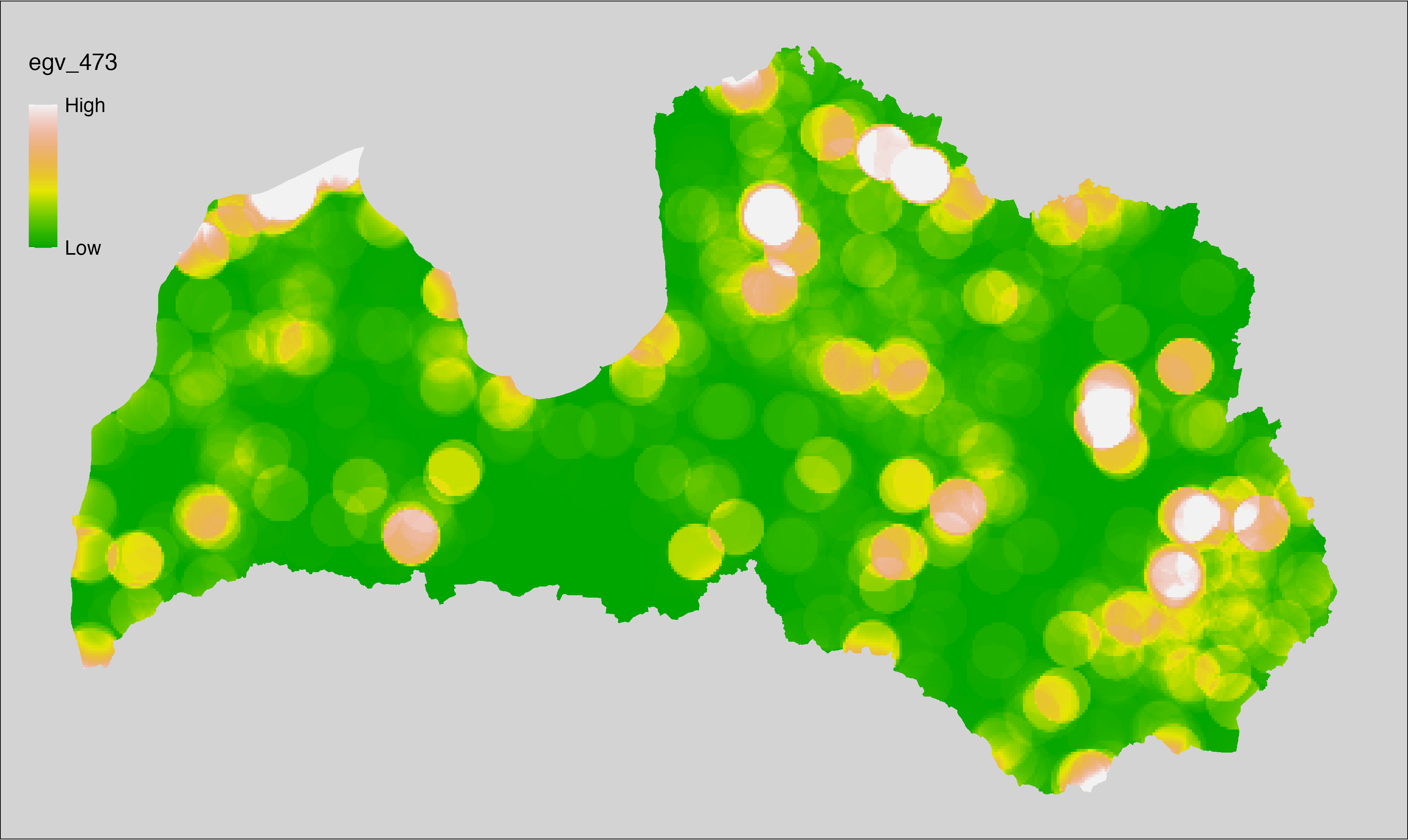
6.474 Wetlands_ReedSedgeRushBeds_cell
filename: Wetlands_ReedSedgeRushBeds_cell.tif
layername: egv_474
English name: Fractional cover of Reed-, Sedge-, Rush-, Beds within the analysis cell (1 ha)
Latvian name: Niedrāju, grīslāju, meldrāju platības īpatsvars analīzes šūnā (1 ha)
Procedure: First, the reed, sedge and rush beds from the Landscape
classification are selected (value 720 is reclassified to value 1;
all others are set to 0). The resulting layer
is then aggregated to EGV resolution using the workflow egvtools::input2egv(), which
calculates the arithmetic mean to determine the cover fraction. During
aggregation, inverse distance weighted (power = 2) gap filling on the output is
applied to ensure no missing values at the edges. Finally, the layer is
standardised by subtracting the arithmetic mean and dividing by the root mean squared
error.
Code
# libs ----
if(!require(egvtools)) {remotes::install_github("aavotins/egvtools"); require(egvtools)}
if(!require(terra)) {install.packages("terra"); require(terra)}
if(!require(sf)) {install.packages("sf"); require(sf)}
if(!require(tidyverse)) {install.packages("tidyverse"); require(tidyverse)}
if(!require(sfarrow)) {install.packages("sfarrow"); require(sfarrow)}
if(!require(readxl)) {install.packages("readxl"); require(readxl)}
if(!require(raster)) {install.packages("raster"); require(raster)}
if(!require(fasterize)) {install.packages("fasterize"); require(fasterize)}
# templates ----
template100=rast("./Templates/TemplateRasters/LV100m_10km.tif")
template10=rast("./Templates/TemplateRasters/LV10m_10km.tif")
rastrs10=raster(template10)
nulls10=rast("./Templates/TemplateRasters/nulls_LV10m_10km.tif")
nulls100=rast("./Templates/TemplateRasters/nulls_LV100m_10km.tif")
# codes ----
kodi=read_excel("./Geodata/2024/LAD/KulturuKodi_2024.xlsx")
kodi$kods=as.character(kodi$kods)
# LAD ----
lad=sfarrow::st_read_parquet("./Geodata/2024/LAD/Lauki_2024.parquet")
lad$yes=1
lad=lad %>%
left_join(kodi,by=c("PRODUCT_CODE"="kods"))
# simple landscape ----
simple_landscape=rast("RasterGrids_10m/2024/Ainava_vienk_mask.tif")
# Wetlands_ReedSedgeRushBeds_cell.tif egv_474 ----
reedsedgerush=ifel(simple_landscape==720,1,0)
i2e_rez=egvtools::input2egv(input=reedsedgerush,
egv_template= "./Templates/TemplateRasters/LV100m_10km.tif",
summary_function = "average",
missing_job = "FillOutput",
outlocation = "./RasterGrids_100m/2024/RAW/",
outfilename = "Wetlands_ReedSedgeRushBeds_cell.tif",
layername = "egv_474",
idw_weight = 2,
plot_gaps = FALSE,plot_final = TRUE)
i2e_rez
rm(reedsedgerush)
rm(i2e_rez)
rm(simple_landscape)
# standardisation ----
if(!require(terra)) {install.packages("terra"); require(terra)}
if(!require(tidyverse)) {install.packages("tidyverse"); require(tidyverse)}
nosaukums="Wetlands_ReedSedgeRushBeds_cell.tif"
ielasisanas_cels=paste0("./RasterGrids_100m/2024/RAW/",nosaukums)
saglabasanas_cels=paste0("./RasterGrids_100m/2024/Scaled/",nosaukums)
slanis=rast(ielasisanas_cels)
videjais=global(slanis,fun="mean",na.rm=TRUE)
centrets=slanis-videjais[,1]
standartnovirze=terra::global(centrets,fun="rms",na.rm=TRUE)
merogots=centrets/standartnovirze[,1]
writeRaster(merogots,
filename=saglabasanas_cels,
overwrite=TRUE)
6.475 Wetlands_ReedSedgeRushBeds_r500
filename: Wetlands_ReedSedgeRushBeds_r500.tif
layername: egv_475
English name: Fractional cover of Reed-, Sedge-, Rush-, Beds within the 0.5 km landscape
Latvian name: Niedrāju, grīslāju, meldrāju platības īpatsvars 0,5 km ainavā
Procedure: The cover fraction within a radius of 500 m around the analysis grid cell is
calculated as the area-weighted sum of the analysis cells inside the
buffer, using the workflow egvtools::radius_function(). During the calculation of the landscape metric,
inverse distance weighted (power = 2) gap filling on the output is applied
to ensure no missing values at the edges. Then the layer is rewritten to set
its name. Finally, the layer is standardised by subtracting the arithmetic
mean and dividing by the root mean squared error.
Code
# libs ----
if(!require(terra)) {install.packages("terra"); require(terra)}
if(!require(egvtools)) {remotes::install_github("aavotins/egvtools"); require(egvtools)}
# Templates -----
template100=rast("./Templates/TemplateRasters/LV100m_10km.tif")
# radii ----
radius_function(
kvadrati_path = "./Templates/TemplateGrids/tiles/",
radii_path = "./Templates/TemplateGridPoints/tiles/",
tikls100_path = "./Templates/TemplateGrids/tikls100_sauzeme.parquet",
template_path = "./Templates/TemplateRasters/LV100m_10km.tif",
input_layers = c("./RasterGrids_100m/2024/RAW/Wetlands_ReedSedgeRushBeds_cell.tif"),
layer_prefixes = c("Wetlands_ReedSedgeRushBeds"),
output_dir = "./RasterGrids_100m/2024/RAW/",
n_workers = 12,
radii = c("r500"),
radius_mode = "sparse",
extract_fun = "mean",
fill_missing = TRUE,
IDW_weight = 2,
future_max_size = 20 * 1024^3)
# Wetlands_ReedSedgeRushBeds_r500.tif egv_475
slanis=rast("./RasterGrids_100m/2024/RAW/Wetlands_ReedSedgeRushBeds_r500.tif")
names(slanis)="egv_475"
slanis2=project(slanis,template100)
writeRaster(slanis2,
"./RasterGrids_100m/2024/RAW/Wetlands_ReedSedgeRushBeds_r500.tif",
overwrite=TRUE)
# standardisation ----
if(!require(terra)) {install.packages("terra"); require(terra)}
if(!require(tidyverse)) {install.packages("tidyverse"); require(tidyverse)}
nosaukums="Wetlands_ReedSedgeRushBeds_r500.tif"
ielasisanas_cels=paste0("./RasterGrids_100m/2024/RAW/",nosaukums)
saglabasanas_cels=paste0("./RasterGrids_100m/2024/Scaled/",nosaukums)
slanis=rast(ielasisanas_cels)
videjais=global(slanis,fun="mean",na.rm=TRUE)
centrets=slanis-videjais[,1]
standartnovirze=terra::global(centrets,fun="rms",na.rm=TRUE)
merogots=centrets/standartnovirze[,1]
writeRaster(merogots,
filename=saglabasanas_cels,
overwrite=TRUE)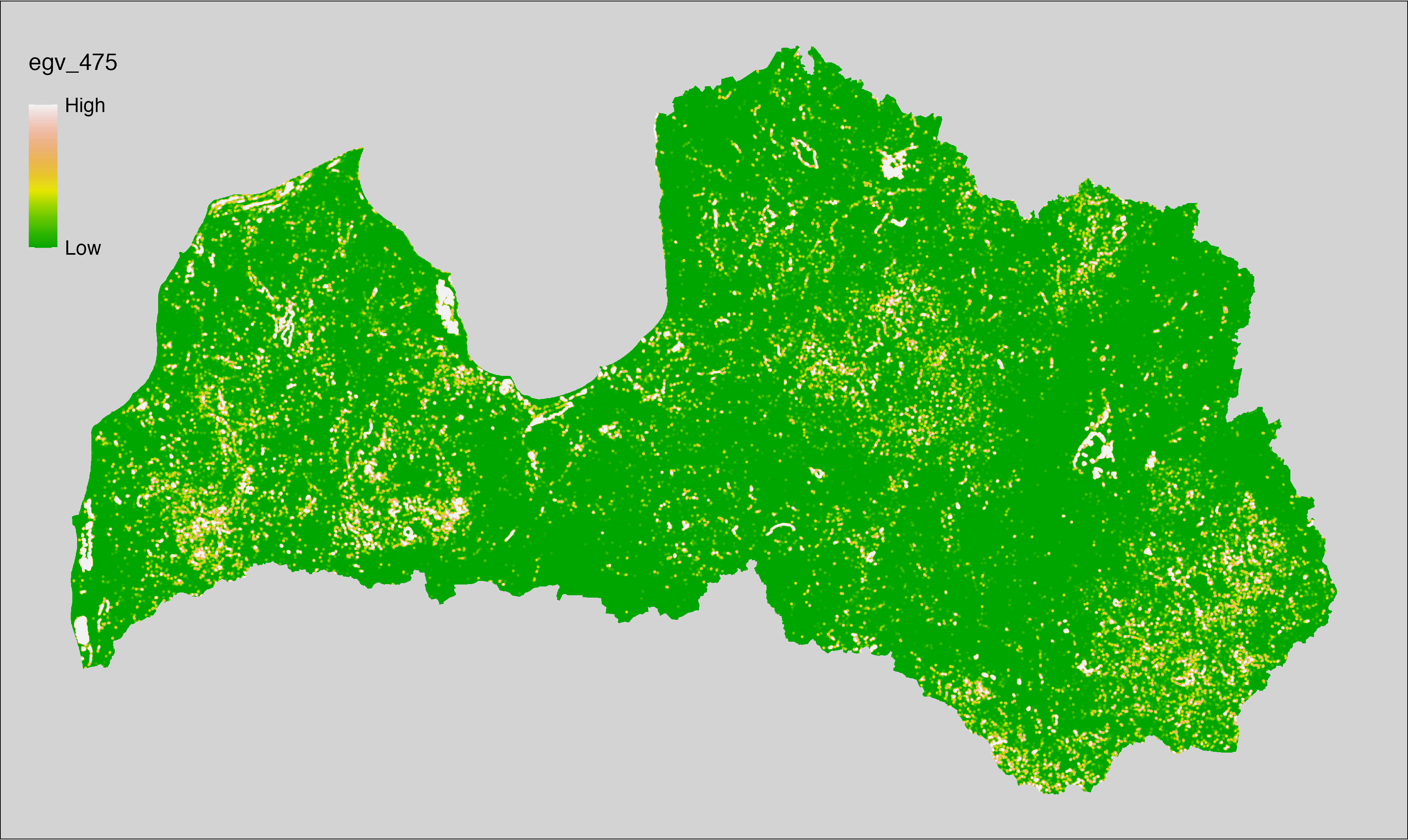
6.476 Wetlands_ReedSedgeRushBeds_r1250
filename: Wetlands_ReedSedgeRushBeds_r1250.tif
layername: egv_476
English name: Fractional cover of Reed-, Sedge-, Rush-, Beds within the 1.25 km landscape
Latvian name: Niedrāju, grīslāju, meldrāju platības īpatsvars 1,25 km ainavā
Procedure: The cover fraction within a radius of 1250 m around the analysis grid cell
is calculated as the area-weighted sum of the analysis cells inside
the buffer, using the workflow egvtools::radius_function(). During the calculation of the landscape
metric, inverse distance weighted (power = 2) gap filling on the output is
applied to ensure no missing values at the edges. Then the layer is
rewritten to set its name. Finally, the layer is standardised by
subtracting the arithmetic mean and dividing by the root mean squared error.
Code
# libs ----
if(!require(terra)) {install.packages("terra"); require(terra)}
if(!require(egvtools)) {remotes::install_github("aavotins/egvtools"); require(egvtools)}
# Templates -----
template100=rast("./Templates/TemplateRasters/LV100m_10km.tif")
# radii ----
radius_function(
kvadrati_path = "./Templates/TemplateGrids/tiles/",
radii_path = "./Templates/TemplateGridPoints/tiles/",
tikls100_path = "./Templates/TemplateGrids/tikls100_sauzeme.parquet",
template_path = "./Templates/TemplateRasters/LV100m_10km.tif",
input_layers = c("./RasterGrids_100m/2024/RAW/Wetlands_ReedSedgeRushBeds_cell.tif"),
layer_prefixes = c("Wetlands_ReedSedgeRushBeds"),
output_dir = "./RasterGrids_100m/2024/RAW/",
n_workers = 12,
radii = c("r1250"),
radius_mode = "sparse",
extract_fun = "mean",
fill_missing = TRUE,
IDW_weight = 2,
future_max_size = 20 * 1024^3)
# Wetlands_ReedSedgeRushBeds_r1250.tif egv_476
slanis=rast("./RasterGrids_100m/2024/RAW/Wetlands_ReedSedgeRushBeds_r1250.tif")
names(slanis)="egv_476"
slanis2=project(slanis,template100)
writeRaster(slanis2,
"./RasterGrids_100m/2024/RAW/Wetlands_ReedSedgeRushBeds_r1250.tif",
overwrite=TRUE)
# standardisation ----
if(!require(terra)) {install.packages("terra"); require(terra)}
if(!require(tidyverse)) {install.packages("tidyverse"); require(tidyverse)}
nosaukums="Wetlands_ReedSedgeRushBeds_r1250.tif"
ielasisanas_cels=paste0("./RasterGrids_100m/2024/RAW/",nosaukums)
saglabasanas_cels=paste0("./RasterGrids_100m/2024/Scaled/",nosaukums)
slanis=rast(ielasisanas_cels)
videjais=global(slanis,fun="mean",na.rm=TRUE)
centrets=slanis-videjais[,1]
standartnovirze=terra::global(centrets,fun="rms",na.rm=TRUE)
merogots=centrets/standartnovirze[,1]
writeRaster(merogots,
filename=saglabasanas_cels,
overwrite=TRUE)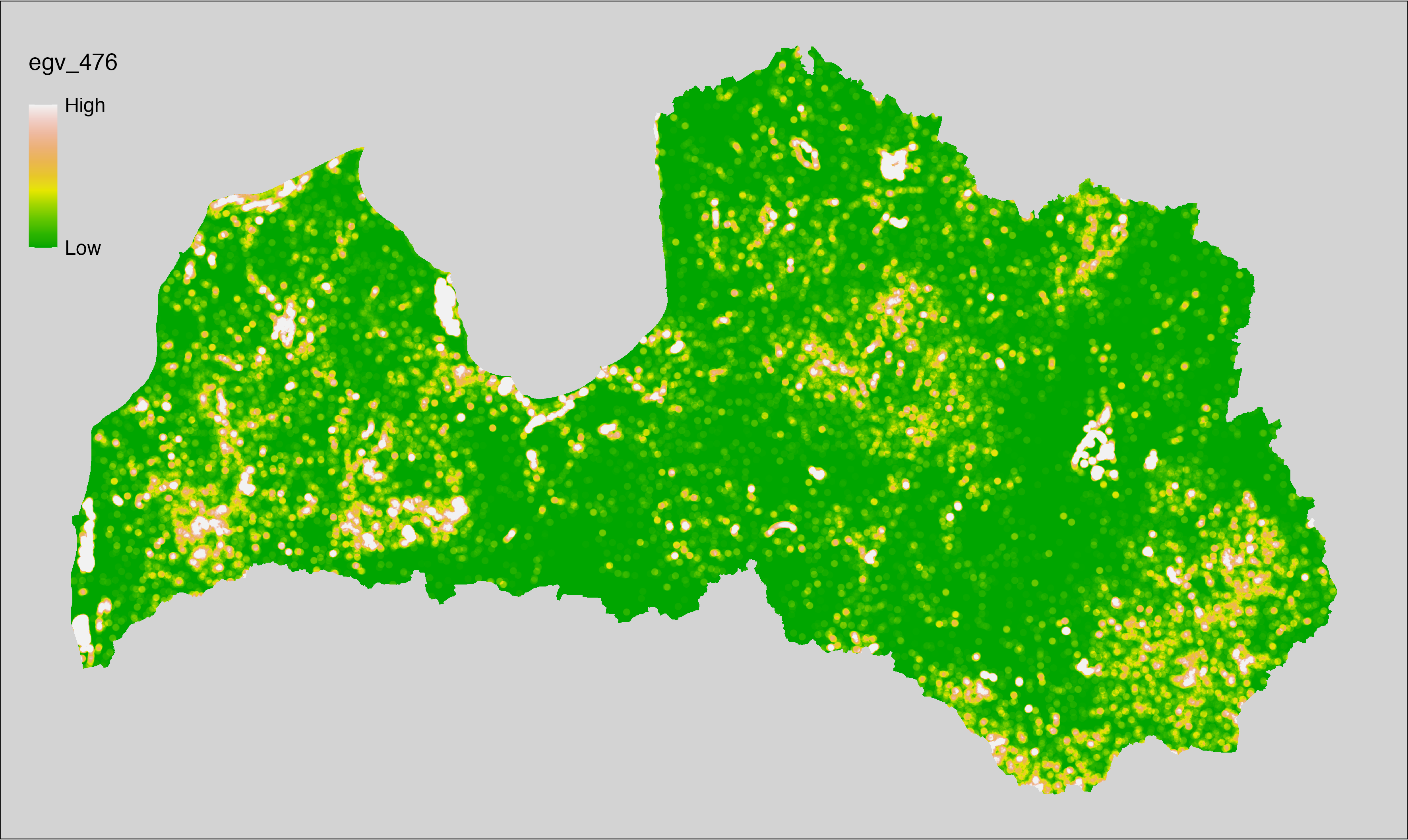
6.477 Wetlands_ReedSedgeRushBeds_r3000
filename: Wetlands_ReedSedgeRushBeds_r3000.tif
layername: egv_477
English name: Fractional cover of Reed-, Sedge-, Rush-, Beds within the 3 km landscape
Latvian name: Niedrāju, grīslāju, meldrāju platības īpatsvars 3 km ainavā
Procedure: The cover fraction within a radius of 3000 m around the analysis grid cell
is calculated as the area-weighted sum of the analysis cells inside
the buffer, using the workflow egvtools::radius_function(). During the calculation of the landscape
metric, inverse distance weighted (power = 2) gap filling on the output is
applied to ensure no missing values at the edges. Then the layer is
rewritten to set its name. Finally, the layer is standardised by
subtracting the arithmetic mean and dividing by the root mean squared error.
Code
# libs ----
if(!require(terra)) {install.packages("terra"); require(terra)}
if(!require(egvtools)) {remotes::install_github("aavotins/egvtools"); require(egvtools)}
# Templates -----
template100=rast("./Templates/TemplateRasters/LV100m_10km.tif")
# radii ----
radius_function(
kvadrati_path = "./Templates/TemplateGrids/tiles/",
radii_path = "./Templates/TemplateGridPoints/tiles/",
tikls100_path = "./Templates/TemplateGrids/tikls100_sauzeme.parquet",
template_path = "./Templates/TemplateRasters/LV100m_10km.tif",
input_layers = c("./RasterGrids_100m/2024/RAW/Wetlands_ReedSedgeRushBeds_cell.tif"),
layer_prefixes = c("Wetlands_ReedSedgeRushBeds"),
output_dir = "./RasterGrids_100m/2024/RAW/",
n_workers = 12,
radii = c("r3000"),
radius_mode = "sparse",
extract_fun = "mean",
fill_missing = TRUE,
IDW_weight = 2,
future_max_size = 20 * 1024^3)
# Wetlands_ReedSedgeRushBeds_r3000.tif egv_477
slanis=rast("./RasterGrids_100m/2024/RAW/Wetlands_ReedSedgeRushBeds_r3000.tif")
names(slanis)="egv_477"
slanis2=project(slanis,template100)
writeRaster(slanis2,
"./RasterGrids_100m/2024/RAW/Wetlands_ReedSedgeRushBeds_r3000.tif",
overwrite=TRUE)
# standardisation ----
if(!require(terra)) {install.packages("terra"); require(terra)}
if(!require(tidyverse)) {install.packages("tidyverse"); require(tidyverse)}
nosaukums="Wetlands_ReedSedgeRushBeds_r3000.tif"
ielasisanas_cels=paste0("./RasterGrids_100m/2024/RAW/",nosaukums)
saglabasanas_cels=paste0("./RasterGrids_100m/2024/Scaled/",nosaukums)
slanis=rast(ielasisanas_cels)
videjais=global(slanis,fun="mean",na.rm=TRUE)
centrets=slanis-videjais[,1]
standartnovirze=terra::global(centrets,fun="rms",na.rm=TRUE)
merogots=centrets/standartnovirze[,1]
writeRaster(merogots,
filename=saglabasanas_cels,
overwrite=TRUE)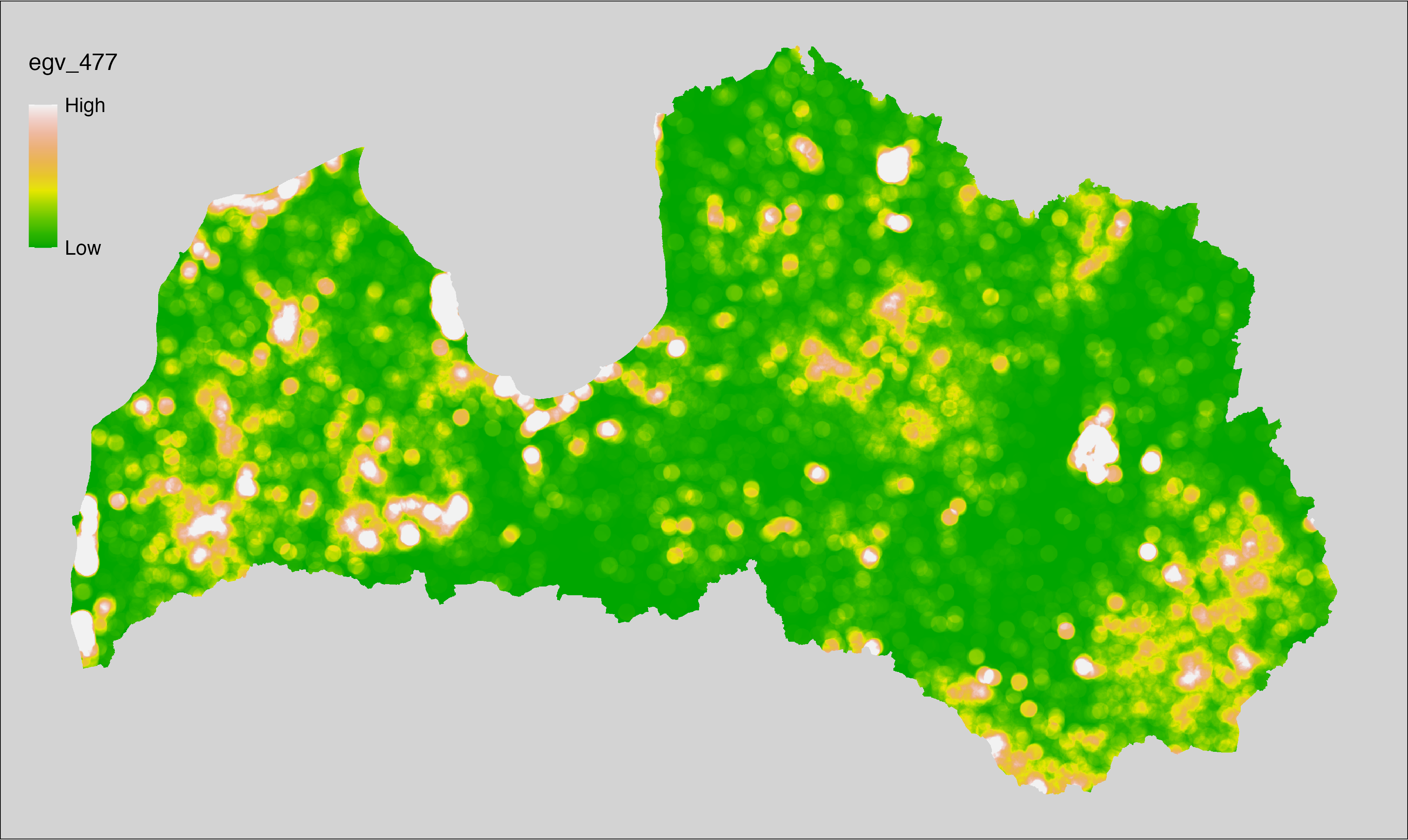
6.478 Wetlands_ReedSedgeRushBeds_r10000
filename: Wetlands_ReedSedgeRushBeds_r10000.tif
layername: egv_478
English name: Fractional cover of Reed-, Sedge-, Rush-, Beds within the 10 km landscape
Latvian name: Niedrāju, grīslāju, meldrāju platības īpatsvars 10 km ainavā
Procedure: The cover fraction within a radius of 10000 m around the analysis grid cell
is calculated as the area-weighted sum of the analysis cells inside
the buffer, using the workflow egvtools::radius_function(). During the calculation of the landscape
metric, inverse distance weighted (power = 2) gap filling on the output is
applied to ensure no missing values at the edges. Then the layer is
rewritten to set its name. Finally, the layer is standardised by
subtracting the arithmetic mean and dividing by the root mean squared error.
Code
# libs ----
if(!require(terra)) {install.packages("terra"); require(terra)}
if(!require(egvtools)) {remotes::install_github("aavotins/egvtools"); require(egvtools)}
# Templates -----
template100=rast("./Templates/TemplateRasters/LV100m_10km.tif")
# radii ----
radius_function(
kvadrati_path = "./Templates/TemplateGrids/tiles/",
radii_path = "./Templates/TemplateGridPoints/tiles/",
tikls100_path = "./Templates/TemplateGrids/tikls100_sauzeme.parquet",
template_path = "./Templates/TemplateRasters/LV100m_10km.tif",
input_layers = c("./RasterGrids_100m/2024/RAW/Wetlands_ReedSedgeRushBeds_cell.tif"),
layer_prefixes = c("Wetlands_ReedSedgeRushBeds"),
output_dir = "./RasterGrids_100m/2024/RAW/",
n_workers = 12,
radii = c("r10000"),
radius_mode = "sparse",
extract_fun = "mean",
fill_missing = TRUE,
IDW_weight = 2,
future_max_size = 20 * 1024^3)
# Wetlands_ReedSedgeRushBeds_r10000.tif egv_478
slanis=rast("./RasterGrids_100m/2024/RAW/Wetlands_ReedSedgeRushBeds_r10000.tif")
names(slanis)="egv_478"
slanis2=project(slanis,template100)
writeRaster(slanis2,
"./RasterGrids_100m/2024/RAW/Wetlands_ReedSedgeRushBeds_r10000.tif",
overwrite=TRUE)
# standardisation ----
if(!require(terra)) {install.packages("terra"); require(terra)}
if(!require(tidyverse)) {install.packages("tidyverse"); require(tidyverse)}
nosaukums="Wetlands_ReedSedgeRushBeds_r10000.tif"
ielasisanas_cels=paste0("./RasterGrids_100m/2024/RAW/",nosaukums)
saglabasanas_cels=paste0("./RasterGrids_100m/2024/Scaled/",nosaukums)
slanis=rast(ielasisanas_cels)
videjais=global(slanis,fun="mean",na.rm=TRUE)
centrets=slanis-videjais[,1]
standartnovirze=terra::global(centrets,fun="rms",na.rm=TRUE)
merogots=centrets/standartnovirze[,1]
writeRaster(merogots,
filename=saglabasanas_cels,
overwrite=TRUE)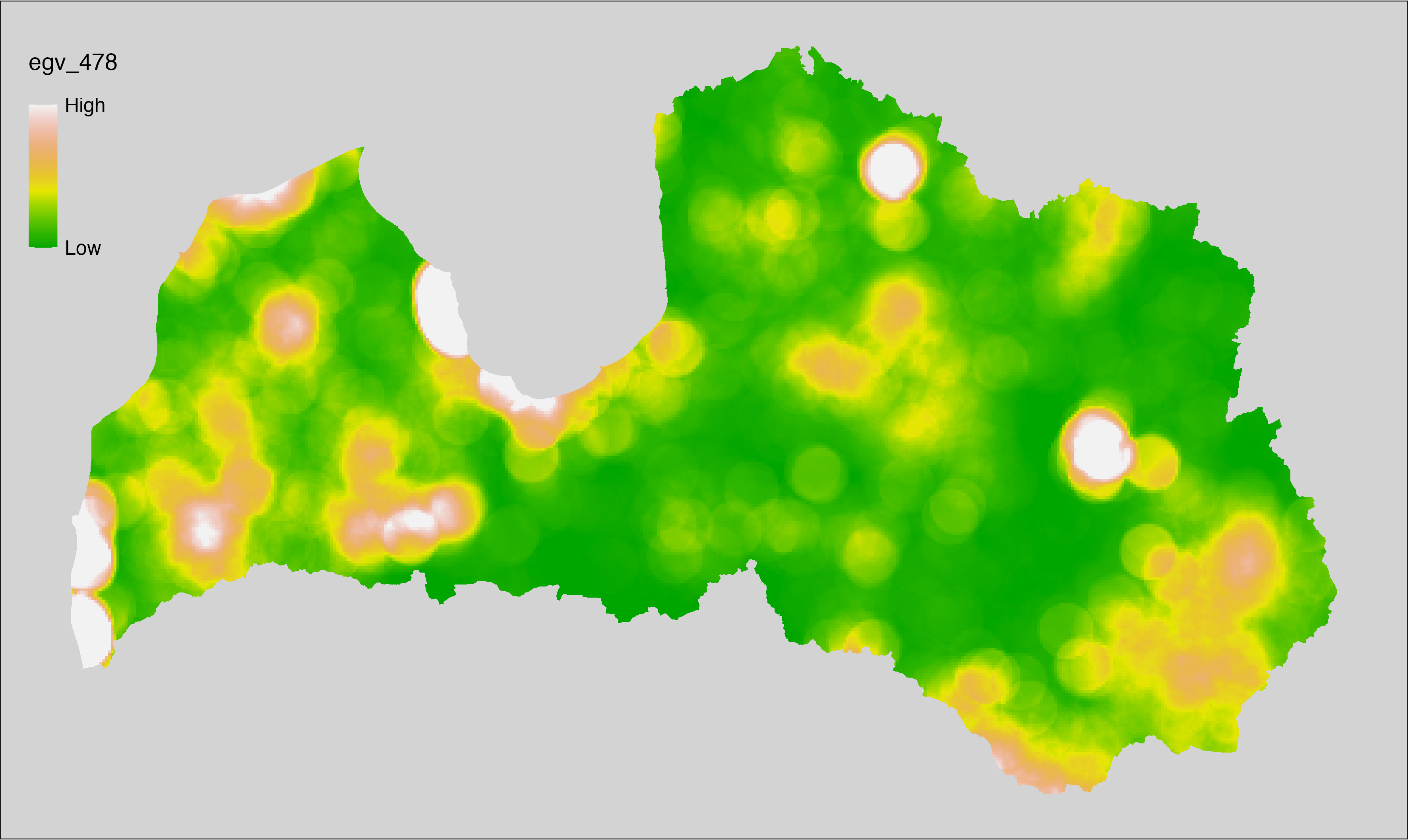
6.479 EO_NDMI-LYmed-average_cell
filename: EO_NDMI-LYmed-average_cell.tif
layername: egv_479
English name: Median vegetation water content index (NDMI) for the last year within the analysis cell (1 ha)
Latvian name: Mediānā pēdējā gada ūdens satura veģetācijā indeksa (NDMI) vērtība analīzes šūnā (1 ha)
Procedure: Directly follows preprocessing. The arithmetic mean value
at the analysis cell is calculated using the workflow egvtools::input2egv(). To
protect against potential data loss at edge cells, inverse distance
weighted (power = 2) gap filling is implemented. Finally, the layer is
standardised by subtracting the arithmetic mean and
dividing by the root mean squared error. The “last year” is 2024.
Code
# libs ----
if(!require(egvtools)) {remotes::install_github("aavotins/egvtools"); require(egvtools)}
# EO_NDMI-LYmed-average_cell.tif ----
egvrez=input2egv(input="./Geodata/2024/S2indices/Mosaics/EO_NDMI-LYmedian.tif",
egv_template= "./Templates/TemplateRasters/LV100m_10km.tif",
summary_function = "average",
missing_job = "FillOutput",
outlocation = "./RasterGrids_100m/2024/RAW/",
outfilename = "EO_NDMI-LYmed-average_cell.tif",
layername = "egv_479",
idw_weight = 2,
plot_gaps = FALSE,
plot_final = FALSE)
egvrez
# standardisation ----
if(!require(terra)) {install.packages("terra"); require(terra)}
if(!require(tidyverse)) {install.packages("tidyverse"); require(tidyverse)}
nosaukums="EO_NDMI-LYmed-average_cell.tif"
ielasisanas_cels=paste0("./RasterGrids_100m/2024/RAW/",nosaukums)
saglabasanas_cels=paste0("./RasterGrids_100m/2024/Scaled/",nosaukums)
slanis=rast(ielasisanas_cels)
videjais=global(slanis,fun="mean",na.rm=TRUE)
centrets=slanis-videjais[,1]
standartnovirze=terra::global(centrets,fun="rms",na.rm=TRUE)
merogots=centrets/standartnovirze[,1]
writeRaster(merogots,
filename=saglabasanas_cels,
overwrite=TRUE)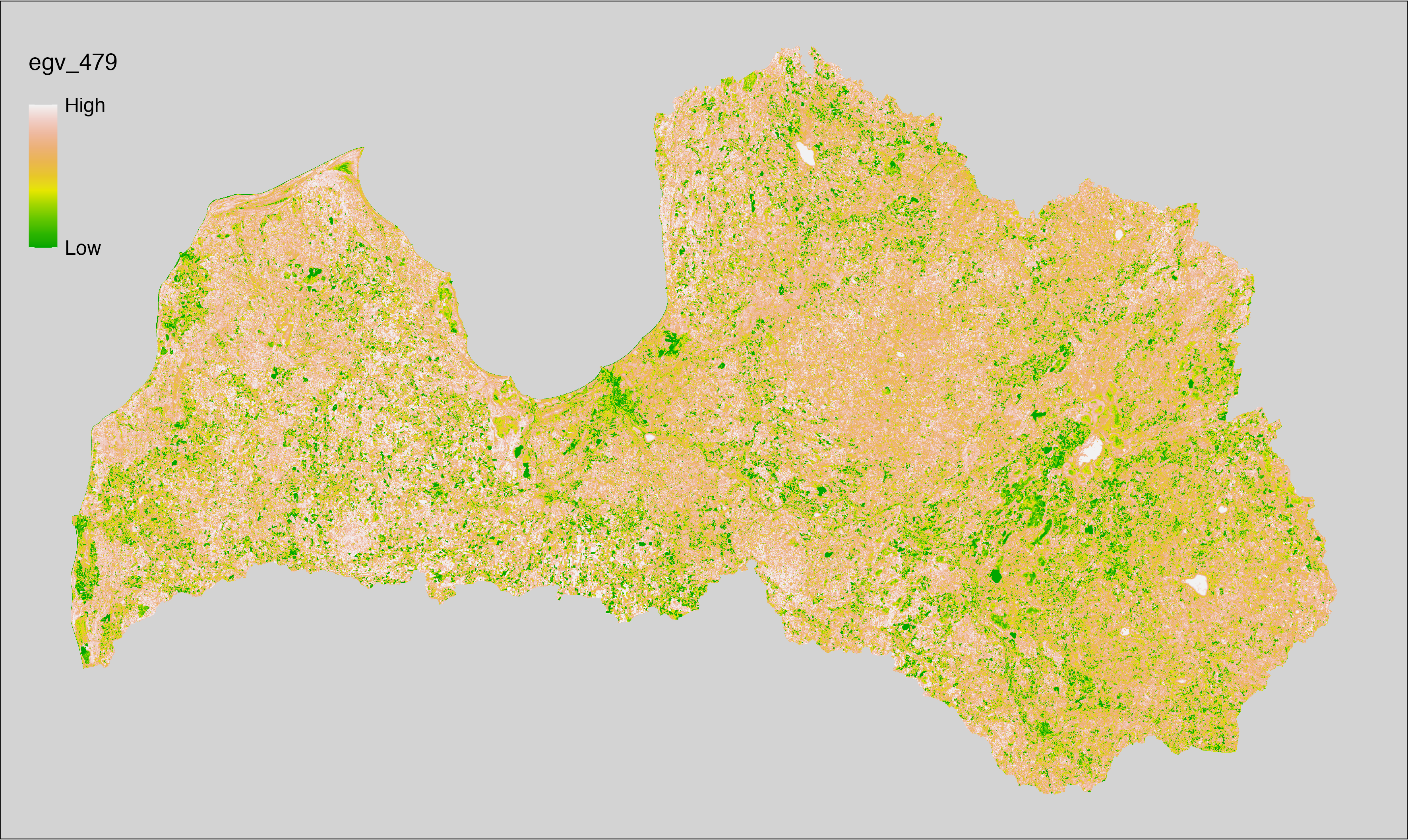
6.480 EO_NDMI-LYmedian-iqr_cell
filename: EO_NDMI-LYmedian-iqr_cell.tif
layername: egv_480
English name: Spatial variability of last year’s median vegetation water content index (NDMI) within the analysis cell (1 ha)
Latvian name: Telpiskā variabilitāte pēdējā gada mediānajai ūdens satura veģetācijā indeksa (NDMI) vērtībai analīzes šūnā (1 ha)
Procedure: Directly follows preprocessing. The
workflow egvtools::input2egv() is used to calculate Q1 and Q3 for every cell.
To protect against potential data loss at the edges, inverse distance
weighted (power = 2) gap filling is implemented. Next, Q1 is subtracted from Q3.
Finally, the layer is standardised by subtracting the arithmetic mean and
dividing by the root mean squared error. The “last year” is 2024.
Code
# libs ----
if(!require(egvtools)) {remotes::install_github("aavotins/egvtools"); require(egvtools)}
# EO_NDMI-LYmedian-iqr_cell.tif ----
p25rez=input2egv(input="./Geodata/2024/S2indices/Mosaics/EO_NDMI-LYmedian.tif",
egv_template= "./Templates/TemplateRasters/LV100m_10km.tif",
summary_function = "q1",
missing_job = "FillOutput",
outlocation = "./RasterGrids_100m/2024/",
outfilename = "draza_p25.tif",
layername = "egv_480",
idw_weight = 2,
plot_gaps = FALSE,
plot_final = FALSE)
p25rez_r=rast("./RasterGrids_100m/2024/draza_p25.tif")
p75rez=input2egv(input="./Geodata/2024/S2indices/Mosaics/EO_NDMI-LYmedian.tif",
egv_template= "./Templates/TemplateRasters/LV100m_10km.tif",
summary_function = "q3",
missing_job = "FillOutput",
outlocation = "./RasterGrids_100m/2024/",
outfilename = "draza_p75.tif",
layername = "egv_480",
idw_weight = 2,
plot_gaps = FALSE,
plot_final = FALSE)
p75rez_r=rast("./RasterGrids_100m/2024/draza_p75.tif")
iqr_rez=p75rez_r-p25rez_r
iqr_rez
plot(iqr_rez)
writeRaster(iqr_rez,
"./RasterGrids_100m/2024/RAW/EO_NDMI-LYmedian-iqr_cell.tif",
overwrite=TRUE)
unlink("./RasterGrids_100m/2024/draza_p75.tif")
unlink("./RasterGrids_100m/2024/draza_p25.tif")
# standardisation ----
if(!require(terra)) {install.packages("terra"); require(terra)}
if(!require(tidyverse)) {install.packages("tidyverse"); require(tidyverse)}
nosaukums="EO_NDMI-LYmedian-iqr_cell.tif"
ielasisanas_cels=paste0("./RasterGrids_100m/2024/RAW/",nosaukums)
saglabasanas_cels=paste0("./RasterGrids_100m/2024/Scaled/",nosaukums)
slanis=rast(ielasisanas_cels)
videjais=global(slanis,fun="mean",na.rm=TRUE)
centrets=slanis-videjais[,1]
standartnovirze=terra::global(centrets,fun="rms",na.rm=TRUE)
merogots=centrets/standartnovirze[,1]
writeRaster(merogots,
filename=saglabasanas_cels,
overwrite=TRUE)
6.481 EO_NDMI-STiqr-median_cell
filename: EO_NDMI-STiqr-median_cell.tif
layername: egv_481
English name: Average short-term seasonality of vegetation water content index (NDMI) within the analysis cell (1 ha)
Latvian name: Sezonalitāte pēdējo gadu vidējai ūdens satura veģetācijā indeksa (NDMI) vērtībai analīzes šūnā (1 ha)
Procedure: Directly follows preprocessing. The arithmetic mean value
at the analysis cell is calculated using the workflow egvtools::input2egv(). To
protect against potential data loss at edge cells, inverse distance
weighted (power = 2) gap filling is implemented. Finally, the layer is
standardised by subtracting the arithmetic mean and dividing by the root mean
squared error. The “short-term” refers to the last five years (2020-2024).
Code
# libs ----
if(!require(egvtools)) {remotes::install_github("aavotins/egvtools"); require(egvtools)}
# EO_NDMI-STiqr-median_cell.tif ----
egvrez=input2egv(input="./Geodata/2024/S2indices/Mosaics/EO_NDMI-STiqr.tif",
egv_template= "./Templates/TemplateRasters/LV100m_10km.tif",
summary_function = "average",
missing_job = "FillOutput",
outlocation = "./RasterGrids_100m/2024/RAW/",
outfilename = "EO_NDMI-STiqr-median_cell.tif",
layername = "egv_481",
idw_weight = 2,
plot_gaps = FALSE,
plot_final = FALSE)
egvrez
# standardisation ----
if(!require(terra)) {install.packages("terra"); require(terra)}
if(!require(tidyverse)) {install.packages("tidyverse"); require(tidyverse)}
nosaukums="EO_NDMI-STiqr-median_cell.tif"
ielasisanas_cels=paste0("./RasterGrids_100m/2024/RAW/",nosaukums)
saglabasanas_cels=paste0("./RasterGrids_100m/2024/Scaled/",nosaukums)
slanis=rast(ielasisanas_cels)
videjais=global(slanis,fun="mean",na.rm=TRUE)
centrets=slanis-videjais[,1]
standartnovirze=terra::global(centrets,fun="rms",na.rm=TRUE)
merogots=centrets/standartnovirze[,1]
writeRaster(merogots,
filename=saglabasanas_cels,
overwrite=TRUE)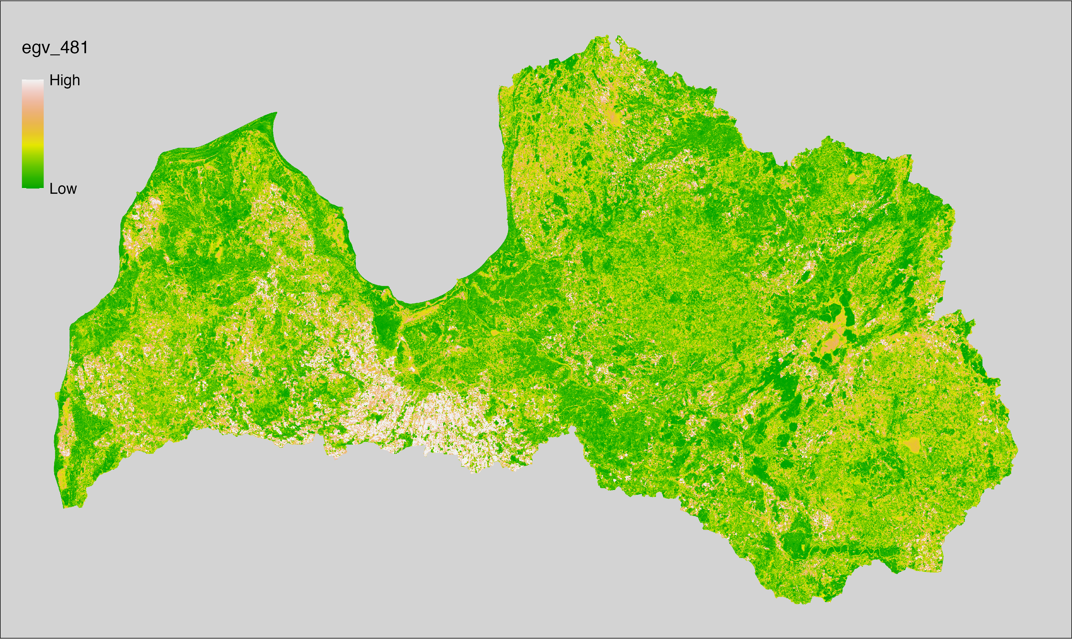
6.482 EO_NDMI-STmedian-average_cell
filename: EO_NDMI-STmedian-average_cell.tif
layername: egv_482
English name: Median short-term vegetation water content index (NDMI) within the analysis cell (1 ha)
Latvian name: Mediānā pēdējo gadu ūdens satura veģetācijā indeksa (NDMI) vērtība analīzes šūnā (1 ha)
Procedure: Directly follows preprocessing. The arithmetic mean value
at the analysis cell is calculated using the workflow egvtools::input2egv(). To
protect against potential data loss at edge cells, inverse distance
weighted (power = 2) gap filling is implemented. Finally, the layer is
standardised by subtracting the arithmetic mean and dividing by the root mean
squared error. The “short-term” refers to the last five years (2020-2024).
Code
# libs ----
if(!require(egvtools)) {remotes::install_github("aavotins/egvtools"); require(egvtools)}
# EO_NDMI-STmedian-average_cell.tif ----
egvrez=input2egv(input="./Geodata/2024/S2indices/Mosaics/EO_NDMI-STmedian.tif",
egv_template= "./Templates/TemplateRasters/LV100m_10km.tif",
summary_function = "average",
missing_job = "FillOutput",
outlocation = "./RasterGrids_100m/2024/RAW/",
outfilename = "EO_NDMI-STmedian-average_cell.tif",
layername = "egv_482",
idw_weight = 2,
plot_gaps = FALSE,
plot_final = FALSE)
egvrez
# standardisation ----
if(!require(terra)) {install.packages("terra"); require(terra)}
if(!require(tidyverse)) {install.packages("tidyverse"); require(tidyverse)}
nosaukums="EO_NDMI-STmedian-average_cell.tif"
ielasisanas_cels=paste0("./RasterGrids_100m/2024/RAW/",nosaukums)
saglabasanas_cels=paste0("./RasterGrids_100m/2024/Scaled/",nosaukums)
slanis=rast(ielasisanas_cels)
videjais=global(slanis,fun="mean",na.rm=TRUE)
centrets=slanis-videjais[,1]
standartnovirze=terra::global(centrets,fun="rms",na.rm=TRUE)
merogots=centrets/standartnovirze[,1]
writeRaster(merogots,
filename=saglabasanas_cels,
overwrite=TRUE)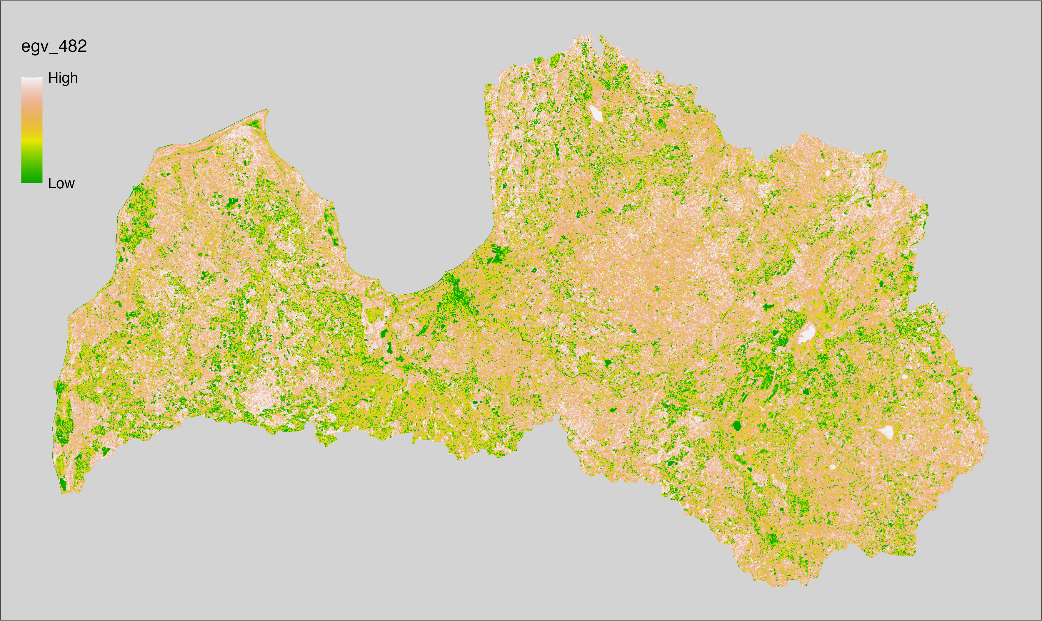
6.483 EO_NDMI-STmedian-iqr_cell
filename: EO_NDMI-STmedian-iqr_cell.tif
layername: egv_483
English name: Spatial variability of short-term median vegetation water content index (NDMI) within the analysis cell (1 ha)
Latvian name: Telpiskā variabilitāte pēdējo gadu mediānajai ūdens satura veģetācijā indeksa (NDMI) vērtībai analīzes šūnā (1 ha)
Procedure: Directly follows preprocessing. The
workflow egvtools::input2egv() is used to calculate Q1 and Q3 for every cell.
To protect against potential data loss at the edges, inverse distance
weighted (power = 2) gap filling is implemented. Next, Q1 is subtracted from Q3.
Finally, the layer is standardised by subtracting the arithmetic mean and
dividing by the root mean squared error. The “short-term” refers to the last
five years (2020-2024).
Code
# libs ----
if(!require(egvtools)) {remotes::install_github("aavotins/egvtools"); require(egvtools)}
# EO_NDMI-STmedian-iqr_cell.tif ----
p25rez=input2egv(input="./Geodata/2024/S2indices/Mosaics/EO_NDMI-STmedian.tif",
egv_template= "./Templates/TemplateRasters/LV100m_10km.tif",
summary_function = "q1",
missing_job = "FillOutput",
outlocation = "./RasterGrids_100m/2024/",
outfilename = "draza_p25.tif",
layername = "egv_483",
idw_weight = 2,
plot_gaps = FALSE,
plot_final = FALSE)
p25rez_r=rast("./RasterGrids_100m/2024/draza_p25.tif")
p75rez=input2egv(input="./Geodata/2024/S2indices/Mosaics/EO_NDMI-STmedian.tif",
egv_template= "./Templates/TemplateRasters/LV100m_10km.tif",
summary_function = "q3",
missing_job = "FillOutput",
outlocation = "./RasterGrids_100m/2024/",
outfilename = "draza_p75.tif",
layername = "egv_483",
idw_weight = 2,
plot_gaps = FALSE,
plot_final = FALSE)
p75rez_r=rast("./RasterGrids_100m/2024/draza_p75.tif")
iqr_rez=p75rez_r-p25rez_r
iqr_rez
plot(iqr_rez)
writeRaster(iqr_rez,
"./RasterGrids_100m/2024/RAW/EO_NDMI-STmedian-iqr_cell.tif",
overwrite=TRUE)
unlink("./RasterGrids_100m/2024/draza_p75.tif")
unlink("./RasterGrids_100m/2024/draza_p25.tif")
# standardisation ----
if(!require(terra)) {install.packages("terra"); require(terra)}
if(!require(tidyverse)) {install.packages("tidyverse"); require(tidyverse)}
nosaukums="EO_NDMI-STmedian-iqr_cell.tif"
ielasisanas_cels=paste0("./RasterGrids_100m/2024/RAW/",nosaukums)
saglabasanas_cels=paste0("./RasterGrids_100m/2024/Scaled/",nosaukums)
slanis=rast(ielasisanas_cels)
videjais=global(slanis,fun="mean",na.rm=TRUE)
centrets=slanis-videjais[,1]
standartnovirze=terra::global(centrets,fun="rms",na.rm=TRUE)
merogots=centrets/standartnovirze[,1]
writeRaster(merogots,
filename=saglabasanas_cels,
overwrite=TRUE)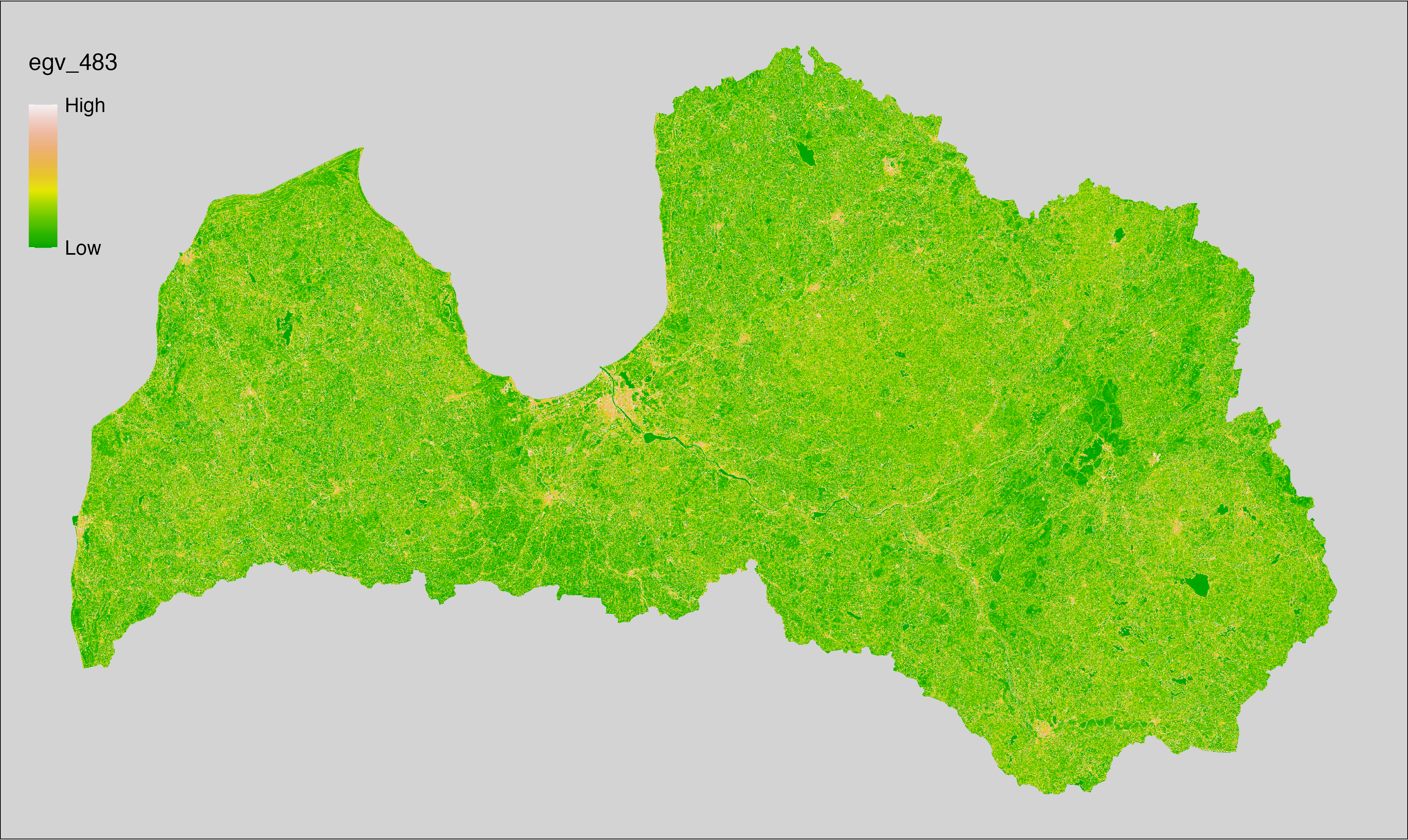
6.484 EO_NDMI-STp25-min_cell
filename: EO_NDMI-STp25-min_cell.tif
layername: egv_484
English name: Minimum short-term 25th percentile of vegetation water content index (NDMI) within the analysis cell (1 ha)
Latvian name: Minimālā 25. procentiles pēdējo gadu ūdens satura veģetācijā indeksa (NDMI) vērtība analīzes šūnā (1 ha)
Procedure: Directly follows preprocessing. The minimum value
at the analysis cell is calculated using the workflow egvtools::input2egv(). To
protect against potential data loss at edge cells, inverse distance
weighted (power = 2) gap filling is implemented. Finally, the layer is
standardised by subtracting the arithmetic mean and dividing by the root mean
squared error. The “short-term” refers to the last five years (2020-2024).
Code
# libs ----
if(!require(egvtools)) {remotes::install_github("aavotins/egvtools"); require(egvtools)}
# EO_NDMI-STp25-min_cell.tif ----
egvrez=input2egv(input="./Geodata/2024/S2indices/Mosaics/EO_NDMI-STp25.tif",
egv_template= "./Templates/TemplateRasters/LV100m_10km.tif",
summary_function = "min",
missing_job = "FillOutput",
outlocation = "./RasterGrids_100m/2024/RAW/",
outfilename = "EO_NDMI-STp25-min_cell.tif",
layername = "egv_484",
idw_weight = 2,
plot_gaps = FALSE,
plot_final = FALSE)
egvrez
# standardisation ----
if(!require(terra)) {install.packages("terra"); require(terra)}
if(!require(tidyverse)) {install.packages("tidyverse"); require(tidyverse)}
nosaukums="EO_NDMI-STp25-min_cell.tif"
ielasisanas_cels=paste0("./RasterGrids_100m/2024/RAW/",nosaukums)
saglabasanas_cels=paste0("./RasterGrids_100m/2024/Scaled/",nosaukums)
slanis=rast(ielasisanas_cels)
videjais=global(slanis,fun="mean",na.rm=TRUE)
centrets=slanis-videjais[,1]
standartnovirze=terra::global(centrets,fun="rms",na.rm=TRUE)
merogots=centrets/standartnovirze[,1]
writeRaster(merogots,
filename=saglabasanas_cels,
overwrite=TRUE)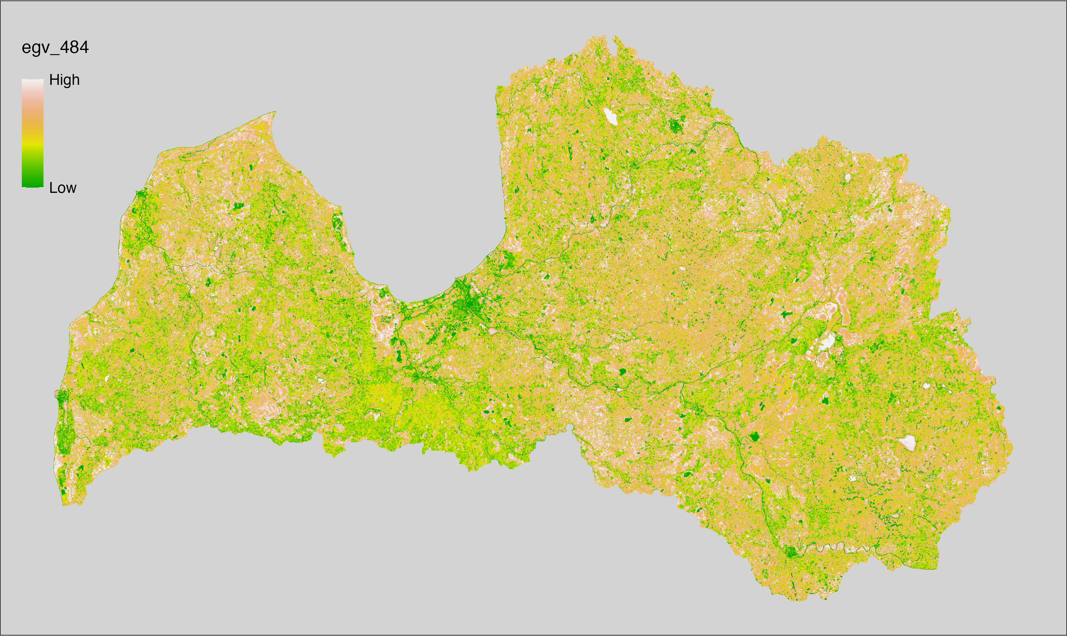
6.485 EO_NDMI-STp75-max_cell
filename: EO_NDMI-STp75-max_cell.tif
layername: egv_485
English name: Maximum short-term 75th percentile of vegetation water content index (NDMI) within the analysis cell (1 ha)
Latvian name: Maksimālā 75. procentiles pēdējo gadu ūdens satura veģetācijā indeksa (NDMI) vērtība analīzes šūnā (1 ha)
Procedure: Directly follows preprocessing. The maximum value
at the analysis cell is calculated using the workflow egvtools::input2egv(). To
protect against potential data loss at edge cells, inverse distance
weighted (power = 2) gap filling is implemented. Finally, the layer is
standardised by subtracting the arithmetic mean and dividing by the root mean
squared error. The “short-term” refers to the last five years (2020-2024).
Code
# libs ----
if(!require(egvtools)) {remotes::install_github("aavotins/egvtools"); require(egvtools)}
# EO_NDMI-STp75-max_cell.tif ----
egvrez=input2egv(input="./Geodata/2024/S2indices/Mosaics/EO_NDMI-STp75.tif",
egv_template= "./Templates/TemplateRasters/LV100m_10km.tif",
summary_function = "min",
missing_job = "FillOutput",
outlocation = "./RasterGrids_100m/2024/RAW/",
outfilename = "EO_NDMI-STp75-max_cell.tif",
layername = "egv_485",
idw_weight = 2,
plot_gaps = FALSE,
plot_final = FALSE)
egvrez
# standardisation ----
if(!require(terra)) {install.packages("terra"); require(terra)}
if(!require(tidyverse)) {install.packages("tidyverse"); require(tidyverse)}
nosaukums="EO_NDMI-STp75-max_cell.tif"
ielasisanas_cels=paste0("./RasterGrids_100m/2024/RAW/",nosaukums)
saglabasanas_cels=paste0("./RasterGrids_100m/2024/Scaled/",nosaukums)
slanis=rast(ielasisanas_cels)
videjais=global(slanis,fun="mean",na.rm=TRUE)
centrets=slanis-videjais[,1]
standartnovirze=terra::global(centrets,fun="rms",na.rm=TRUE)
merogots=centrets/standartnovirze[,1]
writeRaster(merogots,
filename=saglabasanas_cels,
overwrite=TRUE)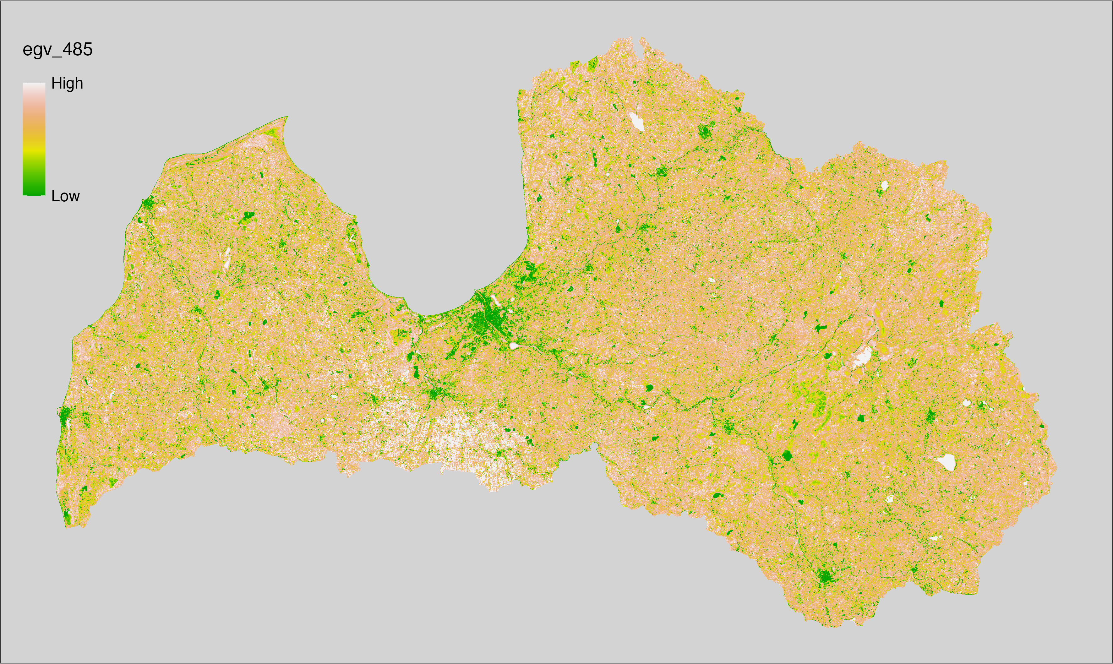
6.486 EO_NDVI-LYmedian-average_cell
filename: EO_NDVI-LYmedian-average_cell.tif
layername: egv_486
English name: Median vegetation index (NDVI) for the last year within the analysis cell (1 ha)
Latvian name: Mediānā pēdējā gada veģetācijas indeksa (NDVI) vērtība analīzes šūnā (1 ha)
Procedure: Directly follows preprocessing. The arithmetic mean value
at the analysis cell is calculated using the workflow egvtools::input2egv(). To protect against
potential data loss at edge cells, inverse distance weighted (power = 2) gap
filling is implemented. Finally, the layer is
standardised by subtracting the arithmetic mean and
dividing by the root mean squared error. The “last year” is 2024.
Code
# libs ----
if(!require(egvtools)) {remotes::install_github("aavotins/egvtools"); require(egvtools)}
# EO_NDVI-LYmedian-average_cell.tif ----
egvrez=input2egv(input="./Geodata/2024/S2indices/Mosaics/EO_NDVI-LYmedian.tif",
egv_template= "./Templates/TemplateRasters/LV100m_10km.tif",
summary_function = "average",
missing_job = "FillOutput",
outlocation = "./RasterGrids_100m/2024/RAW/",
outfilename = "EO_NDVI-LYmedian-average_cell.tif",
layername = "egv_486",
idw_weight = 2,
plot_gaps = FALSE,
plot_final = FALSE)
egvrez
# standardisation ----
if(!require(terra)) {install.packages("terra"); require(terra)}
if(!require(tidyverse)) {install.packages("tidyverse"); require(tidyverse)}
nosaukums="EO_NDVI-LYmedian-average_cell.tif"
ielasisanas_cels=paste0("./RasterGrids_100m/2024/RAW/",nosaukums)
saglabasanas_cels=paste0("./RasterGrids_100m/2024/Scaled/",nosaukums)
slanis=rast(ielasisanas_cels)
videjais=global(slanis,fun="mean",na.rm=TRUE)
centrets=slanis-videjais[,1]
standartnovirze=terra::global(centrets,fun="rms",na.rm=TRUE)
merogots=centrets/standartnovirze[,1]
writeRaster(merogots,
filename=saglabasanas_cels,
overwrite=TRUE)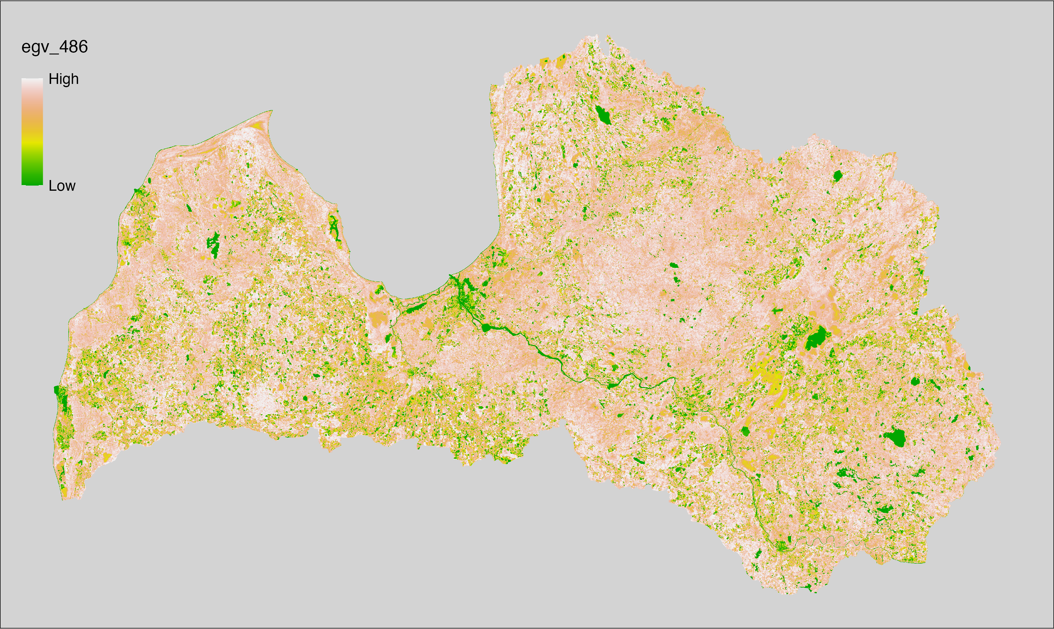
6.487 EO_NDVI-LYmedian-iqr_cell
filename: EO_NDVI-LYmedian-iqr_cell.tif
layername: egv_487
English name: Spatial variability of last year’s median vegetation index (NDVI) within the analysis cell (1 ha)
Latvian name: Telpiskā variabilitāte pēdējā gada mediānajai veģetācijas indeksa (NDVI) vērtībai analīzes šūnā (1 ha)
Procedure: Directly follows preprocessing. The
workflow egvtools::input2egv() is used to calculate Q1 and Q3 for every cell.
To protect against potential data loss at the edges, inverse distance
weighted (power = 2) gap filling is implemented. Next, Q1 is subtracted from Q3.
Finally, the layer is standardised by subtracting the arithmetic mean and
dividing by the root mean squared error. The “last year” is 2024.
Code
# libs ----
if(!require(egvtools)) {remotes::install_github("aavotins/egvtools"); require(egvtools)}
# EO_NDVI-LYmedian-iqr_cell.tif ----
p25rez=input2egv(input="./Geodata/2024/S2indices/Mosaics/EO_NDVI-LYmedian.tif",
egv_template= "./Templates/TemplateRasters/LV100m_10km.tif",
summary_function = "q1",
missing_job = "FillOutput",
outlocation = "./RasterGrids_100m/2024/",
outfilename = "draza_p25.tif",
layername = "egv_487",
idw_weight = 2,
plot_gaps = FALSE,
plot_final = FALSE)
p25rez_r=rast("./RasterGrids_100m/2024/draza_p25.tif")
p75rez=input2egv(input="./Geodata/2024/S2indices/Mosaics/EO_NDVI-LYmedian.tif",
egv_template= "./Templates/TemplateRasters/LV100m_10km.tif",
summary_function = "q3",
missing_job = "FillOutput",
outlocation = "./RasterGrids_100m/2024/",
outfilename = "draza_p75.tif",
layername = "egv_487",
idw_weight = 2,
plot_gaps = FALSE,
plot_final = FALSE)
p75rez_r=rast("./RasterGrids_100m/2024/draza_p75.tif")
iqr_rez=p75rez_r-p25rez_r
iqr_rez
plot(iqr_rez)
writeRaster(iqr_rez,
"./RasterGrids_100m/2024/RAW/EO_NDVI-LYmedian-iqr_cell.tif",
overwrite=TRUE)
unlink("./RasterGrids_100m/2024/draza_p75.tif")
unlink("./RasterGrids_100m/2024/draza_p25.tif")
# standardisation ----
if(!require(terra)) {install.packages("terra"); require(terra)}
if(!require(tidyverse)) {install.packages("tidyverse"); require(tidyverse)}
nosaukums="EO_NDVI-LYmedian-iqr_cell.tif"
ielasisanas_cels=paste0("./RasterGrids_100m/2024/RAW/",nosaukums)
saglabasanas_cels=paste0("./RasterGrids_100m/2024/Scaled/",nosaukums)
slanis=rast(ielasisanas_cels)
videjais=global(slanis,fun="mean",na.rm=TRUE)
centrets=slanis-videjais[,1]
standartnovirze=terra::global(centrets,fun="rms",na.rm=TRUE)
merogots=centrets/standartnovirze[,1]
writeRaster(merogots,
filename=saglabasanas_cels,
overwrite=TRUE)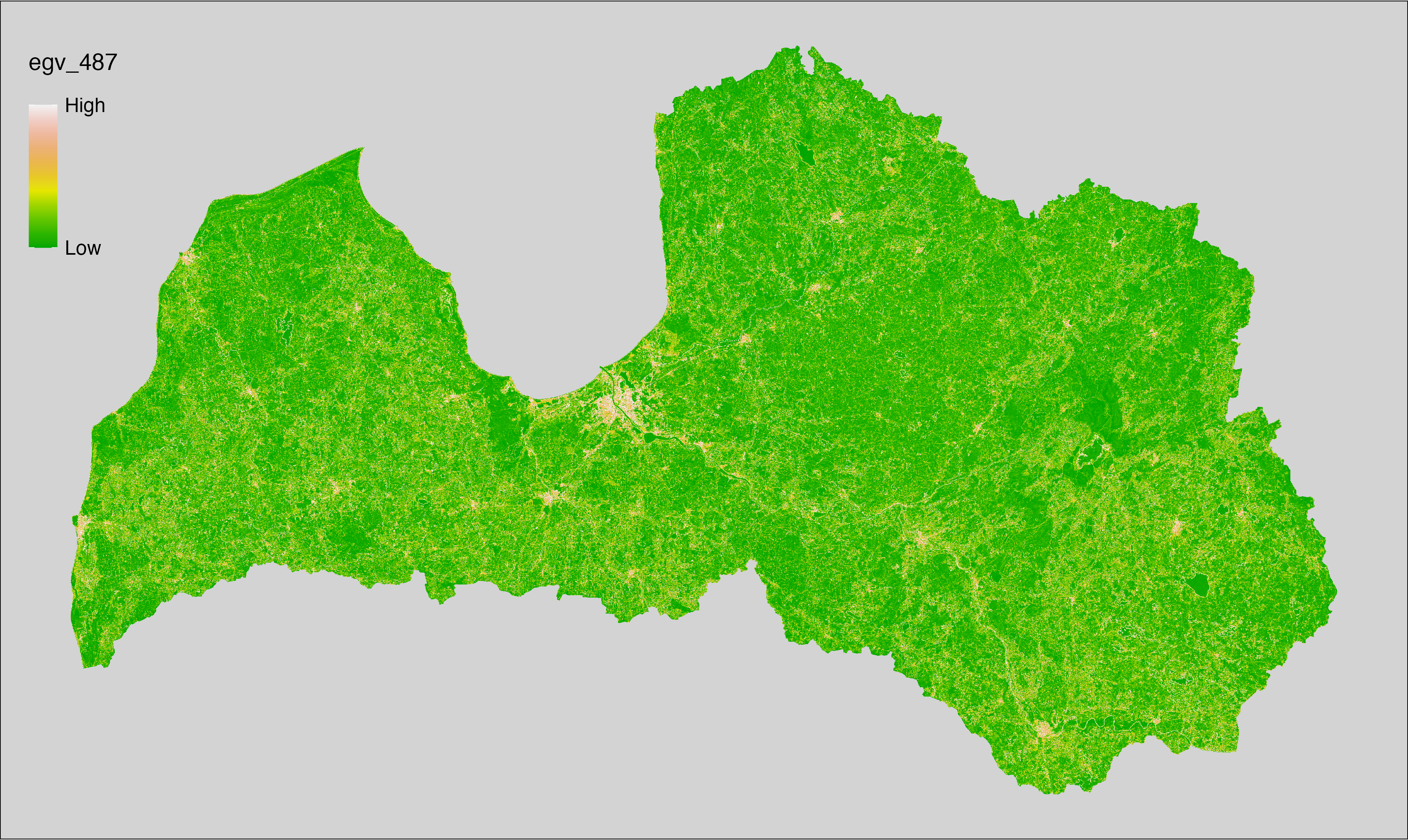
6.488 EO_NDVI-STiqr-median_cell
filename: EO_NDVI-STiqr-median_cell.tif
layername: egv_488
English name: Average short-term seasonality of vegetation index (NDVI) within the analysis cell (1 ha)
Latvian name: Sezonalitāte pēdējo gadu vidējai veģetācijas indeksa (NDVI) vērtībai analīzes šūnā (1 ha)
Procedure: Directly follows preprocessing. The arithmetic mean value
at the analysis cell is calculated using the workflow egvtools::input2egv(). To
protect against potential data loss at edge cells, inverse distance
weighted (power = 2) gap filling is implemented. Finally, the layer is
standardised by subtracting the arithmetic mean and dividing by the root mean
squared error. The “short-term” refers to the last five years (2020-2024).
Code
# libs ----
if(!require(egvtools)) {remotes::install_github("aavotins/egvtools"); require(egvtools)}
# EO_NDVI-STiqr-median_cell.tif ----
egvrez=input2egv(input="./Geodata/2024/S2indices/Mosaics/EO_NDVI-STiqr.tif",
egv_template= "./Templates/TemplateRasters/LV100m_10km.tif",
summary_function = "average",
missing_job = "FillOutput",
outlocation = "./RasterGrids_100m/2024/RAW/",
outfilename = "EO_NDVI-STiqr-median_cell.tif",
layername = "egv_488",
idw_weight = 2,
plot_gaps = FALSE,
plot_final = FALSE)
egvrez
# standardisation ----
if(!require(terra)) {install.packages("terra"); require(terra)}
if(!require(tidyverse)) {install.packages("tidyverse"); require(tidyverse)}
nosaukums="EO_NDVI-STiqr-median_cell.tif"
ielasisanas_cels=paste0("./RasterGrids_100m/2024/RAW/",nosaukums)
saglabasanas_cels=paste0("./RasterGrids_100m/2024/Scaled/",nosaukums)
slanis=rast(ielasisanas_cels)
videjais=global(slanis,fun="mean",na.rm=TRUE)
centrets=slanis-videjais[,1]
standartnovirze=terra::global(centrets,fun="rms",na.rm=TRUE)
merogots=centrets/standartnovirze[,1]
writeRaster(merogots,
filename=saglabasanas_cels,
overwrite=TRUE)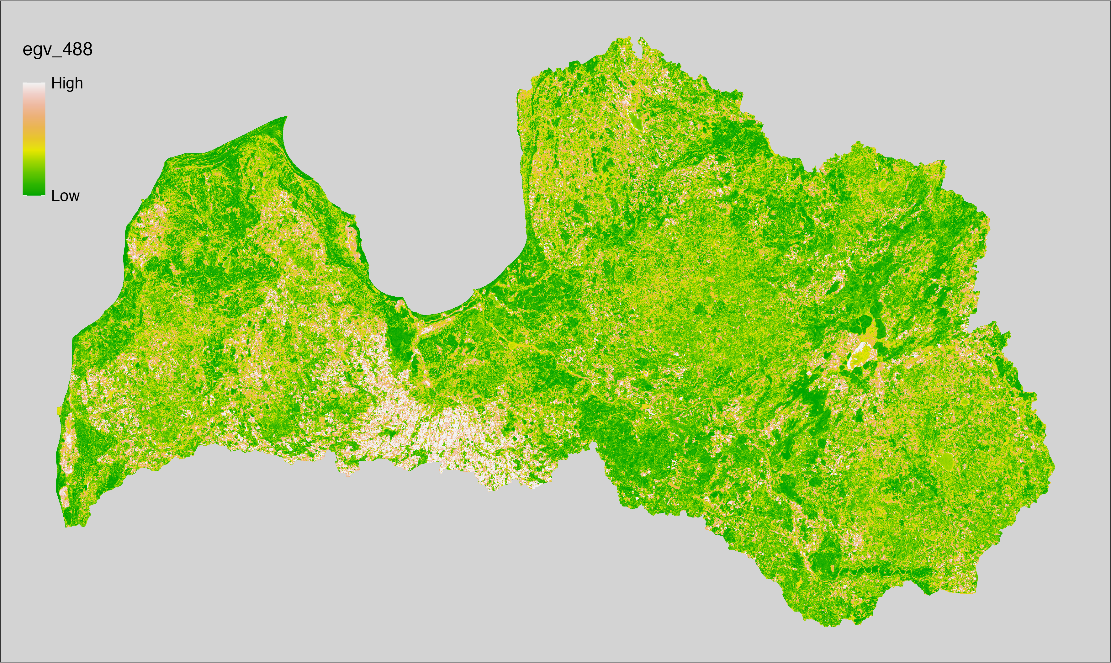
6.489 EO_NDVI-STmedian-average_cell
filename: EO_NDVI-STmedian-average_cell.tif
layername: egv_489
English name: Median short-term vegetation index (NDVI) within the analysis cell (1 ha)
Latvian name: Mediānā pēdējo gadu veģetācijas indeksa (NDVI) vērtība analīzes šūnā (1 ha)
Procedure: Directly follows preprocessing. The arithmetic mean value
at the analysis cell is calculated using the workflow egvtools::input2egv(). To
protect against potential data loss at edge cells, inverse distance
weighted (power = 2) gap filling is implemented. Finally, the layer is
standardised by subtracting the arithmetic mean and dividing by the root mean
squared error. The “short-term” refers to the last five years (2020-2024).
Code
# libs ----
if(!require(egvtools)) {remotes::install_github("aavotins/egvtools"); require(egvtools)}
# EO_NDVI-STmedian-average_cell.tif ----
egvrez=input2egv(input="./Geodata/2024/S2indices/Mosaics/EO_NDVI-STmedian.tif",
egv_template= "./Templates/TemplateRasters/LV100m_10km.tif",
summary_function = "average",
missing_job = "FillOutput",
outlocation = "./RasterGrids_100m/2024/RAW/",
outfilename = "EO_NDVI-STmedian-average_cell.tif",
layername = "egv_489",
idw_weight = 2,
plot_gaps = FALSE,
plot_final = FALSE)
egvrez
# standardisation ----
if(!require(terra)) {install.packages("terra"); require(terra)}
if(!require(tidyverse)) {install.packages("tidyverse"); require(tidyverse)}
nosaukums="EO_NDVI-STmedian-average_cell.tif"
ielasisanas_cels=paste0("./RasterGrids_100m/2024/RAW/",nosaukums)
saglabasanas_cels=paste0("./RasterGrids_100m/2024/Scaled/",nosaukums)
slanis=rast(ielasisanas_cels)
videjais=global(slanis,fun="mean",na.rm=TRUE)
centrets=slanis-videjais[,1]
standartnovirze=terra::global(centrets,fun="rms",na.rm=TRUE)
merogots=centrets/standartnovirze[,1]
writeRaster(merogots,
filename=saglabasanas_cels,
overwrite=TRUE)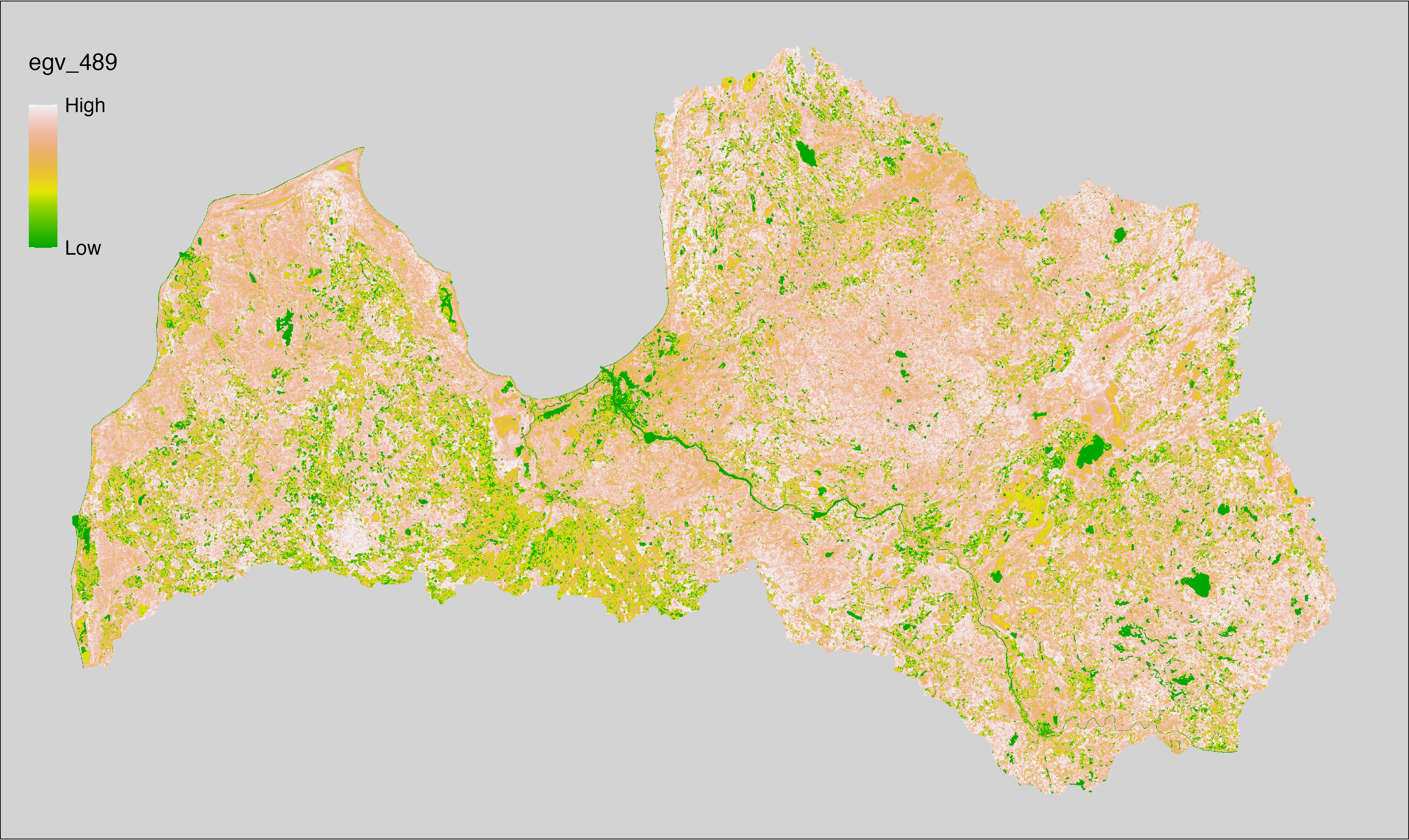
6.490 EO_NDVI-STmedian-iqr_cell
filename: EO_NDVI-STmedian-iqr_cell.tif
layername: egv_490
English name: Spatial variability of short-term median vegetation index (NDVI) within the analysis cell (1 ha)
Latvian name: Telpiskā variabilitāte pēdējo gadu mediānajai veģetācijas indeksa (NDVI) vērtībai analīzes šūnā (1 ha)
Procedure: Directly follows preprocessing. The
workflow egvtools::input2egv() is used to calculate Q1 and Q3 for every cell.
To protect against potential data loss at the edges, inverse distance
weighted (power = 2) gap filling is implemented. Next, Q1 is subtracted from Q3.
Finally, the layer is standardised by subtracting the arithmetic mean and
dividing by the root mean squared error. The “short-term” refers to the last
five years (2020-2024).
Code
# libs ----
if(!require(egvtools)) {remotes::install_github("aavotins/egvtools"); require(egvtools)}
# EO_NDVI-STmedian-iqr_cell.tif ----
p25rez=input2egv(input="./Geodata/2024/S2indices/Mosaics/EO_NDVI-STmedian.tif",
egv_template= "./Templates/TemplateRasters/LV100m_10km.tif",
summary_function = "q1",
missing_job = "FillOutput",
outlocation = "./RasterGrids_100m/2024/",
outfilename = "draza_p25.tif",
layername = "egv_490",
idw_weight = 2,
plot_gaps = FALSE,
plot_final = FALSE)
p25rez_r=rast("./RasterGrids_100m/2024/draza_p25.tif")
p75rez=input2egv(input="./Geodata/2024/S2indices/Mosaics/EO_NDVI-STmedian.tif",
egv_template= "./Templates/TemplateRasters/LV100m_10km.tif",
summary_function = "q3",
missing_job = "FillOutput",
outlocation = "./RasterGrids_100m/2024/",
outfilename = "draza_p75.tif",
layername = "egv_490",
idw_weight = 2,
plot_gaps = FALSE,
plot_final = FALSE)
p75rez_r=rast("./RasterGrids_100m/2024/draza_p75.tif")
iqr_rez=p75rez_r-p25rez_r
iqr_rez
plot(iqr_rez)
writeRaster(iqr_rez,
"./RasterGrids_100m/2024/RAW/EO_NDVI-STmedian-iqr_cell.tif",
overwrite=TRUE)
unlink("./RasterGrids_100m/2024/draza_p75.tif")
unlink("./RasterGrids_100m/2024/draza_p25.tif")
# standardisation ----
if(!require(terra)) {install.packages("terra"); require(terra)}
if(!require(tidyverse)) {install.packages("tidyverse"); require(tidyverse)}
nosaukums="EO_NDVI-STmedian-iqr_cell.tif"
ielasisanas_cels=paste0("./RasterGrids_100m/2024/RAW/",nosaukums)
saglabasanas_cels=paste0("./RasterGrids_100m/2024/Scaled/",nosaukums)
slanis=rast(ielasisanas_cels)
videjais=global(slanis,fun="mean",na.rm=TRUE)
centrets=slanis-videjais[,1]
standartnovirze=terra::global(centrets,fun="rms",na.rm=TRUE)
merogots=centrets/standartnovirze[,1]
writeRaster(merogots,
filename=saglabasanas_cels,
overwrite=TRUE)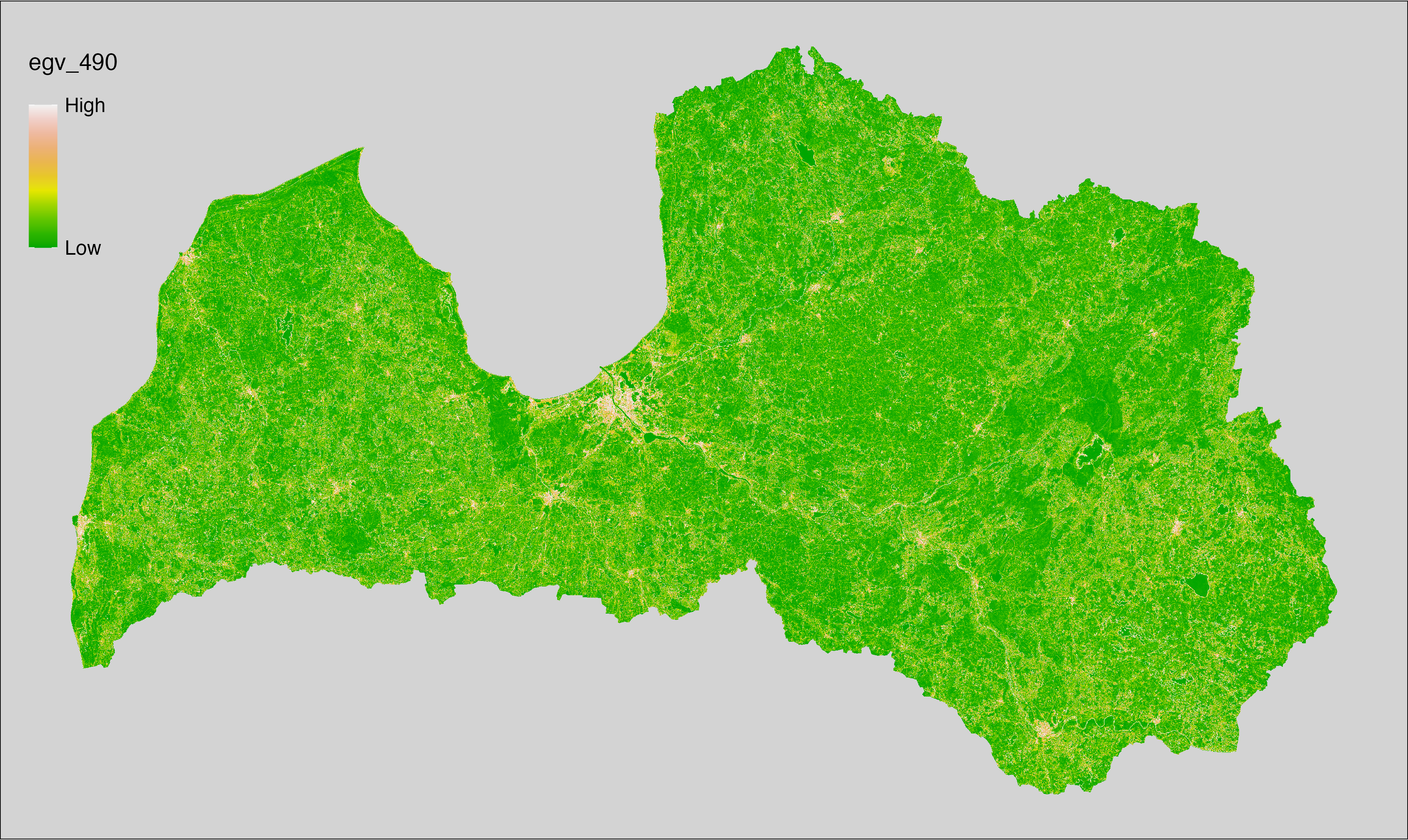
6.491 EO_NDVI-STp25-min_cell
filename: EO_NDVI-STp25-min_cell.tif
layername: egv_491
English name: Minimum short-term 25th percentile of vegetation index (NDVI) within the analysis cell (1 ha)
Latvian name: Minimālā 25. procentiles pēdējo gadu veģetācijas indeksa (NDVI) vērtība analīzes šūnā (1 ha)
Procedure: Directly follows preprocessing. The minimum value
at the analysis cell is calculated using the workflow egvtools::input2egv(). To
protect against potential data loss at edge cells, inverse distance
weighted (power = 2) gap filling is implemented. Finally, the layer is
standardised by subtracting the arithmetic mean and dividing by the root mean
squared error. The “short-term” refers to the last five years (2020-2024).
Code
# libs ----
if(!require(egvtools)) {remotes::install_github("aavotins/egvtools"); require(egvtools)}
# EO_NDVI-STp25-min_cell.tif ----
egvrez=input2egv(input="./Geodata/2024/S2indices/Mosaics/EO_NDVI-STp25.tif",
egv_template= "./Templates/TemplateRasters/LV100m_10km.tif",
summary_function = "min",
missing_job = "FillOutput",
outlocation = "./RasterGrids_100m/2024/RAW/",
outfilename = "EO_NDVI-STp25-min_cell.tif",
layername = "egv_491",
idw_weight = 2,
plot_gaps = FALSE,
plot_final = FALSE)
egvrez
# standardisation ----
if(!require(terra)) {install.packages("terra"); require(terra)}
if(!require(tidyverse)) {install.packages("tidyverse"); require(tidyverse)}
nosaukums="EO_NDVI-STp25-min_cell.tif"
ielasisanas_cels=paste0("./RasterGrids_100m/2024/RAW/",nosaukums)
saglabasanas_cels=paste0("./RasterGrids_100m/2024/Scaled/",nosaukums)
slanis=rast(ielasisanas_cels)
videjais=global(slanis,fun="mean",na.rm=TRUE)
centrets=slanis-videjais[,1]
standartnovirze=terra::global(centrets,fun="rms",na.rm=TRUE)
merogots=centrets/standartnovirze[,1]
writeRaster(merogots,
filename=saglabasanas_cels,
overwrite=TRUE)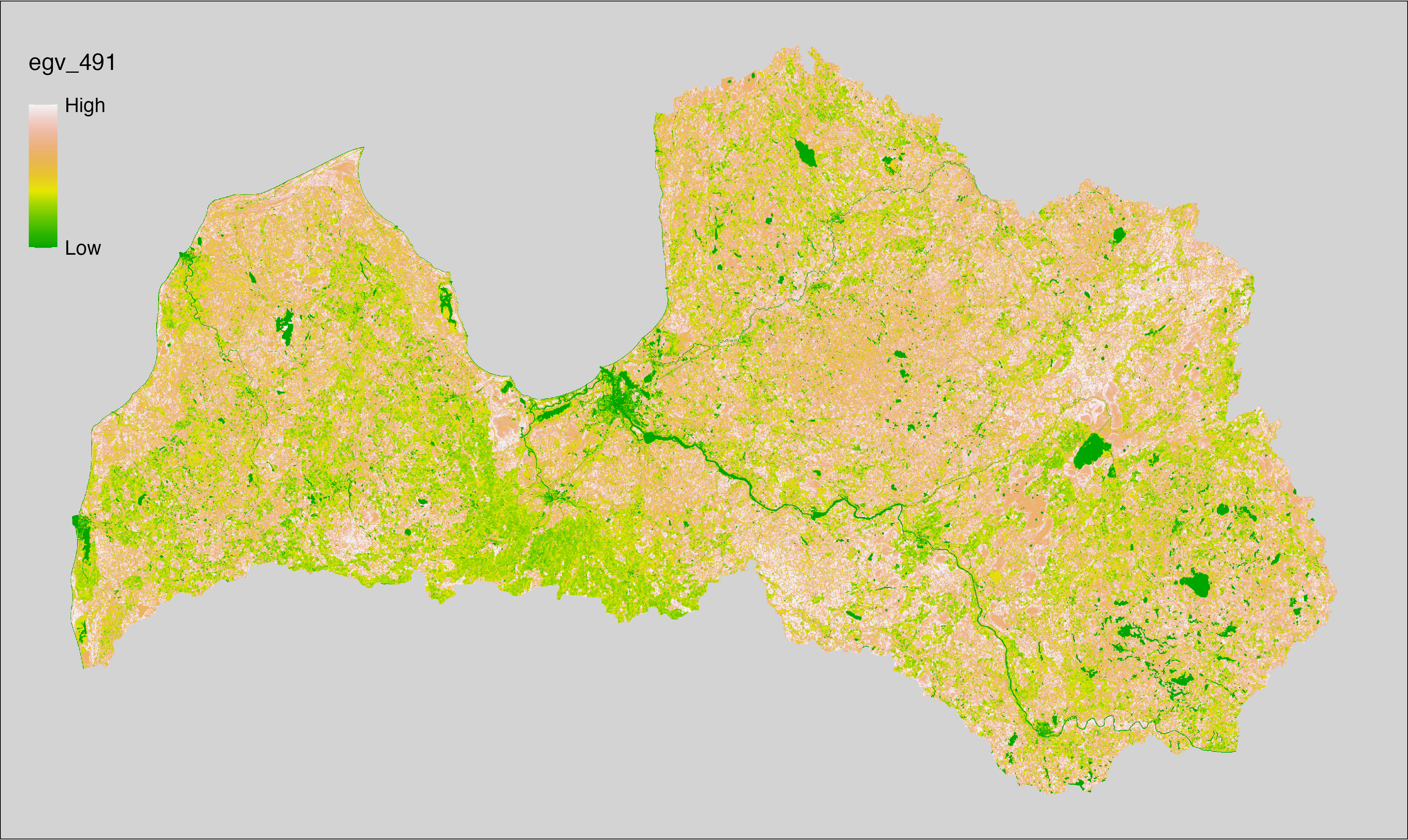
6.492 EO_NDVI-STp75-max_cell
filename: EO_NDVI-STp75-max_cell.tif
layername: egv_492
English name: Maximum short-term 75th percentile of vegetation index (NDVI) within the analysis cell (1 ha)
Latvian name: Maksimālā 75. procentiles pēdējo gadu veģetācijas indeksa (NDVI) vērtība analīzes šūnā (1 ha)
Procedure: Directly follows preprocessing. The maximum value
at the analysis cell is calculated using the workflow egvtools::input2egv(). To
protect against potential data loss at edge cells, inverse distance
weighted (power = 2) gap filling is implemented. Finally, the layer is
standardised by subtracting the arithmetic mean and dividing by the root mean
squared error. The “short-term” refers to the last five years (2020-2024).
Code
# libs ----
if(!require(egvtools)) {remotes::install_github("aavotins/egvtools"); require(egvtools)}
# EO_NDVI-STp75-max_cell.tif ----
egvrez=input2egv(input="./Geodata/2024/S2indices/Mosaics/EO_NDVI-STp75.tif",
egv_template= "./Templates/TemplateRasters/LV100m_10km.tif",
summary_function = "min",
missing_job = "FillOutput",
outlocation = "./RasterGrids_100m/2024/RAW/",
outfilename = "EO_NDVI-STp75-max_cell.tif",
layername = "egv_492",
idw_weight = 2,
plot_gaps = FALSE,
plot_final = FALSE)
egvrez
# standardisation ----
if(!require(terra)) {install.packages("terra"); require(terra)}
if(!require(tidyverse)) {install.packages("tidyverse"); require(tidyverse)}
nosaukums="EO_NDVI-STp75-max_cell.tif"
ielasisanas_cels=paste0("./RasterGrids_100m/2024/RAW/",nosaukums)
saglabasanas_cels=paste0("./RasterGrids_100m/2024/Scaled/",nosaukums)
slanis=rast(ielasisanas_cels)
videjais=global(slanis,fun="mean",na.rm=TRUE)
centrets=slanis-videjais[,1]
standartnovirze=terra::global(centrets,fun="rms",na.rm=TRUE)
merogots=centrets/standartnovirze[,1]
writeRaster(merogots,
filename=saglabasanas_cels,
overwrite=TRUE)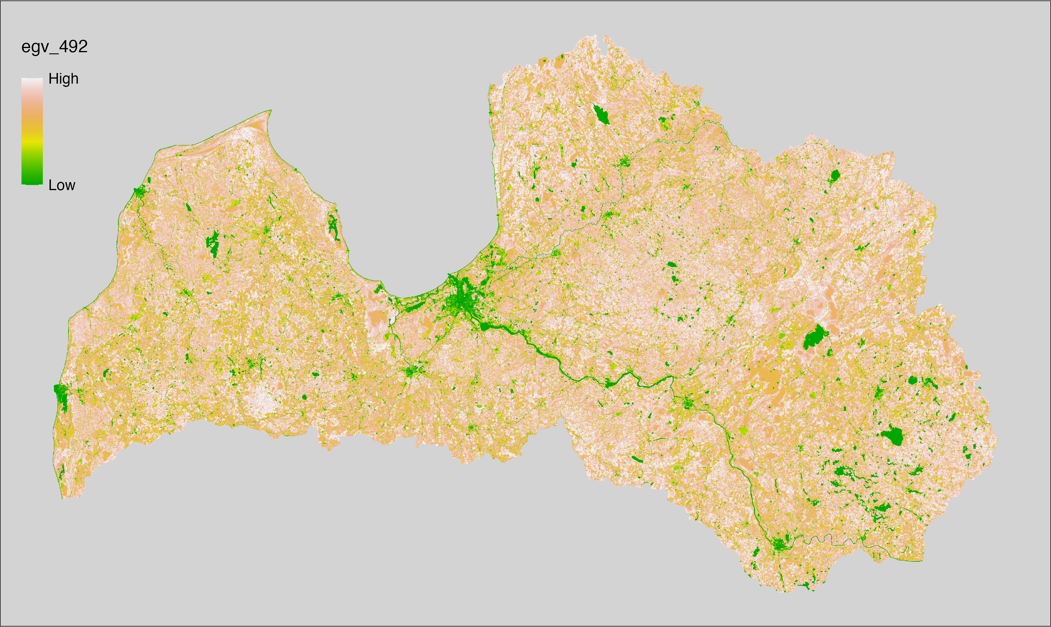
6.493 EO_NDWI-LYmedian-average_cell
filename: EO_NDWI-LYmedian-average_cell.tif
layername: egv_493
English name: Median water index (NDWI) for the last year within the analysis cell (1 ha)
Latvian name: Mediānā pēdējā gada ūdens indeksa (NDWI) vērtība analīzes šūnā (1 ha)
Procedure: Directly follows preprocessing. The arithmetic mean value
at the analysis cell is calculated using the workflow egvtools::input2egv(). To protect against
potential data loss at edge cells, inverse distance weighted (power = 2) gap
filling is implemented. Finally, the layer is
standardised by subtracting the arithmetic mean and
dividing by the root mean squared error. The “last year” is 2024.
Code
# libs ----
if(!require(egvtools)) {remotes::install_github("aavotins/egvtools"); require(egvtools)}
egvrez=input2egv(input="./Geodata/2024/S2indices/Mosaics/EO_NDWI-LYmedian.tif",
egv_template= "./Templates/TemplateRasters/LV100m_10km.tif",
summary_function = "average",
missing_job = "FillOutput",
outlocation = "./RasterGrids_100m/2024/RAW/",
outfilename = "EO_NDWI-LYmedian-average_cell.tif",
layername = "egv_493",
idw_weight = 2,
plot_gaps = FALSE,
plot_final = FALSE)
egvrez
# standardisation ----
if(!require(terra)) {install.packages("terra"); require(terra)}
if(!require(tidyverse)) {install.packages("tidyverse"); require(tidyverse)}
nosaukums="EO_NDWI-LYmedian-average_cell.tif"
ielasisanas_cels=paste0("./RasterGrids_100m/2024/RAW/",nosaukums)
saglabasanas_cels=paste0("./RasterGrids_100m/2024/Scaled/",nosaukums)
slanis=rast(ielasisanas_cels)
videjais=global(slanis,fun="mean",na.rm=TRUE)
centrets=slanis-videjais[,1]
standartnovirze=terra::global(centrets,fun="rms",na.rm=TRUE)
merogots=centrets/standartnovirze[,1]
writeRaster(merogots,
filename=saglabasanas_cels,
overwrite=TRUE)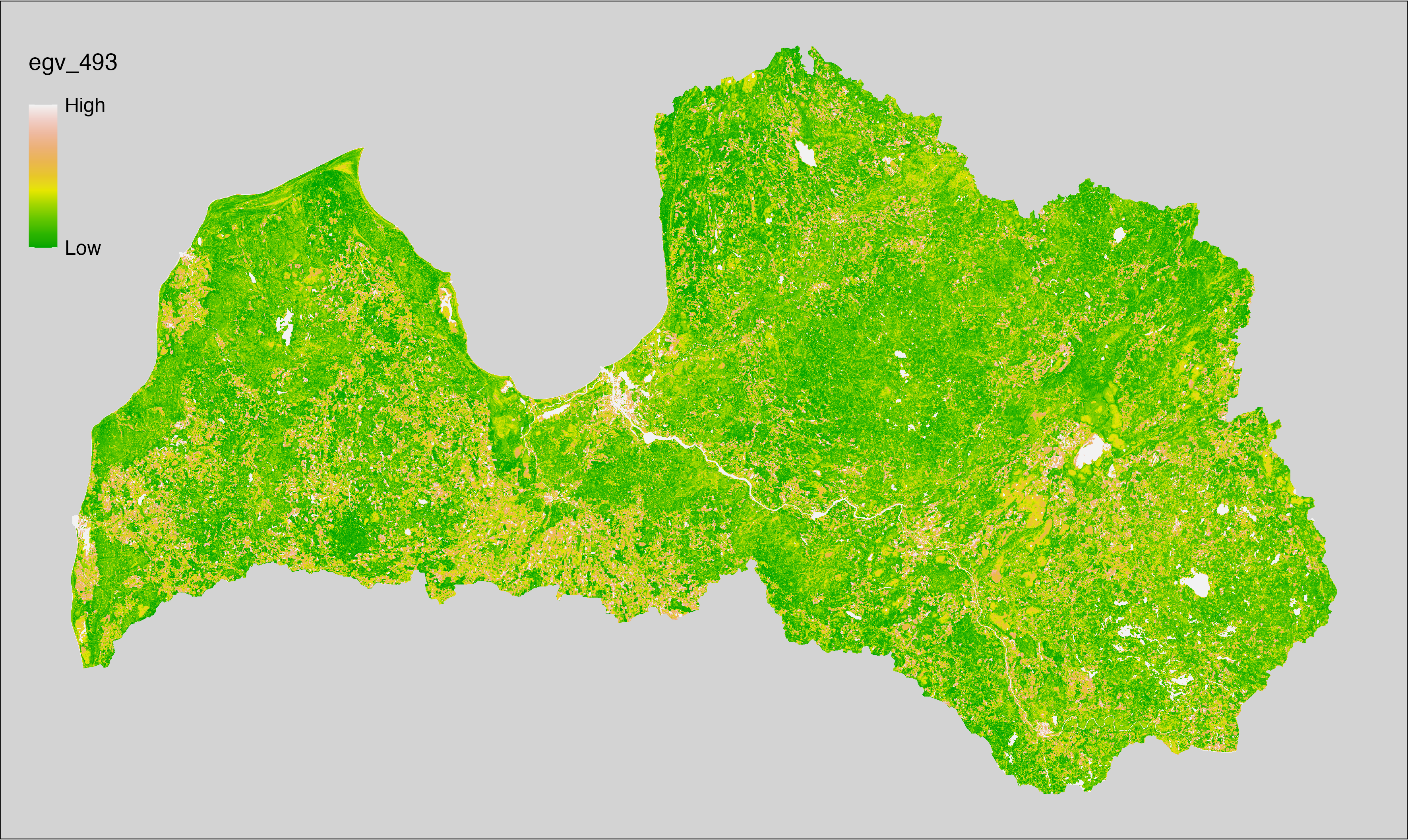
6.494 EO_NDWI-LYmedian-iqr_cell
filename: EO_NDWI-LYmedian-iqr_cell.tif
layername: egv_494
English name: Spatial variability of last year’s median water index (NDWI) within the analysis cell (1 ha)
Latvian name: Telpiskā variabilitāte pēdējā gada mediānajai ūdens indeksa (NDWI) vērtībai analīzes šūnā (1 ha)
Procedure: Directly follows preprocessing. The
workflow egvtools::input2egv() is used to calculate Q1 and Q3 for every cell.
To protect against potential data loss at the edges, inverse distance
weighted (power = 2) gap filling is implemented. Next, Q1 is subtracted from Q3.
Finally, the layer is standardised by subtracting the arithmetic mean and
dividing by the root mean squared error. The “last year” is 2024.
Code
# libs ----
if(!require(egvtools)) {remotes::install_github("aavotins/egvtools"); require(egvtools)}
# EO_NDWI-LYmedian-iqr_cell.tif ----
p25rez=input2egv(input="./Geodata/2024/S2indices/Mosaics/EO_NDWI-LYmedian.tif",
egv_template= "./Templates/TemplateRasters/LV100m_10km.tif",
summary_function = "q1",
missing_job = "FillOutput",
outlocation = "./RasterGrids_100m/2024/",
outfilename = "draza_p25.tif",
layername = "egv_494",
idw_weight = 2,
plot_gaps = FALSE,
plot_final = FALSE)
p25rez_r=rast("./RasterGrids_100m/2024/draza_p25.tif")
p75rez=input2egv(input="./Geodata/2024/S2indices/Mosaics/EO_NDWI-LYmedian.tif",
egv_template= "./Templates/TemplateRasters/LV100m_10km.tif",
summary_function = "q3",
missing_job = "FillOutput",
outlocation = "./RasterGrids_100m/2024/",
outfilename = "draza_p75.tif",
layername = "egv_494",
idw_weight = 2,
plot_gaps = FALSE,
plot_final = FALSE)
p75rez_r=rast("./RasterGrids_100m/2024/draza_p75.tif")
iqr_rez=p75rez_r-p25rez_r
iqr_rez
plot(iqr_rez)
writeRaster(iqr_rez,
"./RasterGrids_100m/2024/RAW/EO_NDWI-LYmedian-iqr_cell.tif",
overwrite=TRUE)
unlink("./RasterGrids_100m/2024/draza_p75.tif")
unlink("./RasterGrids_100m/2024/draza_p25.tif")
# standardisation ----
if(!require(terra)) {install.packages("terra"); require(terra)}
if(!require(tidyverse)) {install.packages("tidyverse"); require(tidyverse)}
nosaukums="EO_NDWI-LYmedian-iqr_cell.tif"
ielasisanas_cels=paste0("./RasterGrids_100m/2024/RAW/",nosaukums)
saglabasanas_cels=paste0("./RasterGrids_100m/2024/Scaled/",nosaukums)
slanis=rast(ielasisanas_cels)
videjais=global(slanis,fun="mean",na.rm=TRUE)
centrets=slanis-videjais[,1]
standartnovirze=terra::global(centrets,fun="rms",na.rm=TRUE)
merogots=centrets/standartnovirze[,1]
writeRaster(merogots,
filename=saglabasanas_cels,
overwrite=TRUE)
6.495 EO_NDWI-STiqr-median_cell
filename: EO_NDWI-STiqr-median_cell.tif
layername: egv_495
English name: Average short-term seasonality of water index (NDWI) within the analysis cell (1 ha)
Latvian name: Sezonalitāte pēdējo gadu vidējai ūdens indeksa (NDWI) vērtībai analīzes šūnā (1 ha)
Procedure: Directly follows preprocessing. The arithmetic mean value
at the analysis cell is calculated using the workflow egvtools::input2egv(). To
protect against potential data loss at edge cells, inverse distance
weighted (power = 2) gap filling is implemented. Finally, the layer is
standardised by subtracting the arithmetic mean and dividing by the root mean
squared error. The “short-term” refers to the last five years (2020-2024).
Code
# libs ----
if(!require(egvtools)) {remotes::install_github("aavotins/egvtools"); require(egvtools)}
# EO_NDWI-STiqr-median_cell.tif ----
egvrez=input2egv(input="./Geodata/2024/S2indices/Mosaics/EO_NDWI-STiqr.tif",
egv_template= "./Templates/TemplateRasters/LV100m_10km.tif",
summary_function = "average",
missing_job = "FillOutput",
outlocation = "./RasterGrids_100m/2024/RAW/",
outfilename = "EO_NDWI-STiqr-median_cell.tif",
layername = "egv_495",
idw_weight = 2,
plot_gaps = FALSE,
plot_final = FALSE)
egvrez
# standardisation ----
if(!require(terra)) {install.packages("terra"); require(terra)}
if(!require(tidyverse)) {install.packages("tidyverse"); require(tidyverse)}
nosaukums="EO_NDWI-STiqr-median_cell.tif"
ielasisanas_cels=paste0("./RasterGrids_100m/2024/RAW/",nosaukums)
saglabasanas_cels=paste0("./RasterGrids_100m/2024/Scaled/",nosaukums)
slanis=rast(ielasisanas_cels)
videjais=global(slanis,fun="mean",na.rm=TRUE)
centrets=slanis-videjais[,1]
standartnovirze=terra::global(centrets,fun="rms",na.rm=TRUE)
merogots=centrets/standartnovirze[,1]
writeRaster(merogots,
filename=saglabasanas_cels,
overwrite=TRUE)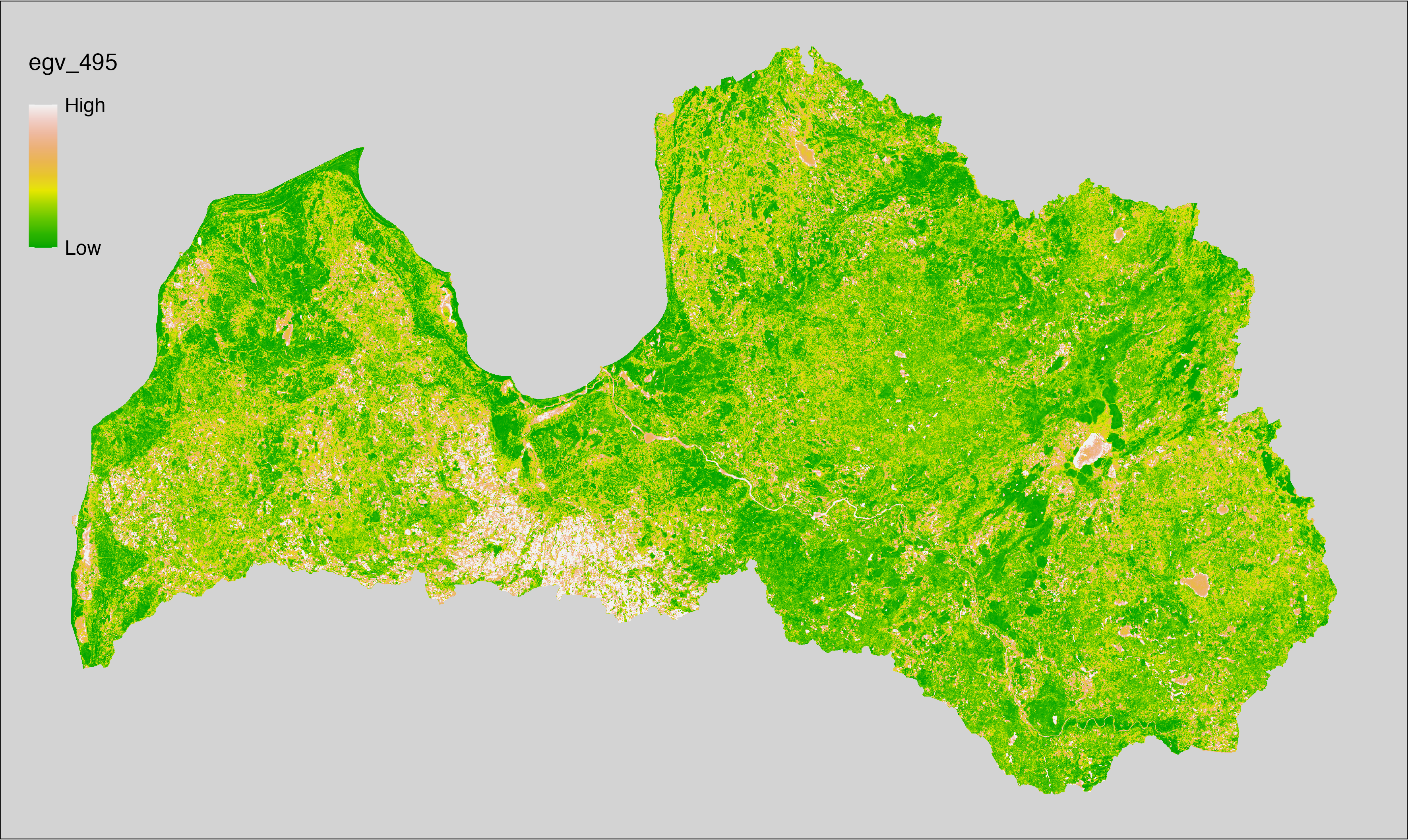
6.496 EO_NDWI-STmedian-average_cell
filename: EO_NDWI-STmedian-average_cell.tif
layername: egv_496
English name: Median short-term water index (NDWI) within the analysis cell (1 ha)
Latvian name: Mediānā pēdējo gadu ūdens indeksa (NDWI) vērtība analīzes šūnā (1 ha)
Procedure: Directly follows preprocessing. The arithmetic mean value
at the analysis cell is calculated using the workflow egvtools::input2egv(). To
protect against potential data loss at edge cells, inverse distance
weighted (power = 2) gap filling is implemented. Finally, the layer is
standardised by subtracting the arithmetic mean and dividing by the root mean
squared error. The “short-term” refers to the last five years (2020-2024).
Code
# libs ----
if(!require(egvtools)) {remotes::install_github("aavotins/egvtools"); require(egvtools)}
# EO_NDWI-STmedian-average_cell.tif ----
egvrez=input2egv(input="./Geodata/2024/S2indices/Mosaics/EO_NDWI-STmedian.tif",
egv_template= "./Templates/TemplateRasters/LV100m_10km.tif",
summary_function = "average",
missing_job = "FillOutput",
outlocation = "./RasterGrids_100m/2024/RAW/",
outfilename = "EO_NDWI-STmedian-average_cell.tif",
layername = "egv_496",
idw_weight = 2,
plot_gaps = FALSE,
plot_final = FALSE)
egvrez
# standardisation ----
if(!require(terra)) {install.packages("terra"); require(terra)}
if(!require(tidyverse)) {install.packages("tidyverse"); require(tidyverse)}
nosaukums="EO_NDWI-STmedian-average_cell.tif"
ielasisanas_cels=paste0("./RasterGrids_100m/2024/RAW/",nosaukums)
saglabasanas_cels=paste0("./RasterGrids_100m/2024/Scaled/",nosaukums)
slanis=rast(ielasisanas_cels)
videjais=global(slanis,fun="mean",na.rm=TRUE)
centrets=slanis-videjais[,1]
standartnovirze=terra::global(centrets,fun="rms",na.rm=TRUE)
merogots=centrets/standartnovirze[,1]
writeRaster(merogots,
filename=saglabasanas_cels,
overwrite=TRUE)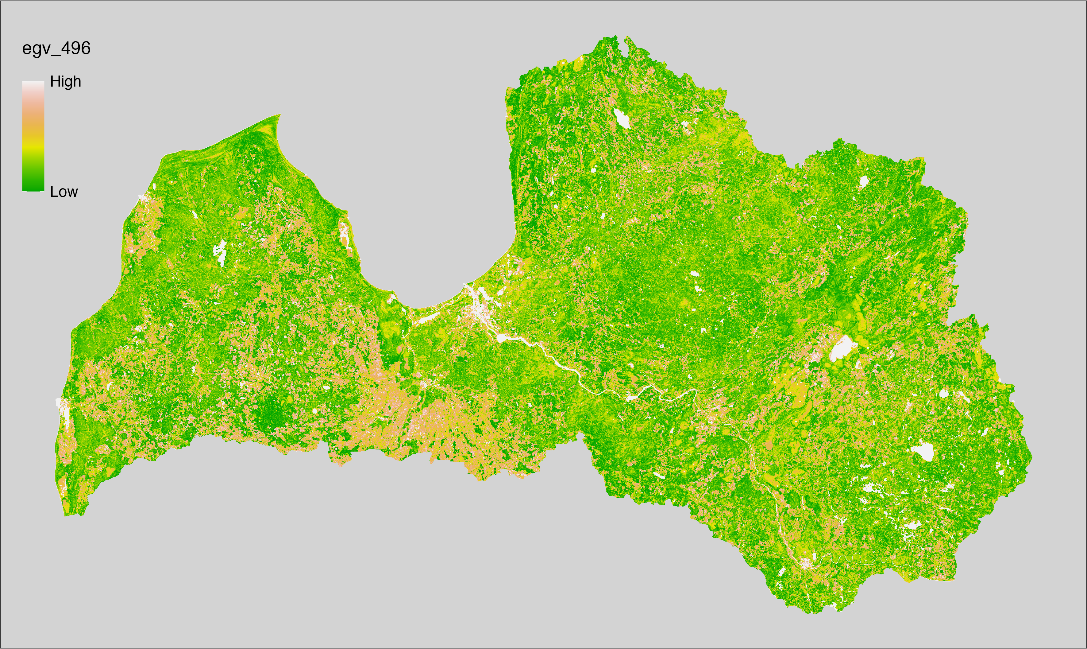
6.497 EO_NDWI-STmedian-iqr_cell
filename: EO_NDWI-STmedian-iqr_cell.tif
layername: egv_497
English name: Spatial variability of short-term median water index (NDWI) within the analysis cell (1 ha)
Latvian name: Telpiskā variabilitāte pēdējo gadu mediānajai ūdens indeksa (NDWI) vērtībai analīzes šūnā (1 ha)
Procedure: Directly follows preprocessing. The
workflow egvtools::input2egv() is used to calculate Q1 and Q3 for every cell.
To protect against potential data loss at the edges, inverse distance
weighted (power = 2) gap filling is implemented. Next, Q1 is subtracted from Q3.
Finally, the layer is standardised by subtracting the arithmetic mean and
dividing by the root mean squared error. The “short-term” refers to the last
five years (2020-2024).
Code
# libs ----
if(!require(egvtools)) {remotes::install_github("aavotins/egvtools"); require(egvtools)}
# EO_NDWI-STmedian-iqr_cell.tif ----
p25rez=input2egv(input="./Geodata/2024/S2indices/Mosaics/EO_NDWI-STmedian.tif",
egv_template= "./Templates/TemplateRasters/LV100m_10km.tif",
summary_function = "q1",
missing_job = "FillOutput",
outlocation = "./RasterGrids_100m/2024/",
outfilename = "draza_p25.tif",
layername = "egv_497",
idw_weight = 2,
plot_gaps = FALSE,
plot_final = FALSE)
p25rez_r=rast("./RasterGrids_100m/2024/draza_p25.tif")
p75rez=input2egv(input="./Geodata/2024/S2indices/Mosaics/EO_NDWI-STmedian.tif",
egv_template= "./Templates/TemplateRasters/LV100m_10km.tif",
summary_function = "q3",
missing_job = "FillOutput",
outlocation = "./RasterGrids_100m/2024/",
outfilename = "draza_p75.tif",
layername = "egv_497",
idw_weight = 2,
plot_gaps = FALSE,
plot_final = FALSE)
p75rez_r=rast("./RasterGrids_100m/2024/draza_p75.tif")
iqr_rez=p75rez_r-p25rez_r
iqr_rez
plot(iqr_rez)
writeRaster(iqr_rez,
"./RasterGrids_100m/2024/RAW/EO_NDWI-STmedian-iqr_cell.tif",
overwrite=TRUE)
unlink("./RasterGrids_100m/2024/draza_p75.tif")
unlink("./RasterGrids_100m/2024/draza_p25.tif")
# standardisation ----
if(!require(terra)) {install.packages("terra"); require(terra)}
if(!require(tidyverse)) {install.packages("tidyverse"); require(tidyverse)}
nosaukums="EO_NDWI-STmedian-iqr_cell.tif"
ielasisanas_cels=paste0("./RasterGrids_100m/2024/RAW/",nosaukums)
saglabasanas_cels=paste0("./RasterGrids_100m/2024/Scaled/",nosaukums)
slanis=rast(ielasisanas_cels)
videjais=global(slanis,fun="mean",na.rm=TRUE)
centrets=slanis-videjais[,1]
standartnovirze=terra::global(centrets,fun="rms",na.rm=TRUE)
merogots=centrets/standartnovirze[,1]
writeRaster(merogots,
filename=saglabasanas_cels,
overwrite=TRUE)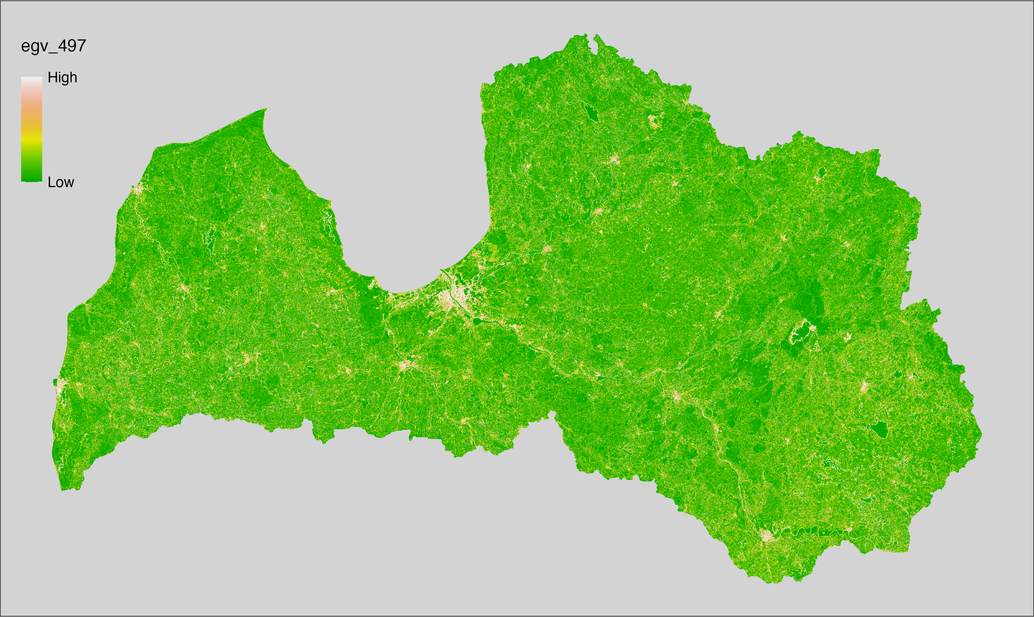
6.498 EO_NDWI-STp25-min_cell
filename: EO_NDWI-STp25-min_cell.tif
layername: egv_498
English name: Minimum short-term 25th percentile of water index (NDWI) within the analysis cell (1 ha)
Latvian name: Minimālā 25. procentiles pēdējo gadu ūdens indeksa (NDWI) vērtība analīzes šūnā (1 ha)
Procedure: Directly follows preprocessing. The minimum value
at the analysis cell is calculated using the workflow egvtools::input2egv(). To
protect against potential data loss at edge cells, inverse distance
weighted (power = 2) gap filling is implemented. Finally, the layer is
standardised by subtracting the arithmetic mean and dividing by the root mean
squared error. The “short-term” refers to the last five years (2020-2024).
Code
# libs ----
if(!require(egvtools)) {remotes::install_github("aavotins/egvtools"); require(egvtools)}
# EO_NDWI-STp25-min_cell.tif ----
egvrez=input2egv(input="./Geodata/2024/S2indices/Mosaics/EO_NDWI-STp25.tif",
egv_template= "./Templates/TemplateRasters/LV100m_10km.tif",
summary_function = "min",
missing_job = "FillOutput",
outlocation = "./RasterGrids_100m/2024/RAW/",
outfilename = "EO_NDWI-STp25-min_cell.tif",
layername = "egv_498",
idw_weight = 2,
plot_gaps = FALSE,
plot_final = FALSE)
egvrez
# standardisation ----
if(!require(terra)) {install.packages("terra"); require(terra)}
if(!require(tidyverse)) {install.packages("tidyverse"); require(tidyverse)}
nosaukums="EO_NDWI-STp25-min_cell.tif"
ielasisanas_cels=paste0("./RasterGrids_100m/2024/RAW/",nosaukums)
saglabasanas_cels=paste0("./RasterGrids_100m/2024/Scaled/",nosaukums)
slanis=rast(ielasisanas_cels)
videjais=global(slanis,fun="mean",na.rm=TRUE)
centrets=slanis-videjais[,1]
standartnovirze=terra::global(centrets,fun="rms",na.rm=TRUE)
merogots=centrets/standartnovirze[,1]
writeRaster(merogots,
filename=saglabasanas_cels,
overwrite=TRUE)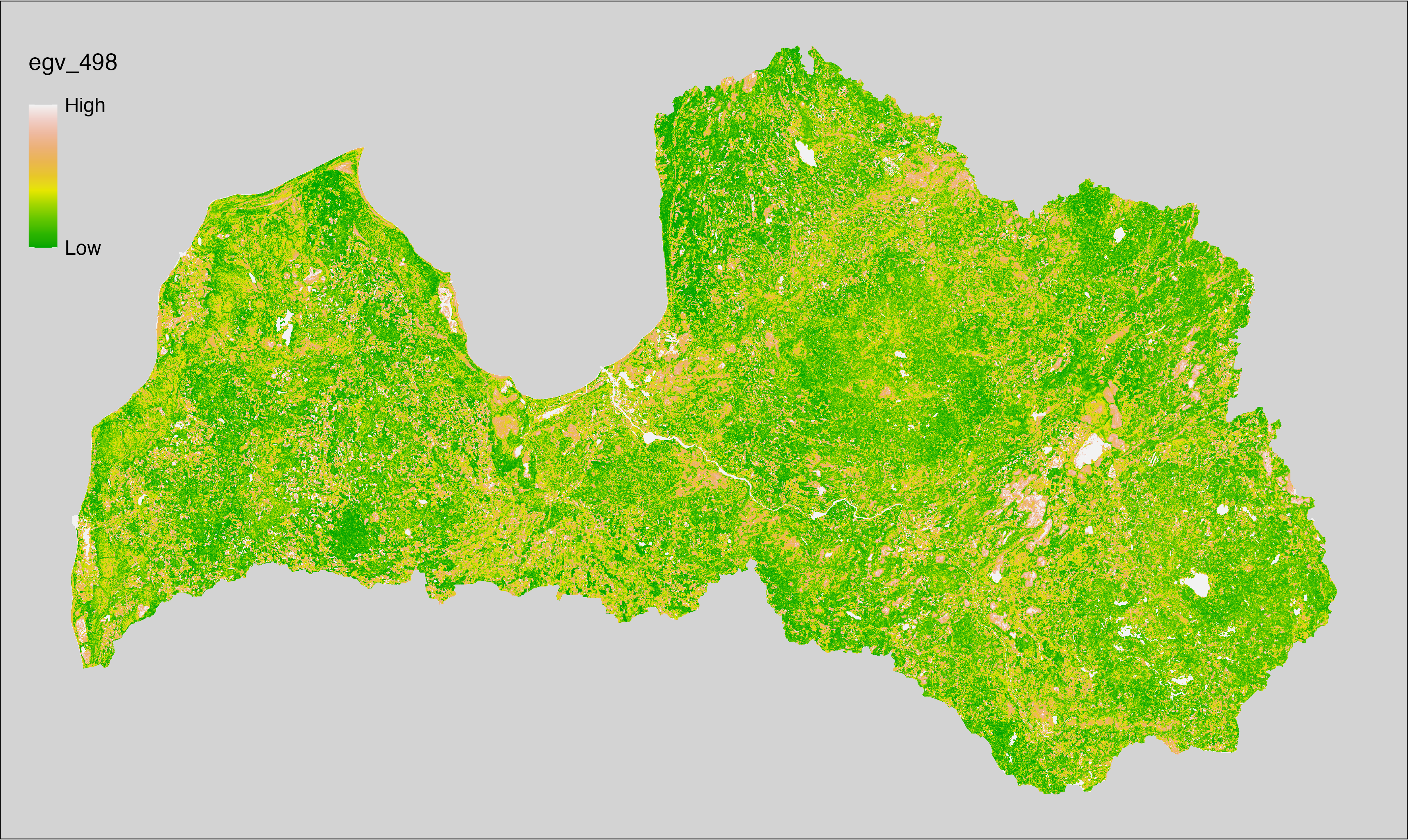
6.499 EO_NDWI-STp75-max_cell
filename: EO_NDWI-STp75-max_cell.tif
layername: egv_499
English name: Maximum short-term 75th percentile of water index (NDWI) within the analysis cell (1 ha)
Latvian name: Maksimālā 75. procentiles pēdējo gadu ūdens indeksa (NDWI) vērtība analīzes šūnā (1 ha)
Procedure: Directly follows preprocessing. The maximum value
at the analysis cell is calculated using the workflow egvtools::input2egv(). To
protect against potential data loss at edge cells, inverse distance
weighted (power = 2) gap filling is implemented. Finally, the layer is
standardised by subtracting the arithmetic mean and dividing by the root mean
squared error. The “short-term” refers to the last five years (2020-2024).
Code
# libs ----
if(!require(egvtools)) {remotes::install_github("aavotins/egvtools"); require(egvtools)}
# EO_NDWI-STp75-max_cell.tif ----
egvrez=input2egv(input="./Geodata/2024/S2indices/Mosaics/EO_NDWI-STp75.tif",
egv_template= "./Templates/TemplateRasters/LV100m_10km.tif",
summary_function = "min",
missing_job = "FillOutput",
outlocation = "./RasterGrids_100m/2024/RAW/",
outfilename = "EO_NDWI-STp75-max_cell.tif",
layername = "egv_499",
idw_weight = 2,
plot_gaps = FALSE,
plot_final = FALSE)
egvrez
# standardisation ----
if(!require(terra)) {install.packages("terra"); require(terra)}
if(!require(tidyverse)) {install.packages("tidyverse"); require(tidyverse)}
nosaukums="EO_NDWI-STp75-max_cell.tif"
ielasisanas_cels=paste0("./RasterGrids_100m/2024/RAW/",nosaukums)
saglabasanas_cels=paste0("./RasterGrids_100m/2024/Scaled/",nosaukums)
slanis=rast(ielasisanas_cels)
videjais=global(slanis,fun="mean",na.rm=TRUE)
centrets=slanis-videjais[,1]
standartnovirze=terra::global(centrets,fun="rms",na.rm=TRUE)
merogots=centrets/standartnovirze[,1]
writeRaster(merogots,
filename=saglabasanas_cels,
overwrite=TRUE)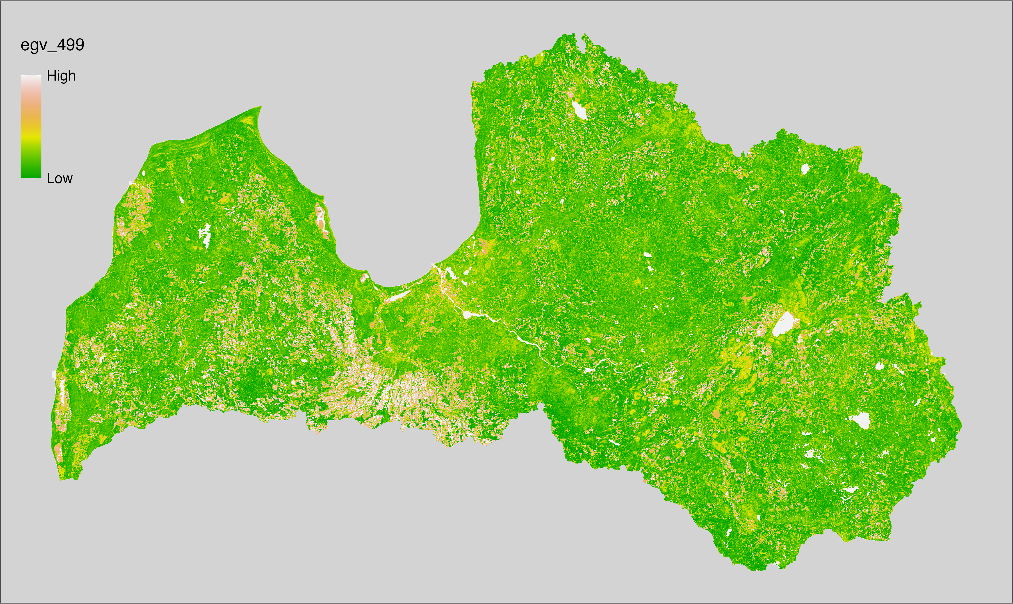
6.500 SoilChemistry_ESDAC-CN_cell
filename: SoilChemistry_ESDAC-CN_cell.tif
layername: egv_500
English name: Average value of Topsoil Carbon-Nitrogen ratio (ESDAC v2.0) within the analysis cell (1 ha)
Latvian name: Augsnes virskārtas oglekļa-slāpekļa attiecība (ESDAC v2.0) analīzes šūnā (1 ha)
Procedure: Directly derived from the Soil chemistry. Processed
using the workflow egvtools::downscale2egv() with fill gaps = TRUE, performing
inverse distance weighted (power = 2) filling of gaps at the border
and smooth = FALSE. This is done to preserve the original values as much as
possible (bilinear interpolation is involved when projecting from a 500 m
resolution to a 100 m resolution in a different CRS). Finally, the layer is
standardised by subtracting the arithmetic mean and dividing by the root mean
squared error.
Code
# libs ----
if(!require(egvtools)) {remotes::install_github("aavotins/egvtools"); require(egvtools)}
# CN ----
egv=downscale2egv(
template_path = "./Templates/TemplateRasters/LV100m_10km.tif",
grid_path = "./Templates/TemplateGrids/tikls1km_sauzeme.parquet",
rawfile_path = "./Geodata/2024/Soils/ESDAC/chemistry/chemistry/CN/CN.tif",
out_path = "./RasterGrids_100m/2024/RAW/",
file_name = "SoilChemistry_ESDAC-CN_cell.tif",
layer_name = "egv_500",
fill_gaps = TRUE,
smooth = FALSE,
plot_result = TRUE)
egv
# standardisation ----
if(!require(terra)) {install.packages("terra"); require(terra)}
if(!require(tidyverse)) {install.packages("tidyverse"); require(tidyverse)}
nosaukums="SoilChemistry_ESDAC-CN_cell.tif"
ielasisanas_cels=paste0("./RasterGrids_100m/2024/RAW/",nosaukums)
saglabasanas_cels=paste0("./RasterGrids_100m/2024/Scaled/",nosaukums)
slanis=rast(ielasisanas_cels)
videjais=global(slanis,fun="mean",na.rm=TRUE)
centrets=slanis-videjais[,1]
standartnovirze=terra::global(centrets,fun="rms",na.rm=TRUE)
merogots=centrets/standartnovirze[,1]
writeRaster(merogots,
filename=saglabasanas_cels,
overwrite=TRUE)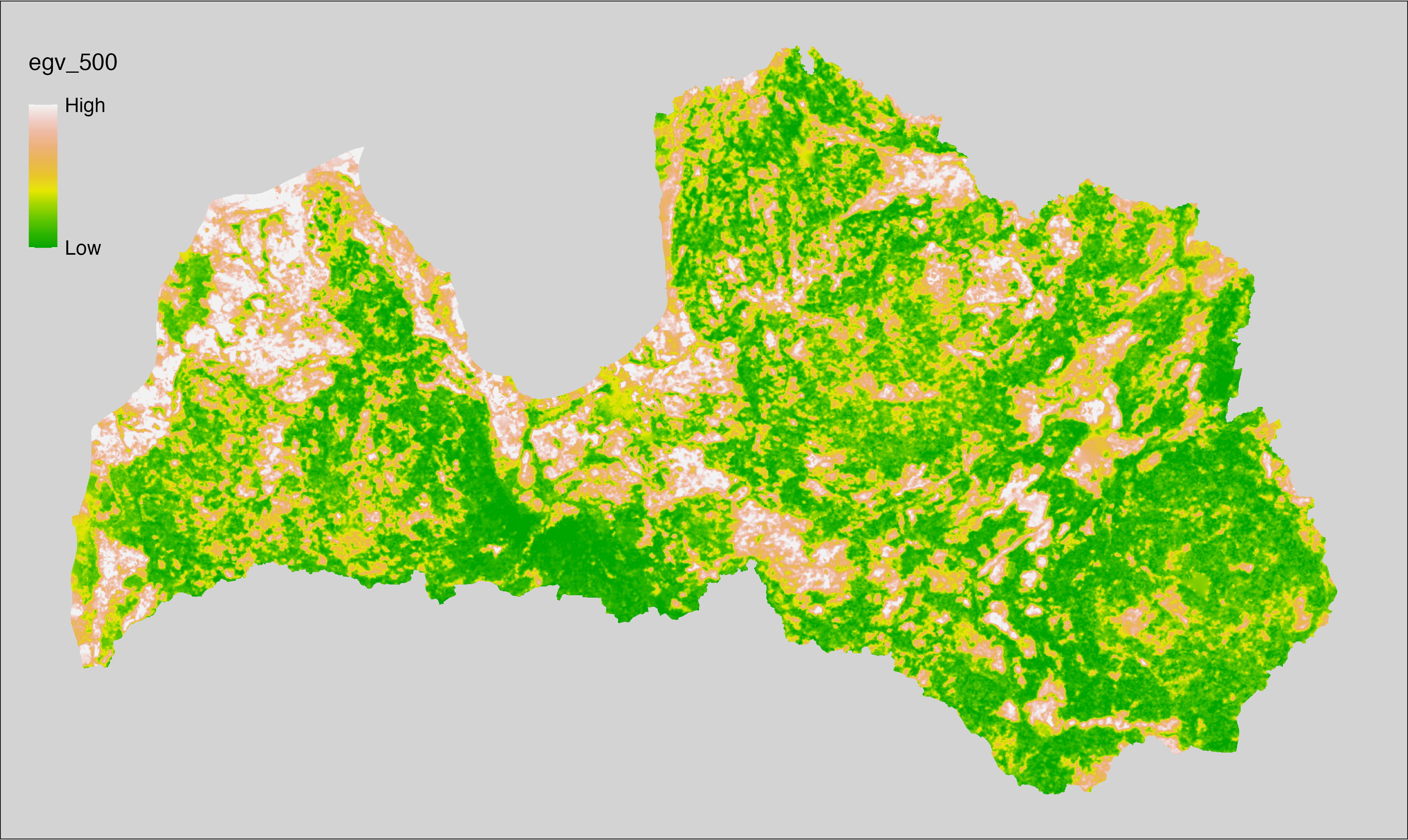
6.501 SoilChemistry_ESDAC-CaCo3_cell
filename: SoilChemistry_ESDAC-CaCo3_cell.tif
layername: egv_501
English name: Average value of Topsoil Calcium Carbonate Content (ESDAC v2.0) within the analysis cell (1 ha)
Latvian name: Augsnes virskārtas kalcija karbonātu saturs (ESDAC v2.0) analīzes šūnā (1 ha)
Procedure: Directly derived from the Soil chemistry. Processed
using the workflow egvtools::downscale2egv() with fill gaps = TRUE, performing
inverse distance weighted (power = 2) filling of gaps at the border
and smooth = FALSE. This is done to preserve the original values as much as
possible (bilinear interpolation is involved when projecting from a 500 m
resolution to a 100 m resolution in a different CRS). Finally, the layer is
standardised by subtracting the arithmetic mean and dividing by the root mean
squared error.
Code
# libs ----
if(!require(egvtools)) {remotes::install_github("aavotins/egvtools"); require(egvtools)}
# CaCO3 ----
egv=downscale2egv(
template_path = "./Templates/TemplateRasters/LV100m_10km.tif",
grid_path = "./Templates/TemplateGrids/tikls1km_sauzeme.parquet",
rawfile_path = "./Geodata/2024/Soils/ESDAC/chemistry/chemistry/Caco3/CaCO3.tif",
out_path = "./RasterGrids_100m/2024/RAW/",
file_name = "SoilChemistry_ESDAC-CaCo3_cell.tif",
layer_name = "egv_501",
fill_gaps = TRUE,
smooth = FALSE,
plot_result = TRUE)
egv
# standardisation ----
if(!require(terra)) {install.packages("terra"); require(terra)}
if(!require(tidyverse)) {install.packages("tidyverse"); require(tidyverse)}
nosaukums="SoilChemistry_ESDAC-CaCo3_cell.tif"
ielasisanas_cels=paste0("./RasterGrids_100m/2024/RAW/",nosaukums)
saglabasanas_cels=paste0("./RasterGrids_100m/2024/Scaled/",nosaukums)
slanis=rast(ielasisanas_cels)
videjais=global(slanis,fun="mean",na.rm=TRUE)
centrets=slanis-videjais[,1]
standartnovirze=terra::global(centrets,fun="rms",na.rm=TRUE)
merogots=centrets/standartnovirze[,1]
writeRaster(merogots,
filename=saglabasanas_cels,
overwrite=TRUE)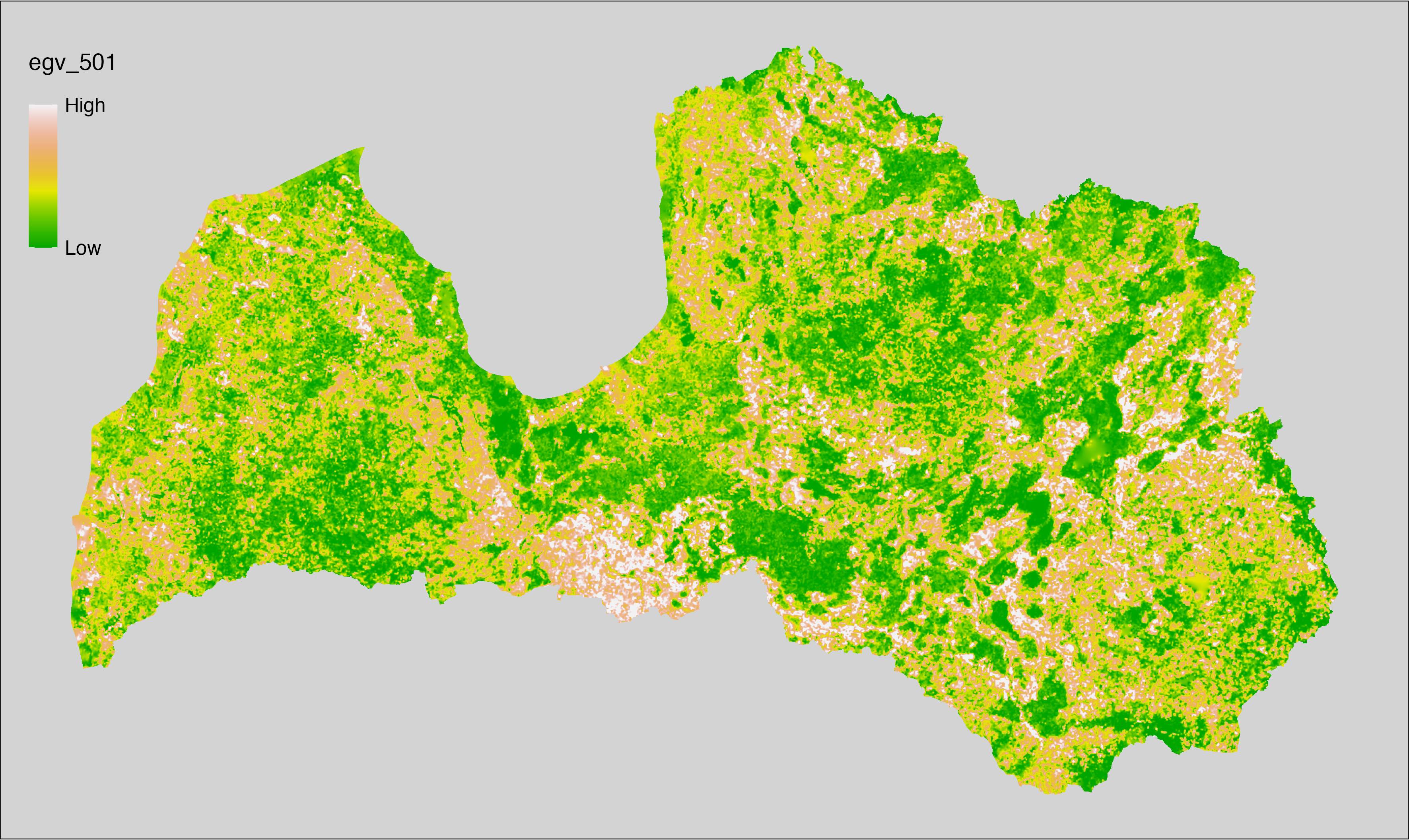
6.502 SoilChemistry_ESDAC-K_cell
filename: SoilChemistry_ESDAC-K_cell.tif
layername: egv_502
English name: Average value of Topsoil Potassium Content (ESDAC v2.0) within the analysis cell (1 ha)
Latvian name: Augsnes virskārtas kālija saturs (ESDAC v2.0) analīzes šūnā (1 ha)
Procedure: Directly derived from the Soil chemistry. Processed
using the workflow egvtools::downscale2egv() with fill gaps = TRUE, performing
inverse distance weighted (power = 2) filling of gaps at the border
and smooth = FALSE. This is done to preserve the original values as much as
possible (bilinear interpolation is involved when projecting from a 500 m
resolution to a 100 m resolution in a different CRS). Finally, the layer is
standardised by subtracting the arithmetic mean and dividing by the root mean
squared error.
Code
# libs ----
if(!require(egvtools)) {remotes::install_github("aavotins/egvtools"); require(egvtools)}
# K ----
egv=downscale2egv(
template_path = "./Templates/TemplateRasters/LV100m_10km.tif",
grid_path = "./Templates/TemplateGrids/tikls1km_sauzeme.parquet",
rawfile_path = "./Geodata/2024/Soils/ESDAC/chemistry/chemistry/K/K.tif",
out_path = "./RasterGrids_100m/2024/RAW/",
file_name = "SoilChemistry_ESDAC-K_cell.tif",
layer_name = "egv_502",
fill_gaps = TRUE,
smooth = FALSE,
plot_result = TRUE)
egv
# standardisation ----
if(!require(terra)) {install.packages("terra"); require(terra)}
if(!require(tidyverse)) {install.packages("tidyverse"); require(tidyverse)}
nosaukums="SoilChemistry_ESDAC-K_cell.tif"
ielasisanas_cels=paste0("./RasterGrids_100m/2024/RAW/",nosaukums)
saglabasanas_cels=paste0("./RasterGrids_100m/2024/Scaled/",nosaukums)
slanis=rast(ielasisanas_cels)
videjais=global(slanis,fun="mean",na.rm=TRUE)
centrets=slanis-videjais[,1]
standartnovirze=terra::global(centrets,fun="rms",na.rm=TRUE)
merogots=centrets/standartnovirze[,1]
writeRaster(merogots,
filename=saglabasanas_cels,
overwrite=TRUE)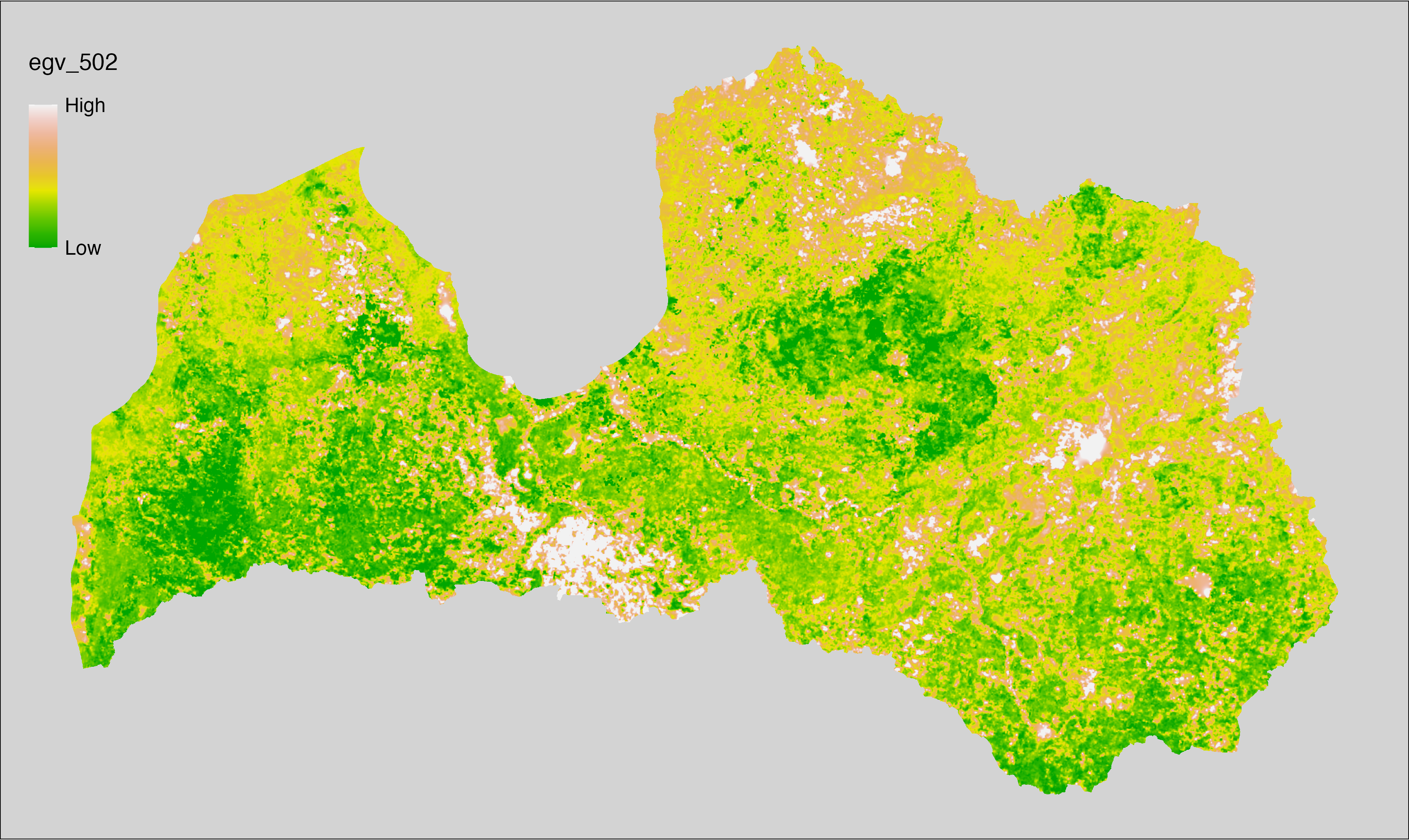
6.503 SoilChemistry_ESDAC-N_cell
filename: SoilChemistry_ESDAC-N_cell.tif
layername: egv_503
English name: Average value of Topsoil Nitrogen Content (ESDAC v2.0) within the analysis cell (1 ha)
Latvian name: Augsnes virskārtas slāpekļa saturs (ESDAC v2.0) analīzes šūnā (1 ha)
Procedure: Directly derived from the Soil chemistry. Processed
using the workflow egvtools::downscale2egv() with fill gaps = TRUE, performing
inverse distance weighted (power = 2) filling of gaps at the border
and smooth = FALSE. This is done to preserve the original values as much as
possible (bilinear interpolation is involved when projecting from a 500 m
resolution to a 100 m resolution in a different CRS). Finally, the layer is
standardised by subtracting the arithmetic mean and dividing by the root mean
squared error.
Code
# libs ----
if(!require(egvtools)) {remotes::install_github("aavotins/egvtools"); require(egvtools)}
# N ----
egv=downscale2egv(
template_path = "./Templates/TemplateRasters/LV100m_10km.tif",
grid_path = "./Templates/TemplateGrids/tikls1km_sauzeme.parquet",
rawfile_path = "./Geodata/2024/Soils/ESDAC/chemistry/chemistry/N/N.tif",
out_path = "./RasterGrids_100m/2024/RAW/",
file_name = "SoilChemistry_ESDAC-N_cell.tif",
layer_name = "egv_503",
fill_gaps = TRUE,
smooth = FALSE,
plot_result = TRUE)
egv
# standardisation ----
if(!require(terra)) {install.packages("terra"); require(terra)}
if(!require(tidyverse)) {install.packages("tidyverse"); require(tidyverse)}
nosaukums="SoilChemistry_ESDAC-N_cell.tif"
ielasisanas_cels=paste0("./RasterGrids_100m/2024/RAW/",nosaukums)
saglabasanas_cels=paste0("./RasterGrids_100m/2024/Scaled/",nosaukums)
slanis=rast(ielasisanas_cels)
videjais=global(slanis,fun="mean",na.rm=TRUE)
centrets=slanis-videjais[,1]
standartnovirze=terra::global(centrets,fun="rms",na.rm=TRUE)
merogots=centrets/standartnovirze[,1]
writeRaster(merogots,
filename=saglabasanas_cels,
overwrite=TRUE)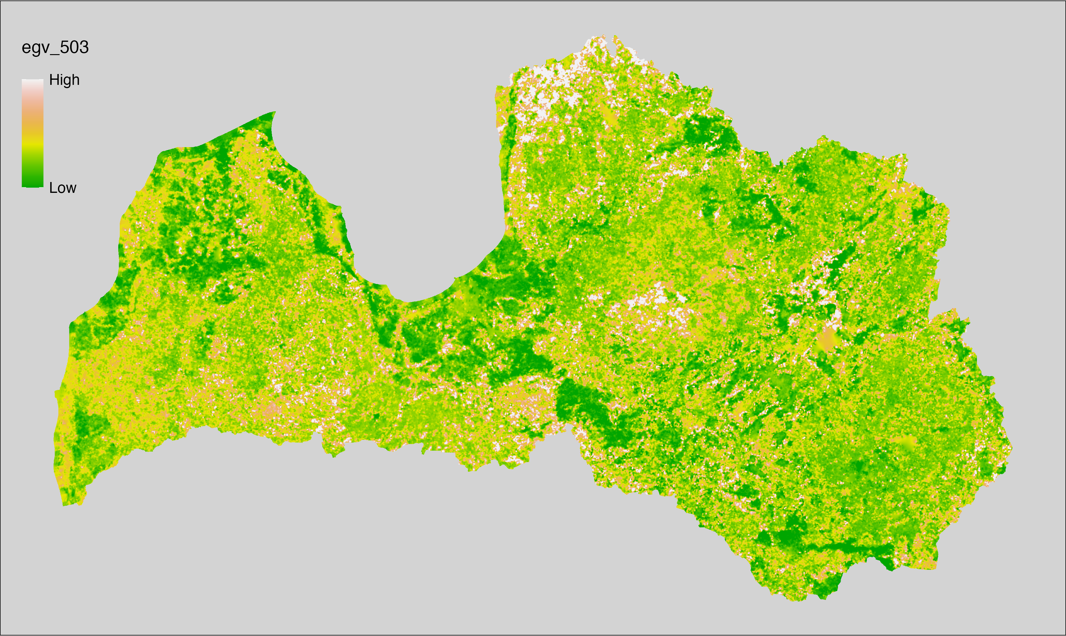
6.504 SoilChemistry_ESDAC-P_cell
filename: SoilChemistry_ESDAC-P_cell.tif
layername: egv_504
English name: Average value of Topsoil Phosphorous Content (ESDAC v2.0) within the analysis cell (1 ha)
Latvian name: Augsnes virskārtas fosfora saturs (ESDAC v2.0) analīzes šūnā (1 ha)
Procedure: Directly derived from the Soil chemistry. Processed
using the workflow egvtools::downscale2egv() with fill gaps = TRUE, performing
inverse distance weighted (power = 2) filling of gaps at the border
and smooth = FALSE. This is done to preserve the original values as much as
possible (bilinear interpolation is involved when projecting from a 500 m
resolution to a 100 m resolution in a different CRS). Finally, the layer is
standardised by subtracting the arithmetic mean and dividing by the root mean
squared error.
Code
# libs ----
if(!require(egvtools)) {remotes::install_github("aavotins/egvtools"); require(egvtools)}
# P ----
egv=downscale2egv(
template_path = "./Templates/TemplateRasters/LV100m_10km.tif",
grid_path = "./Templates/TemplateGrids/tikls1km_sauzeme.parquet",
rawfile_path = "./Geodata/2024/Soils/ESDAC/chemistry/chemistry/P/P.tif",
out_path = "./RasterGrids_100m/2024/RAW/",
file_name = "SoilChemistry_ESDAC-P_cell.tif",
layer_name = "egv_504",
fill_gaps = TRUE,
smooth = FALSE,
plot_result = TRUE)
egv
# standardisation ----
if(!require(terra)) {install.packages("terra"); require(terra)}
if(!require(tidyverse)) {install.packages("tidyverse"); require(tidyverse)}
nosaukums="SoilChemistry_ESDAC-P_cell.tif"
ielasisanas_cels=paste0("./RasterGrids_100m/2024/RAW/",nosaukums)
saglabasanas_cels=paste0("./RasterGrids_100m/2024/Scaled/",nosaukums)
slanis=rast(ielasisanas_cels)
videjais=global(slanis,fun="mean",na.rm=TRUE)
centrets=slanis-videjais[,1]
standartnovirze=terra::global(centrets,fun="rms",na.rm=TRUE)
merogots=centrets/standartnovirze[,1]
writeRaster(merogots,
filename=saglabasanas_cels,
overwrite=TRUE)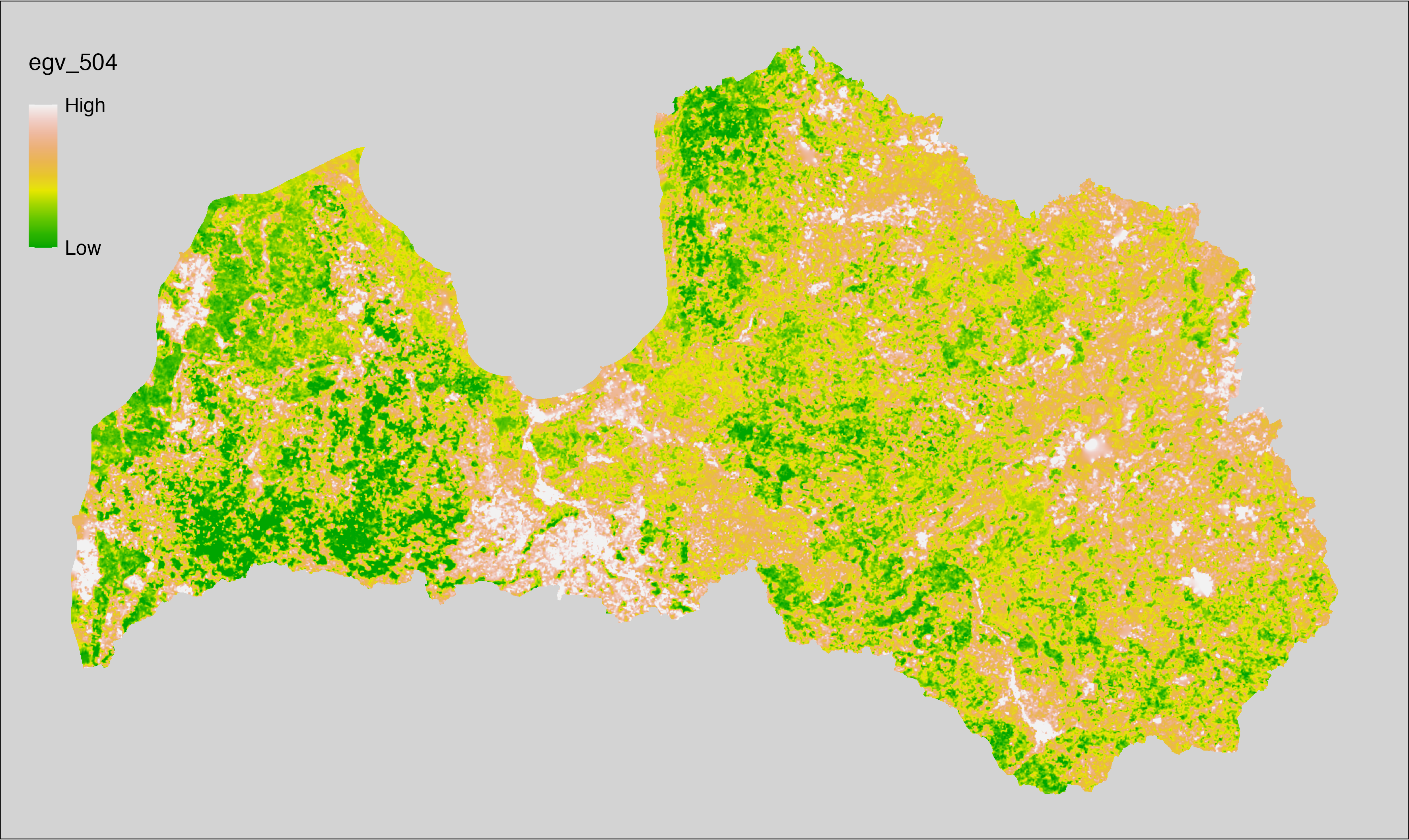
6.505 SoilChemistry_ESDAC-phH2O_cell
filename: SoilChemistry_ESDAC-phH2O_cell.tif
layername: egv_505
English name: Average value of Topsoil pH reaction in water (ESDAC v2.0) within the analysis cell (1 ha)
Latvian name: Augsnes virskārtas reakcija (pH) ūdens šķīdumā (ESDAC v2.0) analīzes šūnā (1 ha)
Procedure: Directly derived from the Soil chemistry. Processed
using the workflow egvtools::downscale2egv() with fill gaps = TRUE, performing
inverse distance weighted (power = 2) filling of gaps at the border
and smooth = FALSE. This is done to preserve the original values as much as
possible (bilinear interpolation is involved when projecting from a 500 m
resolution to a 100 m resolution in a different CRS). Finally, the layer is
standardised by subtracting the arithmetic mean and dividing by the root mean
squared error.
Code
# libs ----
if(!require(egvtools)) {remotes::install_github("aavotins/egvtools"); require(egvtools)}
# pH_H2O ----
egv=downscale2egv(
template_path = "./Templates/TemplateRasters/LV100m_10km.tif",
grid_path = "./Templates/TemplateGrids/tikls1km_sauzeme.parquet",
rawfile_path = "./Geodata/2024/Soils/ESDAC/chemistry/chemistry/pH_H2O/pH_H2O.tif",
out_path = "./RasterGrids_100m/2024/RAW/",
file_name = "SoilChemistry_ESDAC-phH2O_cell.tif",
layer_name = "egv_505",
fill_gaps = TRUE,
smooth = FALSE,
plot_result = TRUE)
egv
# standardisation ----
if(!require(terra)) {install.packages("terra"); require(terra)}
if(!require(tidyverse)) {install.packages("tidyverse"); require(tidyverse)}
nosaukums="SoilChemistry_ESDAC-phH2O_cell.tif"
ielasisanas_cels=paste0("./RasterGrids_100m/2024/RAW/",nosaukums)
saglabasanas_cels=paste0("./RasterGrids_100m/2024/Scaled/",nosaukums)
slanis=rast(ielasisanas_cels)
videjais=global(slanis,fun="mean",na.rm=TRUE)
centrets=slanis-videjais[,1]
standartnovirze=terra::global(centrets,fun="rms",na.rm=TRUE)
merogots=centrets/standartnovirze[,1]
writeRaster(merogots,
filename=saglabasanas_cels,
overwrite=TRUE)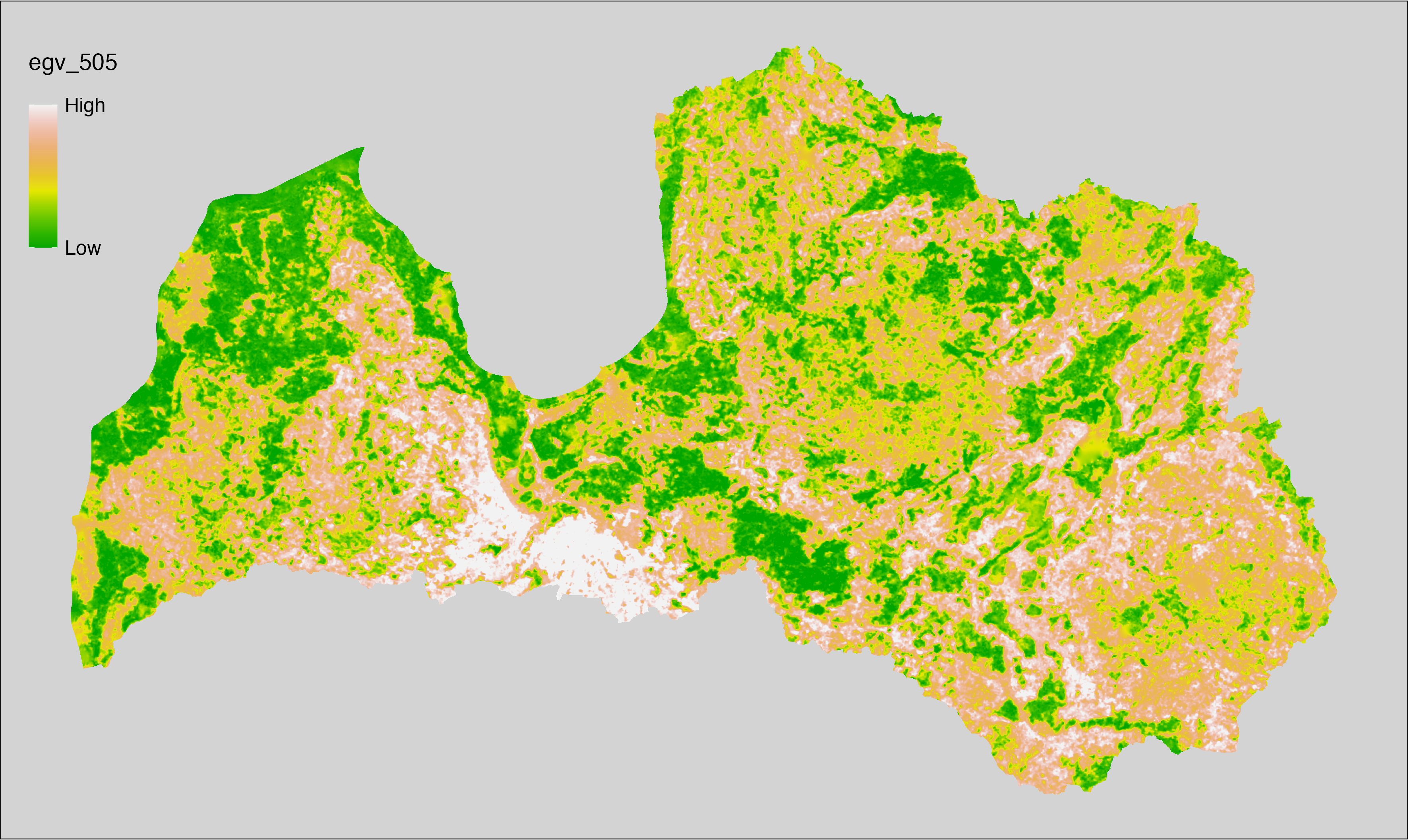
6.506 SoilTexture_Clay_cell
filename: SoilTexture_Clay_cell.tif
layername: egv_506
English name: Fractional cover of Clay Soils within the analysis cell (1 ha)
Latvian name: Augsnes granulometriskās klases “māls” platības īpatsvars analīzes šūnā (1 ha)
Procedure: Derived from the Soil texture product. First, the layer is
reclassified so that the class of interest is 1 and the other classes are 0. The resulting layer
is then aggregated to EGV resolution using the workflow egvtools::input2egv(), which
calculates the arithmetic mean to determine the cover fraction. During
aggregation, inverse distance weighted (power = 2) gap filling on the output is
applied to ensure no missing values at the edges. Finally, the layer is
standardised by subtracting the arithmetic mean and dividing by the root mean squared
error.
Code
# libs ----
if(!require(terra)) {install.packages("terra"); require(terra)}
if(!require(egvtools)) {remotes::install_github("aavotins/egvtools"); require(egvtools)}
# templates ----
template10=rast("./Templates/TemplateRasters/LV10m_10km.tif")
template100=rast("./Templates/TemplateRasters/LV100m_10km.tif")
# input ----
combtext=rast("./RasterGrids_10m/2024/SoilTXT_combined.tif")
# EGVs cell ----
# SoilTexture_Clay_cell.tif egv_506
clay10=ifel(combtext==3,1,0)
input2egv(input=clay10,
egv_template="./Templates/TemplateRasters/LV100m_10km.tif",
summary_function = "average",
missing_job = "FillOutput",
idw_weight = 2,
outlocation = "./RasterGrids_100m/2024/RAW/",
outfilename = "SoilTexture_Clay_cell.tif",
layername="egv_506",
return_visible = TRUE)
# standardisation ----
if(!require(terra)) {install.packages("terra"); require(terra)}
if(!require(tidyverse)) {install.packages("tidyverse"); require(tidyverse)}
nosaukums="SoilTexture_Clay_cell.tif"
ielasisanas_cels=paste0("./RasterGrids_100m/2024/RAW/",nosaukums)
saglabasanas_cels=paste0("./RasterGrids_100m/2024/Scaled/",nosaukums)
slanis=rast(ielasisanas_cels)
videjais=global(slanis,fun="mean",na.rm=TRUE)
centrets=slanis-videjais[,1]
standartnovirze=terra::global(centrets,fun="rms",na.rm=TRUE)
merogots=centrets/standartnovirze[,1]
writeRaster(merogots,
filename=saglabasanas_cels,
overwrite=TRUE)
6.507 SoilTexture_Clay_r500
filename: SoilTexture_Clay_r500.tif
layername: egv_507
English name: Fractional cover of Clay Soils within the 0.5 km landscape
Latvian name: Augsnes granulometriskās klases “māls” platības īpatsvars 0,5 km ainavā
Procedure: The cover fraction within a radius of 500 m around the analysis grid cell is
calculated as the area-weighted sum of the analysis cells inside the
buffer, using the workflow egvtools::radius_function(). During the calculation of the landscape metric,
inverse distance weighted (power = 2) gap filling on the output is applied
to ensure no missing values at the edges. Then the layer is rewritten to set
its name. Finally, the layer is standardised by subtracting the arithmetic
mean and dividing by the root mean squared error.
Code
# libs ----
if(!require(terra)) {install.packages("terra"); require(terra)}
if(!require(egvtools)) {remotes::install_github("aavotins/egvtools"); require(egvtools)}
# EGVs radii ----
radius_function(
kvadrati_path = "./Templates/TemplateGrids/tiles/",
radii_path = "./Templates/TemplateGridPoints/tiles/",
tikls100_path = "./Templates/TemplateGrids/tikls100_sauzeme.parquet",
template_path = "./Templates/TemplateRasters/LV100m_10km.tif",
input_layers = c("./RasterGrids_100m/2024/RAW/SoilTexture_Clay_cell.tif"),
layer_prefixes = c("SoilTexture_Clay"),
output_dir = "./RasterGrids_100m/2024/RAW/",
n_workers = 5,
radii = c("r500"),
radius_mode = "sparse",
extract_fun = "mean",
fill_missing = TRUE,
IDW_weight = 2,
future_max_size = 5 * 1024^3)
# SoilTexture_Clay_r500.tif egv_507
slanis=rast("./RasterGrids_100m/2024/RAW/SoilTexture_Clay_r500.tif")
names(slanis)="egv_507"
slanis2=project(slanis,template100)
writeRaster(slanis2,
"./RasterGrids_100m/2024/RAW/SoilTexture_Clay_r500.tif",
overwrite=TRUE)
# standardisation ----
if(!require(terra)) {install.packages("terra"); require(terra)}
if(!require(tidyverse)) {install.packages("tidyverse"); require(tidyverse)}
nosaukums="SoilTexture_Clay_r500.tif"
ielasisanas_cels=paste0("./RasterGrids_100m/2024/RAW/",nosaukums)
saglabasanas_cels=paste0("./RasterGrids_100m/2024/Scaled/",nosaukums)
slanis=rast(ielasisanas_cels)
videjais=global(slanis,fun="mean",na.rm=TRUE)
centrets=slanis-videjais[,1]
standartnovirze=terra::global(centrets,fun="rms",na.rm=TRUE)
merogots=centrets/standartnovirze[,1]
writeRaster(merogots,
filename=saglabasanas_cels,
overwrite=TRUE)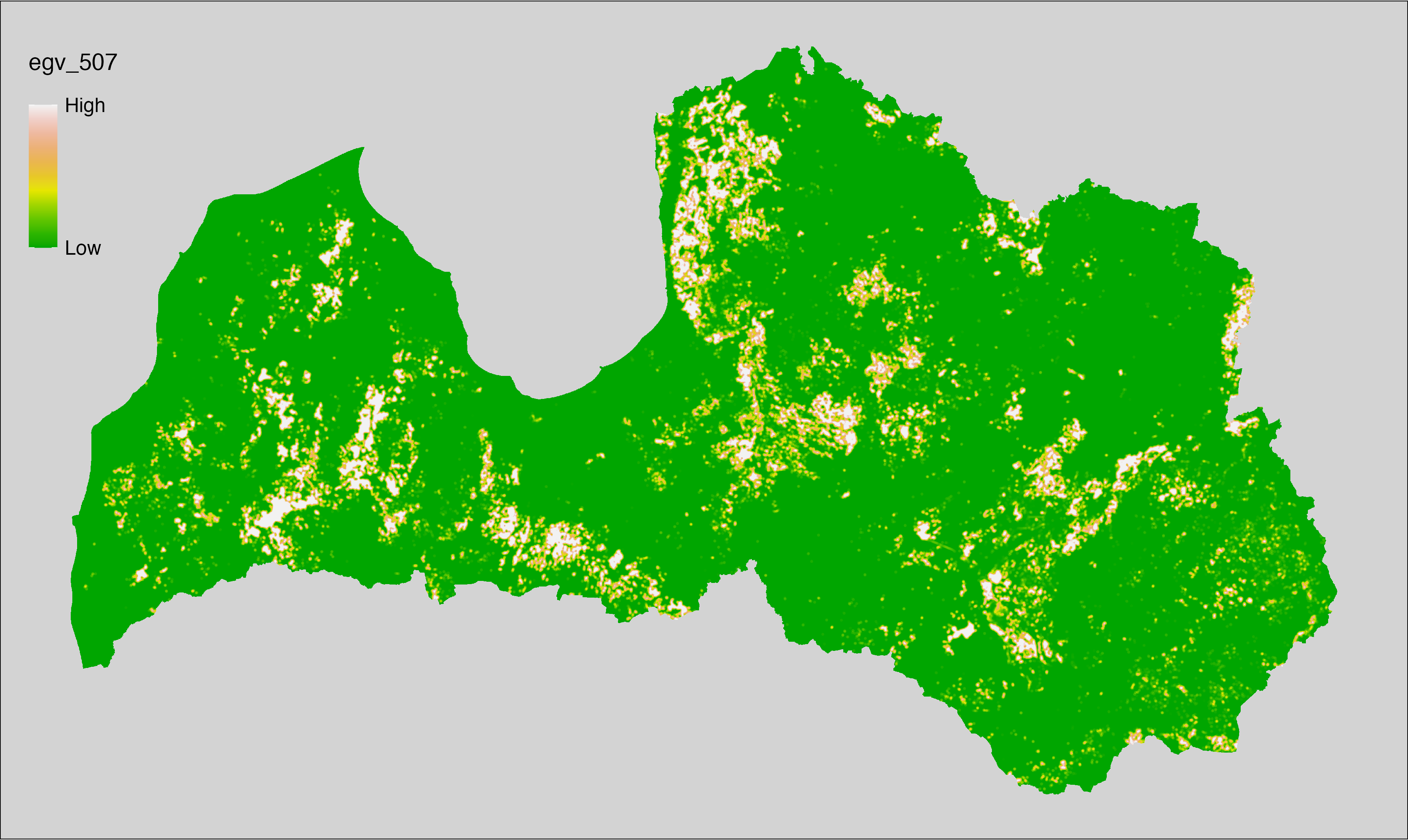
6.508 SoilTexture_Clay_r1250
filename: SoilTexture_Clay_r1250.tif
layername: egv_508
English name: Fractional cover of Clay Soils within the 1.25 km landscape
Latvian name: Augsnes granulometriskās klases “māls” platības īpatsvars 1,25 km ainavā
Procedure: The cover fraction within a radius of 1250 m around the analysis grid cell is
calculated as the area-weighted sum of the analysis cells inside the
buffer, using the workflow egvtools::radius_function(). During the calculation of the landscape metric,
inverse distance weighted (power = 2) gap filling on the output is applied
to ensure no missing values at the edges. Then the layer is rewritten to set
its name. Finally, the layer is standardised by subtracting the arithmetic
mean and dividing by the root mean squared error.
Code
# libs ----
if(!require(terra)) {install.packages("terra"); require(terra)}
if(!require(egvtools)) {remotes::install_github("aavotins/egvtools"); require(egvtools)}
# EGVs radii ----
radius_function(
kvadrati_path = "./Templates/TemplateGrids/tiles/",
radii_path = "./Templates/TemplateGridPoints/tiles/",
tikls100_path = "./Templates/TemplateGrids/tikls100_sauzeme.parquet",
template_path = "./Templates/TemplateRasters/LV100m_10km.tif",
input_layers = c("./RasterGrids_100m/2024/RAW/SoilTexture_Clay_cell.tif"),
layer_prefixes = c("SoilTexture_Clay"),
output_dir = "./RasterGrids_100m/2024/RAW/",
n_workers = 5,
radii = c("r1250"),
radius_mode = "sparse",
extract_fun = "mean",
fill_missing = TRUE,
IDW_weight = 2,
future_max_size = 5 * 1024^3)
# SoilTexture_Clay_r1250.tif egv_508
slanis=rast("./RasterGrids_100m/2024/RAW/SoilTexture_Clay_r1250.tif")
names(slanis)="egv_508"
slanis2=project(slanis,template100)
writeRaster(slanis2,
"./RasterGrids_100m/2024/RAW/SoilTexture_Clay_r1250.tif",
overwrite=TRUE)
# standardisation ----
if(!require(terra)) {install.packages("terra"); require(terra)}
if(!require(tidyverse)) {install.packages("tidyverse"); require(tidyverse)}
nosaukums="SoilTexture_Clay_r1250.tif"
ielasisanas_cels=paste0("./RasterGrids_100m/2024/RAW/",nosaukums)
saglabasanas_cels=paste0("./RasterGrids_100m/2024/Scaled/",nosaukums)
slanis=rast(ielasisanas_cels)
videjais=global(slanis,fun="mean",na.rm=TRUE)
centrets=slanis-videjais[,1]
standartnovirze=terra::global(centrets,fun="rms",na.rm=TRUE)
merogots=centrets/standartnovirze[,1]
writeRaster(merogots,
filename=saglabasanas_cels,
overwrite=TRUE)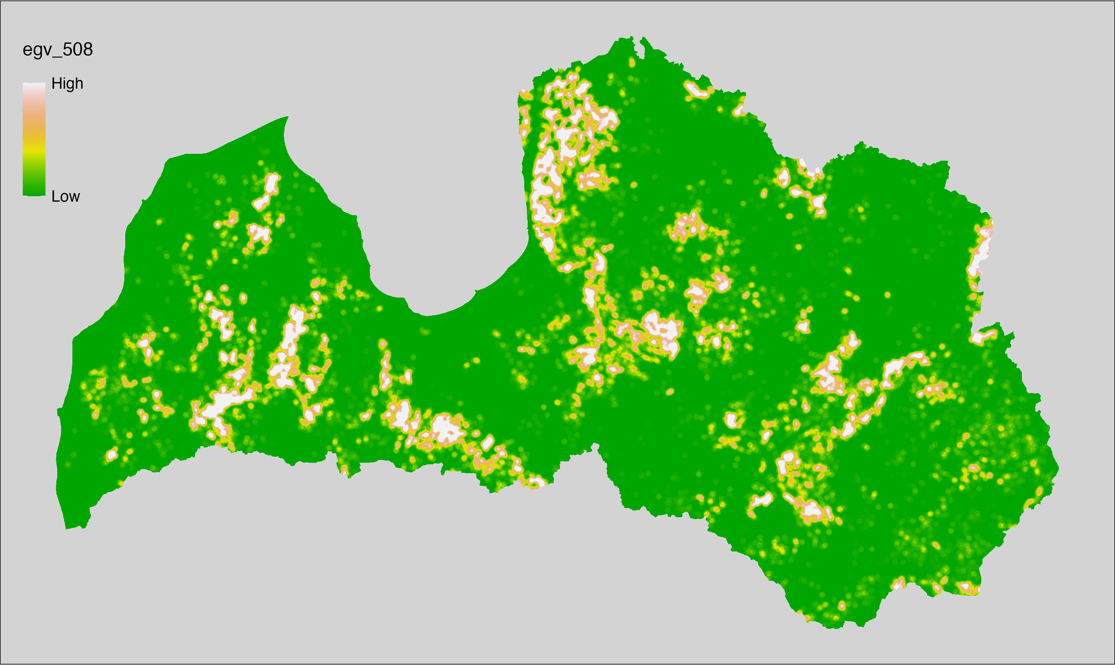
6.509 SoilTexture_Clay_r3000
filename: SoilTexture_Clay_r3000.tif
layername: egv_509
English name: Fractional cover of Clay Soils within the 3 km landscape
Latvian name: Augsnes granulometriskās klases “māls” platības īpatsvars 3 km ainavā
Procedure: The cover fraction within a radius of 3000 m around the analysis grid cell is
calculated as the area-weighted sum of the analysis cells inside the
buffer, using the workflow egvtools::radius_function(). During the calculation of the landscape metric,
inverse distance weighted (power = 2) gap filling on the output is applied
to ensure no missing values at the edges. Then the layer is rewritten to set
its name. Finally, the layer is standardised by subtracting the arithmetic
mean and dividing by the root mean squared error.
Code
# libs ----
if(!require(terra)) {install.packages("terra"); require(terra)}
if(!require(egvtools)) {remotes::install_github("aavotins/egvtools"); require(egvtools)}
# EGVs radii ----
radius_function(
kvadrati_path = "./Templates/TemplateGrids/tiles/",
radii_path = "./Templates/TemplateGridPoints/tiles/",
tikls100_path = "./Templates/TemplateGrids/tikls100_sauzeme.parquet",
template_path = "./Templates/TemplateRasters/LV100m_10km.tif",
input_layers = c("./RasterGrids_100m/2024/RAW/SoilTexture_Clay_cell.tif"),
layer_prefixes = c("SoilTexture_Clay"),
output_dir = "./RasterGrids_100m/2024/RAW/",
n_workers = 5,
radii = c("r3000"),
radius_mode = "sparse",
extract_fun = "mean",
fill_missing = TRUE,
IDW_weight = 2,
future_max_size = 5 * 1024^3)
# SoilTexture_Clay_r3000.tif egv_509
slanis=rast("./RasterGrids_100m/2024/RAW/SoilTexture_Clay_r3000.tif")
names(slanis)="egv_509"
slanis2=project(slanis,template100)
writeRaster(slanis2,
"./RasterGrids_100m/2024/RAW/SoilTexture_Clay_r3000.tif",
overwrite=TRUE)
# standardisation ----
if(!require(terra)) {install.packages("terra"); require(terra)}
if(!require(tidyverse)) {install.packages("tidyverse"); require(tidyverse)}
nosaukums="SoilTexture_Clay_r3000.tif"
ielasisanas_cels=paste0("./RasterGrids_100m/2024/RAW/",nosaukums)
saglabasanas_cels=paste0("./RasterGrids_100m/2024/Scaled/",nosaukums)
slanis=rast(ielasisanas_cels)
videjais=global(slanis,fun="mean",na.rm=TRUE)
centrets=slanis-videjais[,1]
standartnovirze=terra::global(centrets,fun="rms",na.rm=TRUE)
merogots=centrets/standartnovirze[,1]
writeRaster(merogots,
filename=saglabasanas_cels,
overwrite=TRUE)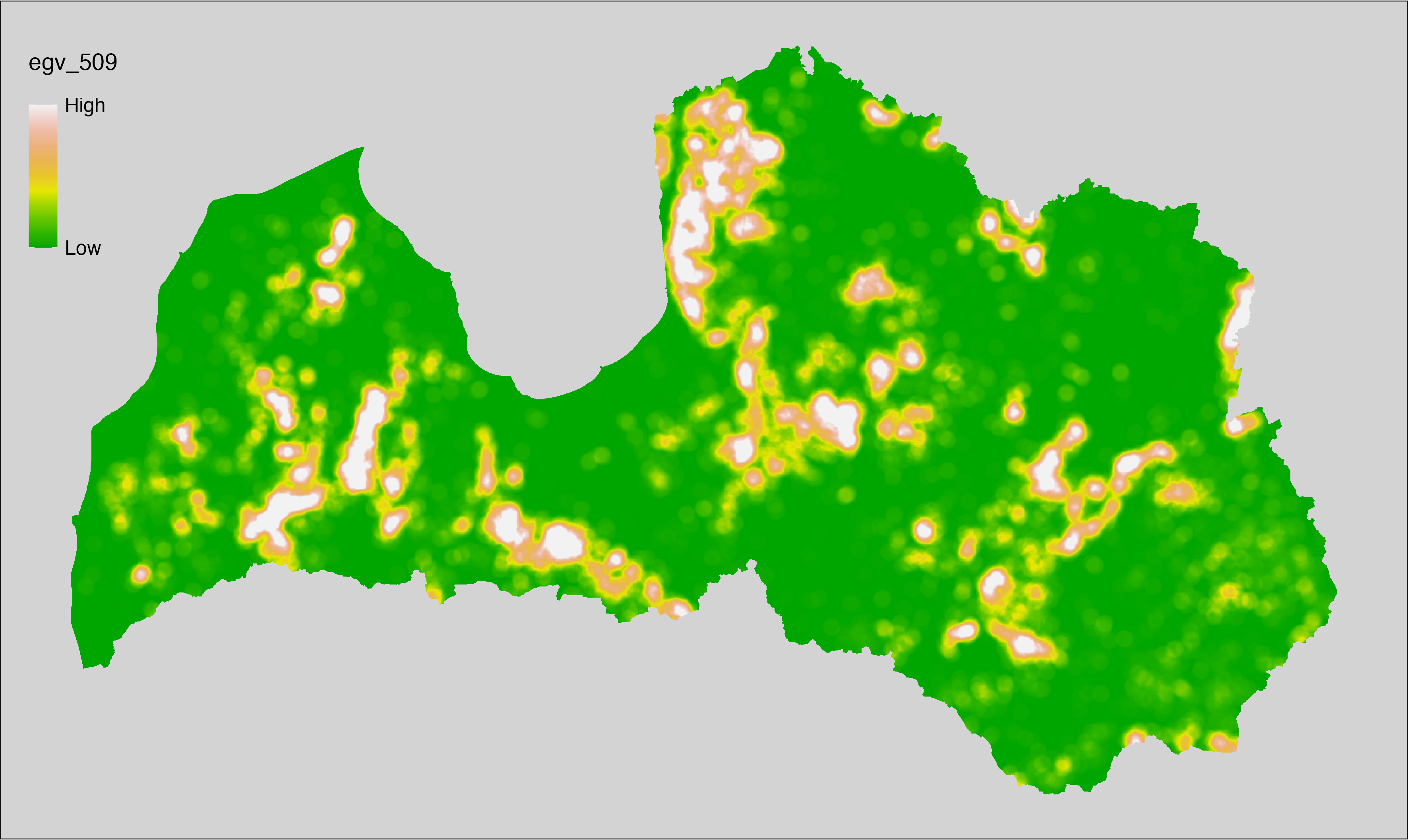
6.510 SoilTexture_Clay_r10000
filename: SoilTexture_Clay_r10000.tif
layername: egv_510
English name: Fractional cover of Clay Soils within the 10 km landscape
Latvian name: Augsnes granulometriskās klases “māls” platības īpatsvars 10 km ainavā
Procedure: The cover fraction within a radius of 10000 m around the analysis grid cell is
calculated as the area-weighted sum of the analysis cells inside the
buffer, using the workflow egvtools::radius_function(). During the calculation of the landscape metric,
inverse distance weighted (power = 2) gap filling on the output is applied
to ensure no missing values at the edges. Then the layer is rewritten to set
its name. Finally, the layer is standardised by subtracting the arithmetic
mean and dividing by the root mean squared error.
Code
# libs ----
if(!require(terra)) {install.packages("terra"); require(terra)}
if(!require(egvtools)) {remotes::install_github("aavotins/egvtools"); require(egvtools)}
# EGVs radii ----
radius_function(
kvadrati_path = "./Templates/TemplateGrids/tiles/",
radii_path = "./Templates/TemplateGridPoints/tiles/",
tikls100_path = "./Templates/TemplateGrids/tikls100_sauzeme.parquet",
template_path = "./Templates/TemplateRasters/LV100m_10km.tif",
input_layers = c("./RasterGrids_100m/2024/RAW/SoilTexture_Clay_cell.tif"),
layer_prefixes = c("SoilTexture_Clay"),
output_dir = "./RasterGrids_100m/2024/RAW/",
n_workers = 5,
radii = c("r10000"),
radius_mode = "sparse",
extract_fun = "mean",
fill_missing = TRUE,
IDW_weight = 2,
future_max_size = 5 * 1024^3)
# SoilTexture_Clay_r10000.tif egv_510
slanis=rast("./RasterGrids_100m/2024/RAW/SoilTexture_Clay_r10000.tif")
names(slanis)="egv_510"
slanis2=project(slanis,template100)
writeRaster(slanis2,
"./RasterGrids_100m/2024/RAW/SoilTexture_Clay_r10000.tif",
overwrite=TRUE)
# standardisation ----
if(!require(terra)) {install.packages("terra"); require(terra)}
if(!require(tidyverse)) {install.packages("tidyverse"); require(tidyverse)}
nosaukums="SoilTexture_Clay_r10000.tif"
ielasisanas_cels=paste0("./RasterGrids_100m/2024/RAW/",nosaukums)
saglabasanas_cels=paste0("./RasterGrids_100m/2024/Scaled/",nosaukums)
slanis=rast(ielasisanas_cels)
videjais=global(slanis,fun="mean",na.rm=TRUE)
centrets=slanis-videjais[,1]
standartnovirze=terra::global(centrets,fun="rms",na.rm=TRUE)
merogots=centrets/standartnovirze[,1]
writeRaster(merogots,
filename=saglabasanas_cels,
overwrite=TRUE)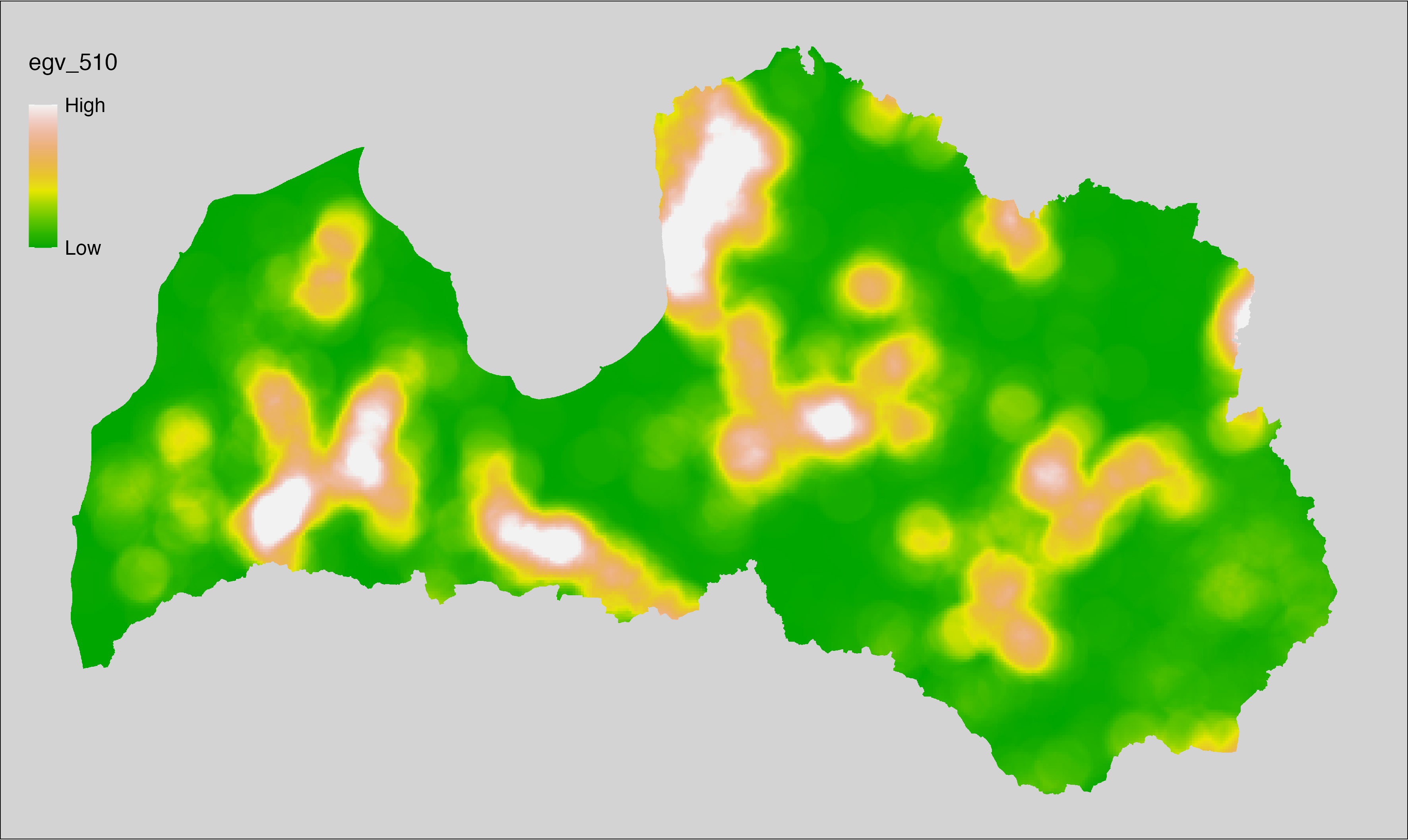
6.511 SoilTexture_Organic_cell
filename: SoilTexture_Organic_cell.tif
layername: egv_511
English name: Fractional cover of Organic Soils within the analysis cell (1 ha)
Latvian name: Augsnes granulometriskās klases “organiskās augsnes” platības īpatsvars analīzes šūnā (1 ha)
Procedure: Derived from the Soil texture product. First, the layer is
reclassified so that the class of interest is 1 and the other classes are 0. The resulting layer
is then aggregated to EGV resolution using the workflow egvtools::input2egv(), which
calculates the arithmetic mean to determine the cover fraction. During
aggregation, inverse distance weighted (power = 2) gap filling on the output is
applied to ensure no missing values at the edges. Finally, the layer is
standardised by subtracting the arithmetic mean and dividing by the root mean squared
error.
Code
# libs ----
if(!require(terra)) {install.packages("terra"); require(terra)}
if(!require(egvtools)) {remotes::install_github("aavotins/egvtools"); require(egvtools)}
# templates ----
template10=rast("./Templates/TemplateRasters/LV10m_10km.tif")
template100=rast("./Templates/TemplateRasters/LV100m_10km.tif")
# input ----
combtext=rast("./RasterGrids_10m/2024/SoilTXT_combined.tif")
# EGVs cell ----
# SoilTexture_Organic_cell.tif egv_511
org10=ifel(combtext==4,1,0)
input2egv(input=org10,
egv_template="./Templates/TemplateRasters/LV100m_10km.tif",
summary_function = "average",
missing_job = "FillOutput",
idw_weight = 2,
outlocation = "./RasterGrids_100m/2024/RAW/",
outfilename = "SoilTexture_Organic_cell.tif",
layername="egv_511",
return_visible = TRUE)
# standardisation ----
if(!require(terra)) {install.packages("terra"); require(terra)}
if(!require(tidyverse)) {install.packages("tidyverse"); require(tidyverse)}
nosaukums="SoilTexture_Organic_cell.tif"
ielasisanas_cels=paste0("./RasterGrids_100m/2024/RAW/",nosaukums)
saglabasanas_cels=paste0("./RasterGrids_100m/2024/Scaled/",nosaukums)
slanis=rast(ielasisanas_cels)
videjais=global(slanis,fun="mean",na.rm=TRUE)
centrets=slanis-videjais[,1]
standartnovirze=terra::global(centrets,fun="rms",na.rm=TRUE)
merogots=centrets/standartnovirze[,1]
writeRaster(merogots,
filename=saglabasanas_cels,
overwrite=TRUE)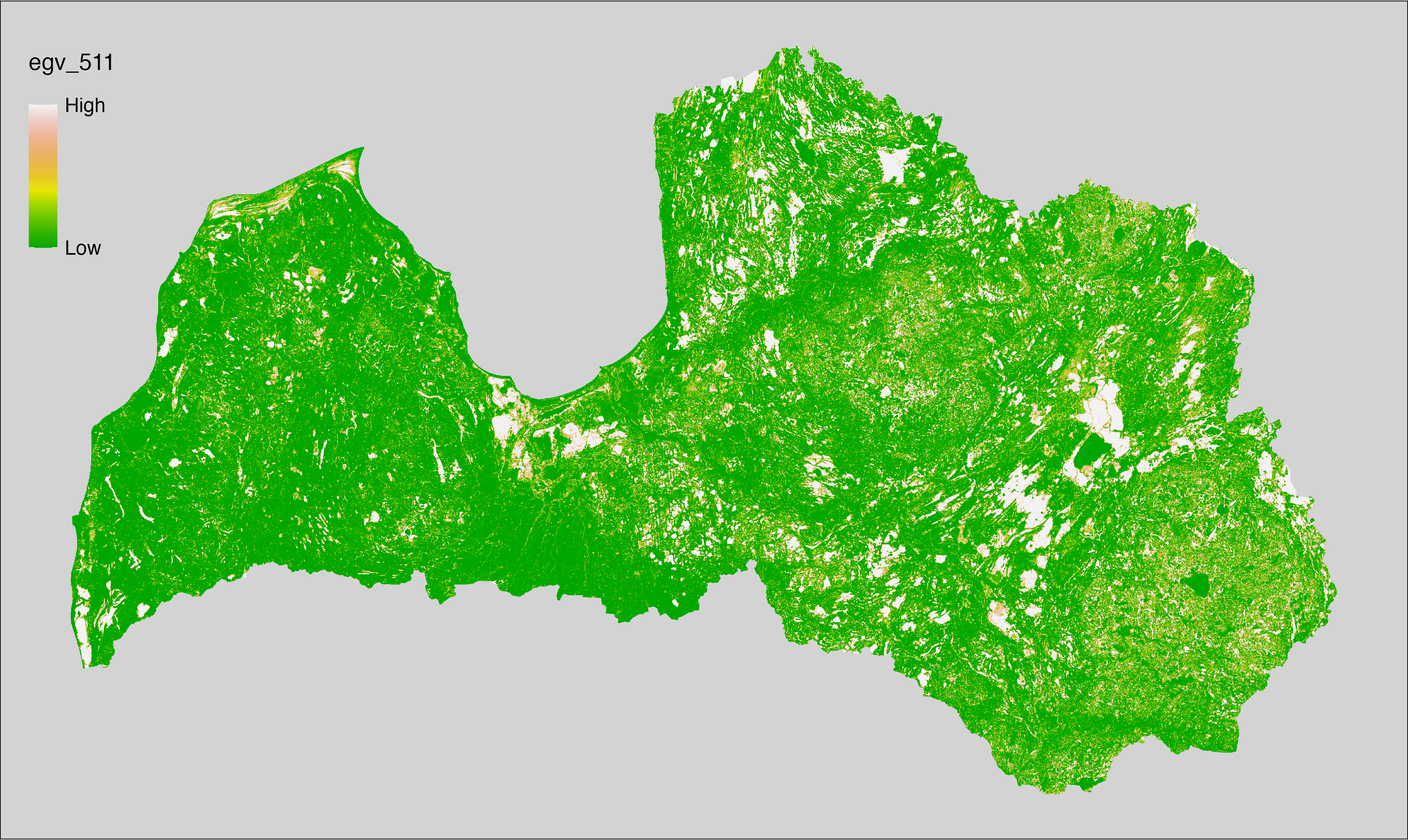
6.512 SoilTexture_Organic_r500
filename: SoilTexture_Organic_r500.tif
layername: egv_512
English name: Fractional cover of Organic Soils within the 0.5 km landscape
Latvian name: Augsnes granulometriskās klases “organiskās augsnes” platības īpatsvars 0,5 km ainavā
Procedure: The cover fraction within a radius of 500 m around the analysis grid cell is
calculated as the area-weighted sum of the analysis cells inside the
buffer, using the workflow egvtools::radius_function(). During the calculation of the landscape metric,
inverse distance weighted (power = 2) gap filling on the output is applied
to ensure no missing values at the edges. Then the layer is rewritten to set
its name. Finally, the layer is standardised by subtracting the arithmetic
mean and dividing by the root mean squared error.
Code
# libs ----
if(!require(terra)) {install.packages("terra"); require(terra)}
if(!require(egvtools)) {remotes::install_github("aavotins/egvtools"); require(egvtools)}
# EGVs radii ----
radius_function(
kvadrati_path = "./Templates/TemplateGrids/tiles/",
radii_path = "./Templates/TemplateGridPoints/tiles/",
tikls100_path = "./Templates/TemplateGrids/tikls100_sauzeme.parquet",
template_path = "./Templates/TemplateRasters/LV100m_10km.tif",
input_layers = c("./RasterGrids_100m/2024/RAW/SoilTexture_Organic_cell.tif"),
layer_prefixes = c("SoilTexture_Organic"),
output_dir = "./RasterGrids_100m/2024/RAW/",
n_workers = 5,
radii = c("r500"),
radius_mode = "sparse",
extract_fun = "mean",
fill_missing = TRUE,
IDW_weight = 2,
future_max_size = 5 * 1024^3)
# SoilTexture_Organic_r500.tif egv_512
slanis=rast("./RasterGrids_100m/2024/RAW/SoilTexture_Organic_r500.tif")
names(slanis)="egv_512"
slanis2=project(slanis,template100)
writeRaster(slanis2,
"./RasterGrids_100m/2024/RAW/SoilTexture_Organic_r500.tif",
overwrite=TRUE)
# standardisation ----
if(!require(terra)) {install.packages("terra"); require(terra)}
if(!require(tidyverse)) {install.packages("tidyverse"); require(tidyverse)}
nosaukums="SoilTexture_Organic_r500.tif"
ielasisanas_cels=paste0("./RasterGrids_100m/2024/RAW/",nosaukums)
saglabasanas_cels=paste0("./RasterGrids_100m/2024/Scaled/",nosaukums)
slanis=rast(ielasisanas_cels)
videjais=global(slanis,fun="mean",na.rm=TRUE)
centrets=slanis-videjais[,1]
standartnovirze=terra::global(centrets,fun="rms",na.rm=TRUE)
merogots=centrets/standartnovirze[,1]
writeRaster(merogots,
filename=saglabasanas_cels,
overwrite=TRUE)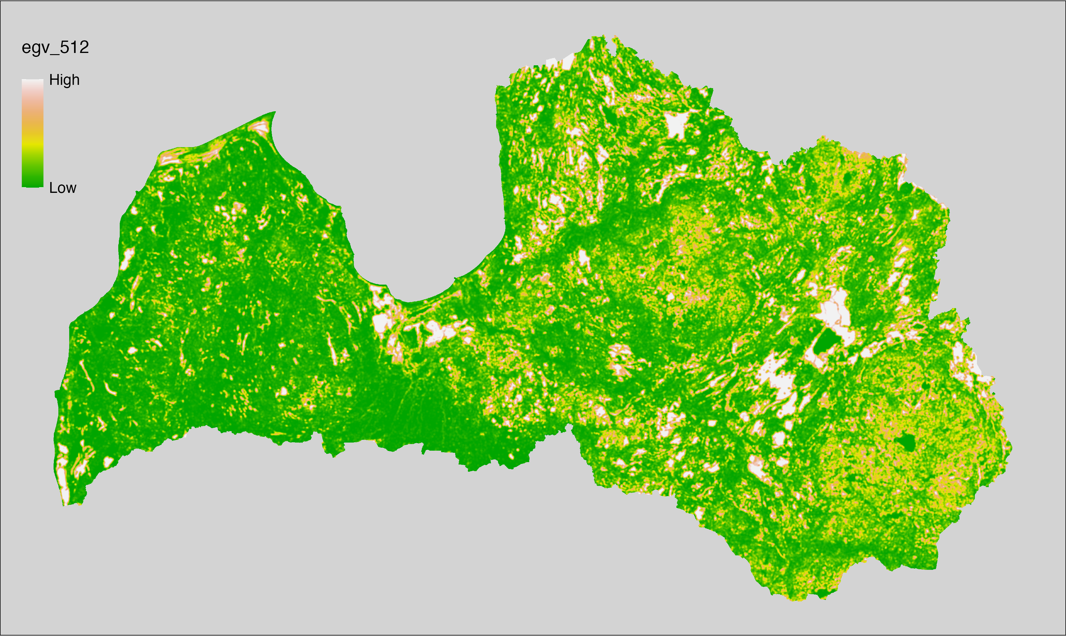
6.513 SoilTexture_Organic_r1250
filename: SoilTexture_Organic_r1250.tif
layername: egv_513
English name: Fractional cover of Organic Soils within the 1.25 km landscape
Latvian name: Augsnes granulometriskās klases “organiskās augsnes” platības īpatsvars 1,25 km ainavā
Procedure: The cover fraction within a radius of 1250 m around the analysis grid cell is
calculated as the area-weighted sum of the analysis cells inside the
buffer, using the workflow egvtools::radius_function(). During the calculation of the landscape metric,
inverse distance weighted (power = 2) gap filling on the output is applied
to ensure no missing values at the edges. Then the layer is rewritten to set
its name. Finally, the layer is standardised by subtracting the arithmetic
mean and dividing by the root mean squared error.
Code
# libs ----
if(!require(terra)) {install.packages("terra"); require(terra)}
if(!require(egvtools)) {remotes::install_github("aavotins/egvtools"); require(egvtools)}
# EGVs radii ----
radius_function(
kvadrati_path = "./Templates/TemplateGrids/tiles/",
radii_path = "./Templates/TemplateGridPoints/tiles/",
tikls100_path = "./Templates/TemplateGrids/tikls100_sauzeme.parquet",
template_path = "./Templates/TemplateRasters/LV100m_10km.tif",
input_layers = c("./RasterGrids_100m/2024/RAW/SoilTexture_Organic_cell.tif"),
layer_prefixes = c("SoilTexture_Organic"),
output_dir = "./RasterGrids_100m/2024/RAW/",
n_workers = 5,
radii = c("r1250"),
radius_mode = "sparse",
extract_fun = "mean",
fill_missing = TRUE,
IDW_weight = 2,
future_max_size = 5 * 1024^3)
# SoilTexture_Organic_r1250.tif egv_513
slanis=rast("./RasterGrids_100m/2024/RAW/SoilTexture_Organic_r1250.tif")
names(slanis)="egv_513"
slanis2=project(slanis,template100)
writeRaster(slanis2,
"./RasterGrids_100m/2024/RAW/SoilTexture_Organic_r1250.tif",
overwrite=TRUE)
# standardisation ----
if(!require(terra)) {install.packages("terra"); require(terra)}
if(!require(tidyverse)) {install.packages("tidyverse"); require(tidyverse)}
nosaukums="SoilTexture_Organic_r1250.tif"
ielasisanas_cels=paste0("./RasterGrids_100m/2024/RAW/",nosaukums)
saglabasanas_cels=paste0("./RasterGrids_100m/2024/Scaled/",nosaukums)
slanis=rast(ielasisanas_cels)
videjais=global(slanis,fun="mean",na.rm=TRUE)
centrets=slanis-videjais[,1]
standartnovirze=terra::global(centrets,fun="rms",na.rm=TRUE)
merogots=centrets/standartnovirze[,1]
writeRaster(merogots,
filename=saglabasanas_cels,
overwrite=TRUE)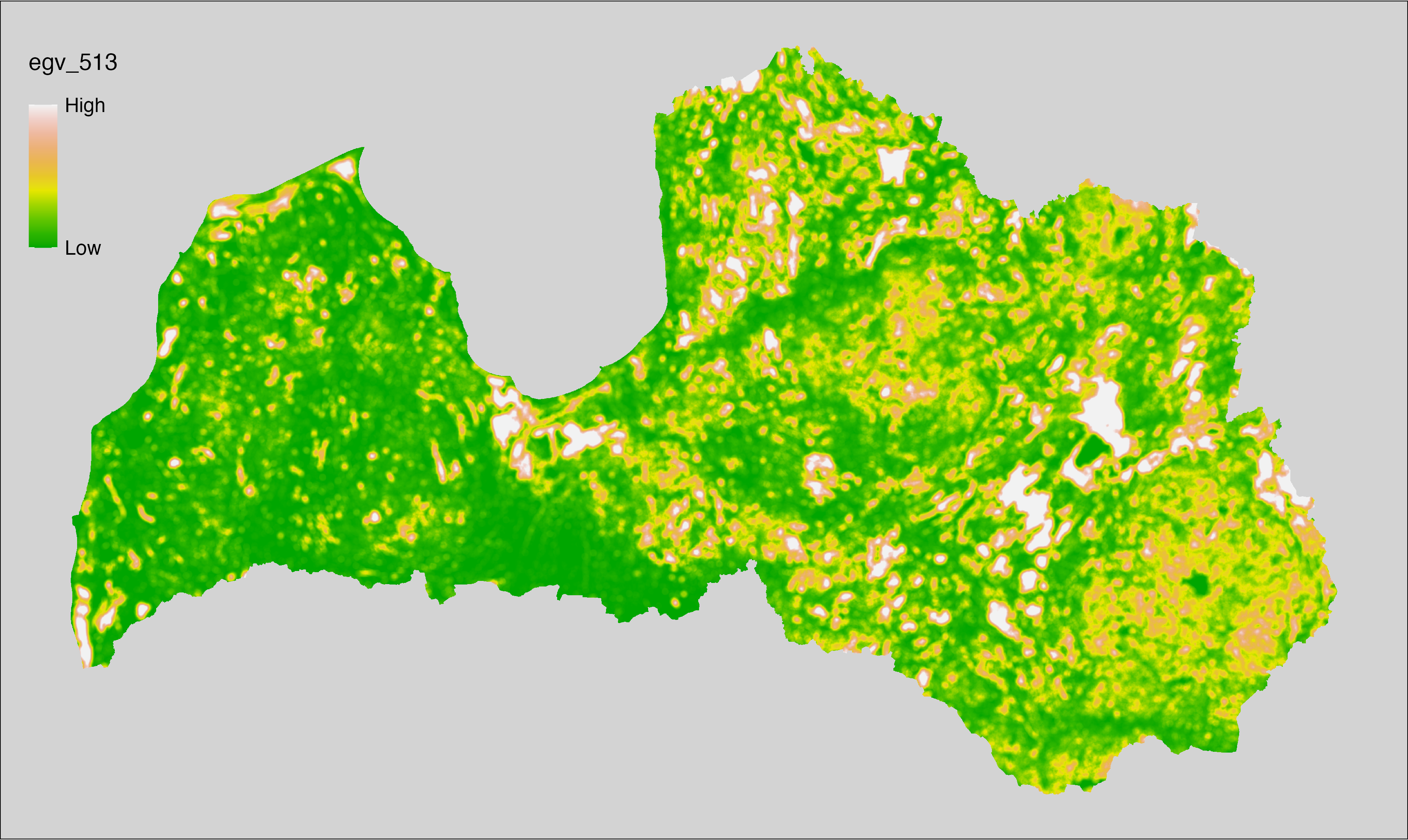
6.514 SoilTexture_Organic_r3000
filename: SoilTexture_Organic_r3000.tif
layername: egv_514
English name: Fractional cover of Organic Soils within the 3 km landscape
Latvian name: Augsnes granulometriskās klases “organiskās augsnes” platības īpatsvars 3 km ainavā
Procedure: The cover fraction within a radius of 3000 m around the analysis grid cell is
calculated as the area-weighted sum of the analysis cells inside the
buffer, using the workflow egvtools::radius_function(). During the calculation of the landscape metric,
inverse distance weighted (power = 2) gap filling on the output is applied
to ensure no missing values at the edges. Then the layer is rewritten to set
its name. Finally, the layer is standardised by subtracting the arithmetic
mean and dividing by the root mean squared error.
Code
# libs ----
if(!require(terra)) {install.packages("terra"); require(terra)}
if(!require(egvtools)) {remotes::install_github("aavotins/egvtools"); require(egvtools)}
# EGVs radii ----
radius_function(
kvadrati_path = "./Templates/TemplateGrids/tiles/",
radii_path = "./Templates/TemplateGridPoints/tiles/",
tikls100_path = "./Templates/TemplateGrids/tikls100_sauzeme.parquet",
template_path = "./Templates/TemplateRasters/LV100m_10km.tif",
input_layers = c("./RasterGrids_100m/2024/RAW/SoilTexture_Organic_cell.tif"),
layer_prefixes = c("SoilTexture_Organic"),
output_dir = "./RasterGrids_100m/2024/RAW/",
n_workers = 5,
radii = c("r3000"),
radius_mode = "sparse",
extract_fun = "mean",
fill_missing = TRUE,
IDW_weight = 2,
future_max_size = 5 * 1024^3)
# SoilTexture_Organic_r3000.tif egv_514
slanis=rast("./RasterGrids_100m/2024/RAW/SoilTexture_Organic_r3000.tif")
names(slanis)="egv_514"
slanis2=project(slanis,template100)
writeRaster(slanis2,
"./RasterGrids_100m/2024/RAW/SoilTexture_Organic_r3000.tif",
overwrite=TRUE)
# standardisation ----
if(!require(terra)) {install.packages("terra"); require(terra)}
if(!require(tidyverse)) {install.packages("tidyverse"); require(tidyverse)}
nosaukums="SoilTexture_Organic_r3000.tif"
ielasisanas_cels=paste0("./RasterGrids_100m/2024/RAW/",nosaukums)
saglabasanas_cels=paste0("./RasterGrids_100m/2024/Scaled/",nosaukums)
slanis=rast(ielasisanas_cels)
videjais=global(slanis,fun="mean",na.rm=TRUE)
centrets=slanis-videjais[,1]
standartnovirze=terra::global(centrets,fun="rms",na.rm=TRUE)
merogots=centrets/standartnovirze[,1]
writeRaster(merogots,
filename=saglabasanas_cels,
overwrite=TRUE)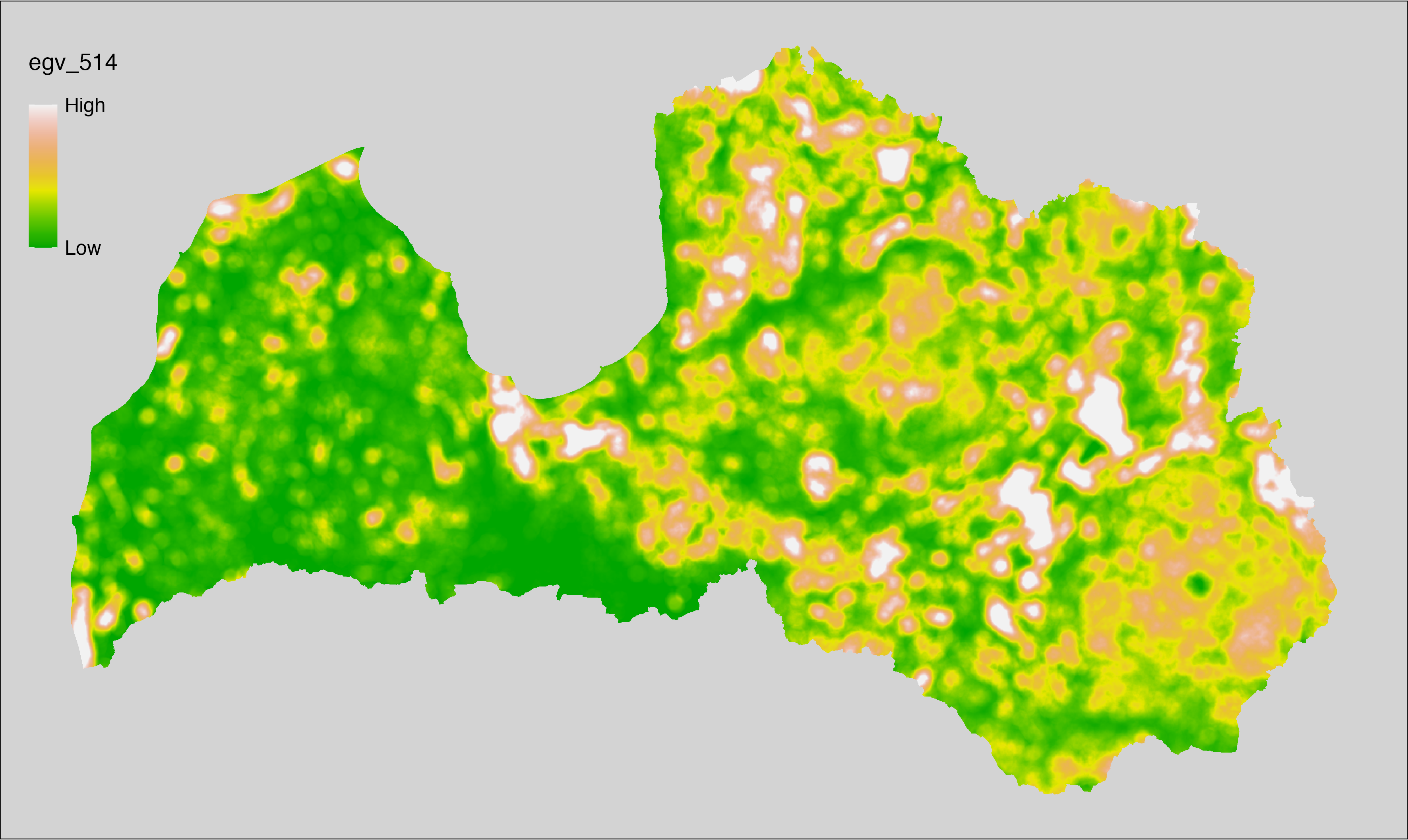
6.515 SoilTexture_Organic_r10000
filename: SoilTexture_Organic_r10000.tif
layername: egv_515
English name: Fractional cover of Organic Soils within the 10 km landscape
Latvian name: Augsnes granulometriskās klases “organiskās augsnes” platības īpatsvars 10 km ainavā
Procedure: The cover fraction within a radius of 10000 m around the analysis grid cell is
calculated as the area-weighted sum of the analysis cells inside the
buffer, using the workflow egvtools::radius_function(). During the calculation of the landscape metric,
inverse distance weighted (power = 2) gap filling on the output is applied
to ensure no missing values at the edges. Then the layer is rewritten to set
its name. Finally, the layer is standardised by subtracting the arithmetic
mean and dividing by the root mean squared error.
Code
# libs ----
if(!require(terra)) {install.packages("terra"); require(terra)}
if(!require(egvtools)) {remotes::install_github("aavotins/egvtools"); require(egvtools)}
# EGVs radii ----
radius_function(
kvadrati_path = "./Templates/TemplateGrids/tiles/",
radii_path = "./Templates/TemplateGridPoints/tiles/",
tikls100_path = "./Templates/TemplateGrids/tikls100_sauzeme.parquet",
template_path = "./Templates/TemplateRasters/LV100m_10km.tif",
input_layers = c("./RasterGrids_100m/2024/RAW/SoilTexture_Organic_cell.tif"),
layer_prefixes = c("SoilTexture_Organic"),
output_dir = "./RasterGrids_100m/2024/RAW/",
n_workers = 5,
radii = c("r10000"),
radius_mode = "sparse",
extract_fun = "mean",
fill_missing = TRUE,
IDW_weight = 2,
future_max_size = 5 * 1024^3)
# SoilTexture_Organic_r10000.tif egv_515
slanis=rast("./RasterGrids_100m/2024/RAW/SoilTexture_Organic_r10000.tif")
names(slanis)="egv_515"
slanis2=project(slanis,template100)
writeRaster(slanis2,
"./RasterGrids_100m/2024/RAW/SoilTexture_Organic_r10000.tif",
overwrite=TRUE)
# standardisation ----
if(!require(terra)) {install.packages("terra"); require(terra)}
if(!require(tidyverse)) {install.packages("tidyverse"); require(tidyverse)}
nosaukums="SoilTexture_Organic_r10000.tif"
ielasisanas_cels=paste0("./RasterGrids_100m/2024/RAW/",nosaukums)
saglabasanas_cels=paste0("./RasterGrids_100m/2024/Scaled/",nosaukums)
slanis=rast(ielasisanas_cels)
videjais=global(slanis,fun="mean",na.rm=TRUE)
centrets=slanis-videjais[,1]
standartnovirze=terra::global(centrets,fun="rms",na.rm=TRUE)
merogots=centrets/standartnovirze[,1]
writeRaster(merogots,
filename=saglabasanas_cels,
overwrite=TRUE)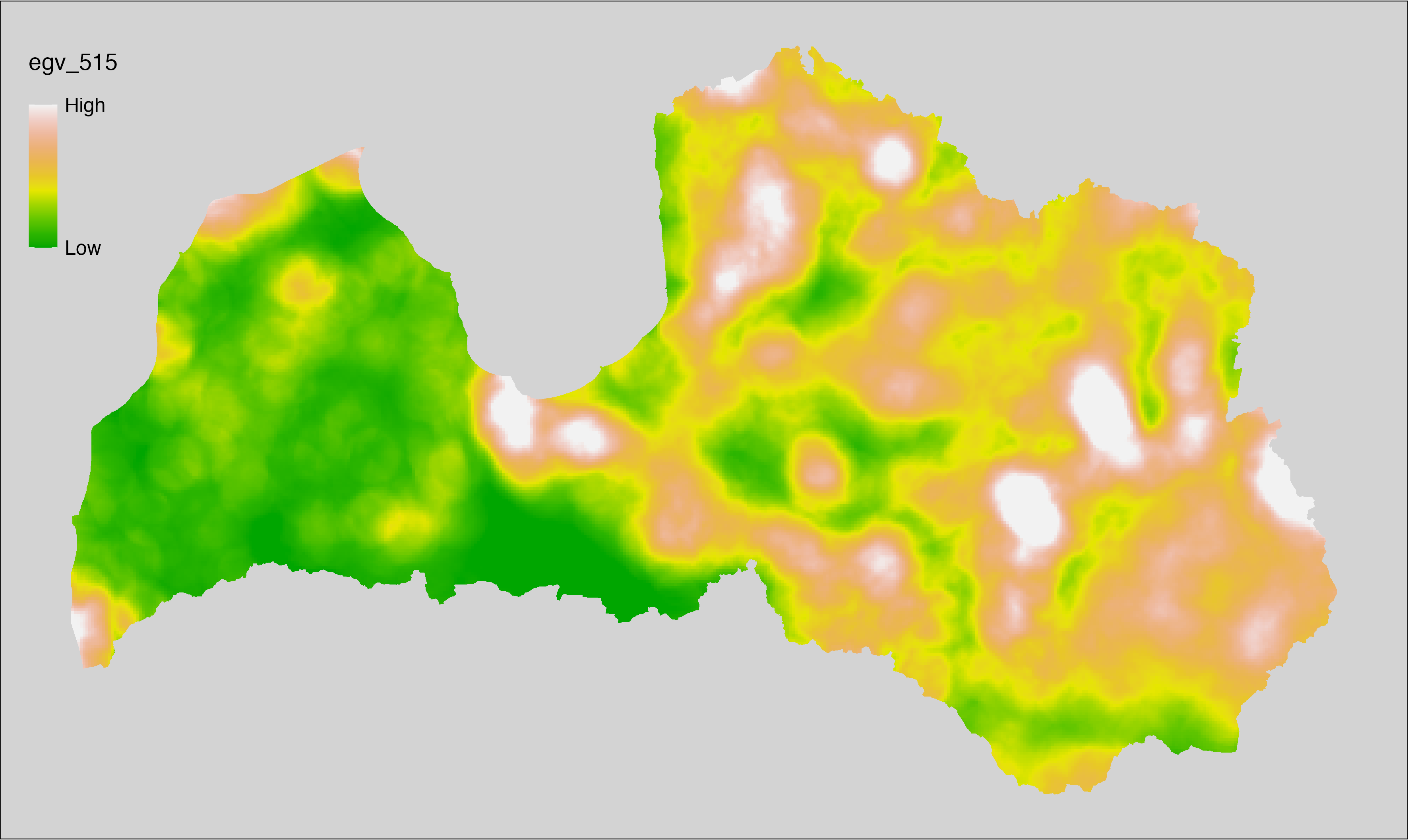
6.516 SoilTexture_Sand_cell
filename: SoilTexture_Sand_cell.tif
layername: egv_516
English name: Fractional cover of Sand Soils within the analysis cell (1 ha)
Latvian name: Augsnes granulometriskās klases “smilts” platības īpatsvars analīzes šūnā (1 ha)
Procedure: Derived from the Soil texture product. First, the layer is
reclassified so that the class of interest is 1 and the other classes are 0. The resulting layer
is then aggregated to EGV resolution using the workflow egvtools::input2egv(), which
calculates the arithmetic mean to determine the cover fraction. During
aggregation, inverse distance weighted (power = 2) gap filling on the output is
applied to ensure no missing values at the edges. Finally, the layer is
standardised by subtracting the arithmetic mean and dividing by the root mean squared
error.
Code
# libs ----
if(!require(terra)) {install.packages("terra"); require(terra)}
if(!require(egvtools)) {remotes::install_github("aavotins/egvtools"); require(egvtools)}
# templates ----
template10=rast("./Templates/TemplateRasters/LV10m_10km.tif")
template100=rast("./Templates/TemplateRasters/LV100m_10km.tif")
# input ----
combtext=rast("./RasterGrids_10m/2024/SoilTXT_combined.tif")
# EGVs cell ----
# SoilTexture_Sand_cell.tif egv_516
sand10=ifel(combtext==1,1,0)
plot(sand10)
input2egv(input=sand10,
egv_template="./Templates/TemplateRasters/LV100m_10km.tif",
summary_function = "average",
missing_job = "FillOutput",
idw_weight = 2,
outlocation = "./RasterGrids_100m/2024/RAW/",
outfilename = "SoilTexture_Sand_cell.tif",
layername="egv_516",
return_visible = TRUE)
# standardisation ----
if(!require(terra)) {install.packages("terra"); require(terra)}
if(!require(tidyverse)) {install.packages("tidyverse"); require(tidyverse)}
nosaukums="SoilTexture_Sand_cell.tif"
ielasisanas_cels=paste0("./RasterGrids_100m/2024/RAW/",nosaukums)
saglabasanas_cels=paste0("./RasterGrids_100m/2024/Scaled/",nosaukums)
slanis=rast(ielasisanas_cels)
videjais=global(slanis,fun="mean",na.rm=TRUE)
centrets=slanis-videjais[,1]
standartnovirze=terra::global(centrets,fun="rms",na.rm=TRUE)
merogots=centrets/standartnovirze[,1]
writeRaster(merogots,
filename=saglabasanas_cels,
overwrite=TRUE)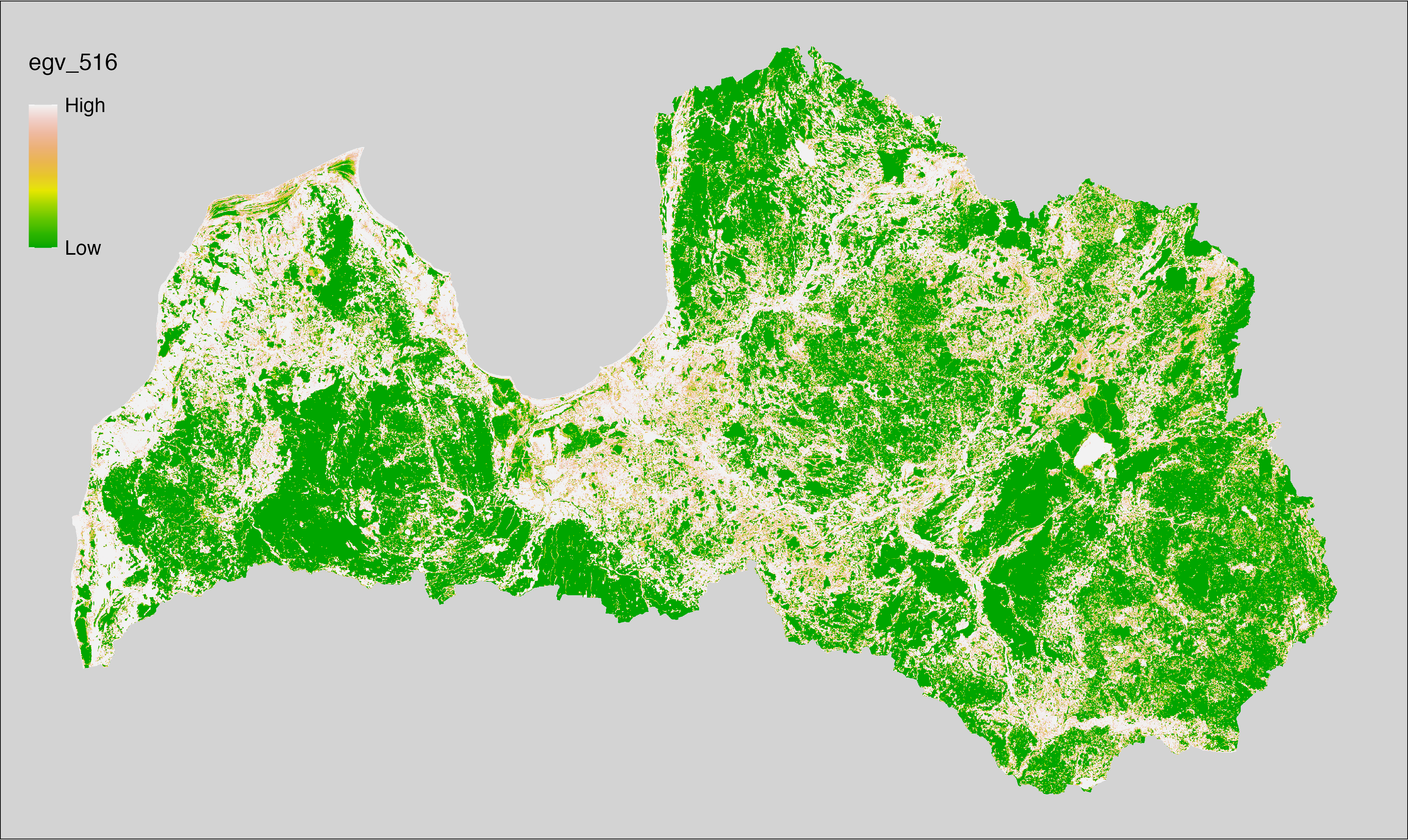
6.517 SoilTexture_Sand_r500
filename: SoilTexture_Sand_r500.tif
layername: egv_517
English name: Fractional cover of Sand Soils within the 0.5 km landscape
Latvian name: Augsnes granulometriskās klases “smilts” platības īpatsvars 0,5 km ainavā
Procedure: The cover fraction within a radius of 500 m around the analysis grid cell is
calculated as the area-weighted sum of the analysis cells inside the
buffer, using the workflow egvtools::radius_function(). During the calculation of the landscape metric,
inverse distance weighted (power = 2) gap filling on the output is applied
to ensure no missing values at the edges. Then the layer is rewritten to set
its name. Finally, the layer is standardised by subtracting the arithmetic
mean and dividing by the root mean squared error.
Code
# libs ----
if(!require(terra)) {install.packages("terra"); require(terra)}
if(!require(egvtools)) {remotes::install_github("aavotins/egvtools"); require(egvtools)}
# EGVs radii ----
radius_function(
kvadrati_path = "./Templates/TemplateGrids/tiles/",
radii_path = "./Templates/TemplateGridPoints/tiles/",
tikls100_path = "./Templates/TemplateGrids/tikls100_sauzeme.parquet",
template_path = "./Templates/TemplateRasters/LV100m_10km.tif",
input_layers = c("./RasterGrids_100m/2024/RAW/SoilTexture_Sand_cell.tif"),
layer_prefixes = c("SoilTexture_Sand"),
output_dir = "./RasterGrids_100m/2024/RAW/",
n_workers = 5,
radii = c("r500"),
radius_mode = "sparse",
extract_fun = "mean",
fill_missing = TRUE,
IDW_weight = 2,
future_max_size = 5 * 1024^3)
# SoilTexture_Sand_r500.tif egv_517
slanis=rast("./RasterGrids_100m/2024/RAW/SoilTexture_Sand_r500.tif")
names(slanis)="egv_517"
slanis2=project(slanis,template100)
writeRaster(slanis2,
"./RasterGrids_100m/2024/RAW/SoilTexture_Sand_r500.tif",
overwrite=TRUE)
# standardisation ----
if(!require(terra)) {install.packages("terra"); require(terra)}
if(!require(tidyverse)) {install.packages("tidyverse"); require(tidyverse)}
nosaukums="SoilTexture_Sand_r500.tif"
ielasisanas_cels=paste0("./RasterGrids_100m/2024/RAW/",nosaukums)
saglabasanas_cels=paste0("./RasterGrids_100m/2024/Scaled/",nosaukums)
slanis=rast(ielasisanas_cels)
videjais=global(slanis,fun="mean",na.rm=TRUE)
centrets=slanis-videjais[,1]
standartnovirze=terra::global(centrets,fun="rms",na.rm=TRUE)
merogots=centrets/standartnovirze[,1]
writeRaster(merogots,
filename=saglabasanas_cels,
overwrite=TRUE)
6.518 SoilTexture_Sand_r1250
filename: SoilTexture_Sand_r1250.tif
layername: egv_518
English name: Fractional cover of Sand Soils within the 1.25 km landscape
Latvian name: Augsnes granulometriskās klases “smilts” platības īpatsvars 1,25 km ainavā
Procedure: The cover fraction within a radius of 1250 m around the analysis grid cell is
calculated as the area-weighted sum of the analysis cells inside the
buffer, using the workflow egvtools::radius_function(). During the calculation of the landscape metric,
inverse distance weighted (power = 2) gap filling on the output is applied
to ensure no missing values at the edges. Then the layer is rewritten to set
its name. Finally, the layer is standardised by subtracting the arithmetic
mean and dividing by the root mean squared error.
Code
# libs ----
if(!require(terra)) {install.packages("terra"); require(terra)}
if(!require(egvtools)) {remotes::install_github("aavotins/egvtools"); require(egvtools)}
# EGVs radii ----
radius_function(
kvadrati_path = "./Templates/TemplateGrids/tiles/",
radii_path = "./Templates/TemplateGridPoints/tiles/",
tikls100_path = "./Templates/TemplateGrids/tikls100_sauzeme.parquet",
template_path = "./Templates/TemplateRasters/LV100m_10km.tif",
input_layers = c("./RasterGrids_100m/2024/RAW/SoilTexture_Sand_cell.tif"),
layer_prefixes = c("SoilTexture_Sand"),
output_dir = "./RasterGrids_100m/2024/RAW/",
n_workers = 5,
radii = c("r1250"),
radius_mode = "sparse",
extract_fun = "mean",
fill_missing = TRUE,
IDW_weight = 2,
future_max_size = 5 * 1024^3)
# SoilTexture_Sand_r1250.tif egv_518
slanis=rast("./RasterGrids_100m/2024/RAW/SoilTexture_Sand_r1250.tif")
names(slanis)="egv_518"
slanis2=project(slanis,template100)
writeRaster(slanis2,
"./RasterGrids_100m/2024/RAW/SoilTexture_Sand_r1250.tif",
overwrite=TRUE)
# standardisation ----
if(!require(terra)) {install.packages("terra"); require(terra)}
if(!require(tidyverse)) {install.packages("tidyverse"); require(tidyverse)}
nosaukums="SoilTexture_Sand_r1250.tif"
ielasisanas_cels=paste0("./RasterGrids_100m/2024/RAW/",nosaukums)
saglabasanas_cels=paste0("./RasterGrids_100m/2024/Scaled/",nosaukums)
slanis=rast(ielasisanas_cels)
videjais=global(slanis,fun="mean",na.rm=TRUE)
centrets=slanis-videjais[,1]
standartnovirze=terra::global(centrets,fun="rms",na.rm=TRUE)
merogots=centrets/standartnovirze[,1]
writeRaster(merogots,
filename=saglabasanas_cels,
overwrite=TRUE)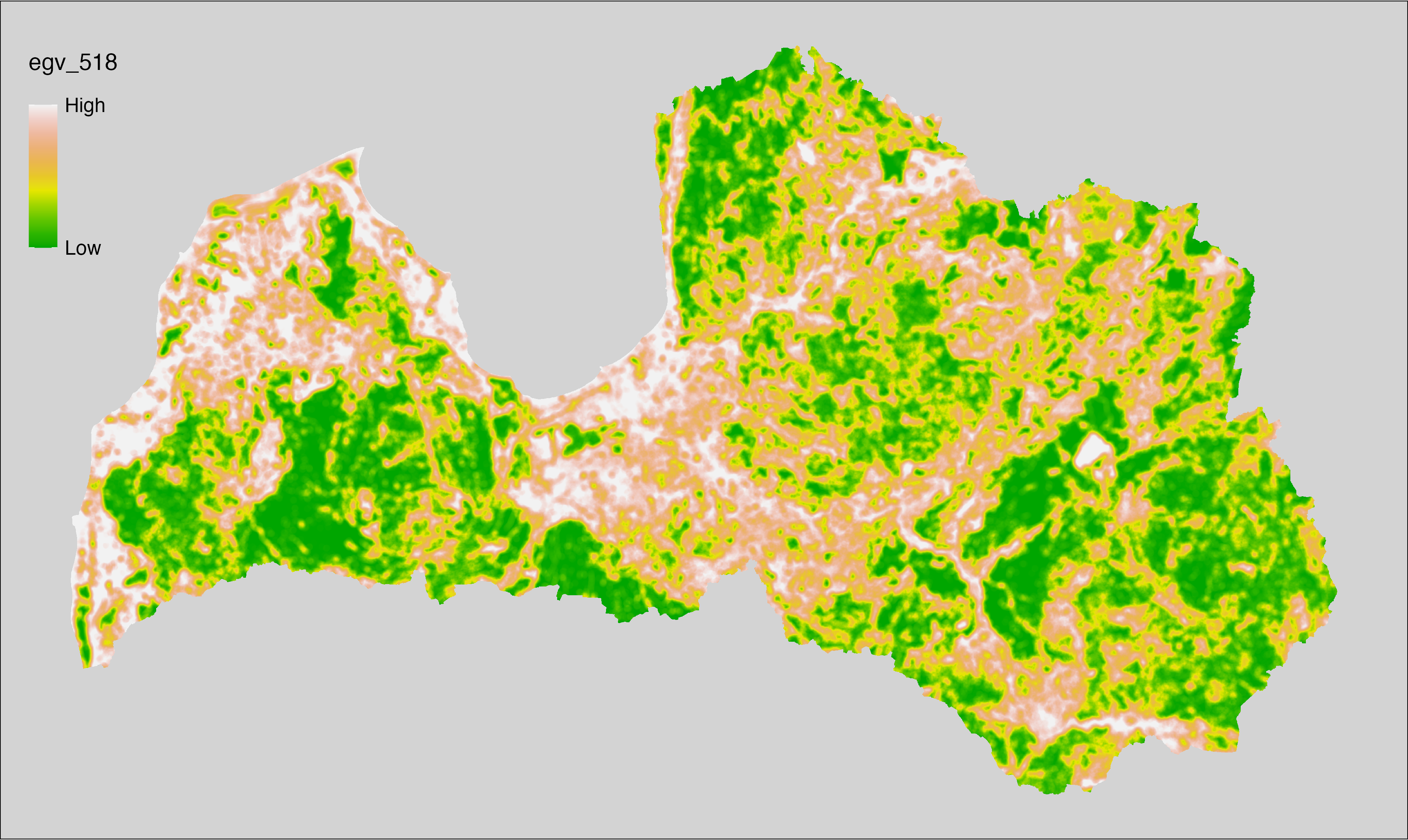
6.519 SoilTexture_Sand_r3000
filename: SoilTexture_Sand_r3000.tif
layername: egv_519
English name: Fractional cover of Sand Soils within the 3 km landscape
Latvian name: Augsnes granulometriskās klases “smilts” platības īpatsvars 3 km ainavā
Procedure: The cover fraction within a radius of 3000 m around the analysis grid cell is
calculated as the area-weighted sum of the analysis cells inside the
buffer, using the workflow egvtools::radius_function(). During the calculation of the landscape metric,
inverse distance weighted (power = 2) gap filling on the output is applied
to ensure no missing values at the edges. Then the layer is rewritten to set
its name. Finally, the layer is standardised by subtracting the arithmetic
mean and dividing by the root mean squared error.
Code
# libs ----
if(!require(terra)) {install.packages("terra"); require(terra)}
if(!require(egvtools)) {remotes::install_github("aavotins/egvtools"); require(egvtools)}
# EGVs radii ----
radius_function(
kvadrati_path = "./Templates/TemplateGrids/tiles/",
radii_path = "./Templates/TemplateGridPoints/tiles/",
tikls100_path = "./Templates/TemplateGrids/tikls100_sauzeme.parquet",
template_path = "./Templates/TemplateRasters/LV100m_10km.tif",
input_layers = c("./RasterGrids_100m/2024/RAW/SoilTexture_Sand_cell.tif"),
layer_prefixes = c("SoilTexture_Sand"),
output_dir = "./RasterGrids_100m/2024/RAW/",
n_workers = 5,
radii = c("r3000"),
radius_mode = "sparse",
extract_fun = "mean",
fill_missing = TRUE,
IDW_weight = 2,
future_max_size = 5 * 1024^3)
# SoilTexture_Sand_r3000.tif egv_519
slanis=rast("./RasterGrids_100m/2024/RAW/SoilTexture_Sand_r3000.tif")
names(slanis)="egv_519"
slanis2=project(slanis,template100)
writeRaster(slanis2,
"./RasterGrids_100m/2024/RAW/SoilTexture_Sand_r3000.tif",
overwrite=TRUE)
# standardisation ----
if(!require(terra)) {install.packages("terra"); require(terra)}
if(!require(tidyverse)) {install.packages("tidyverse"); require(tidyverse)}
nosaukums="SoilTexture_Sand_r3000.tif"
ielasisanas_cels=paste0("./RasterGrids_100m/2024/RAW/",nosaukums)
saglabasanas_cels=paste0("./RasterGrids_100m/2024/Scaled/",nosaukums)
slanis=rast(ielasisanas_cels)
videjais=global(slanis,fun="mean",na.rm=TRUE)
centrets=slanis-videjais[,1]
standartnovirze=terra::global(centrets,fun="rms",na.rm=TRUE)
merogots=centrets/standartnovirze[,1]
writeRaster(merogots,
filename=saglabasanas_cels,
overwrite=TRUE)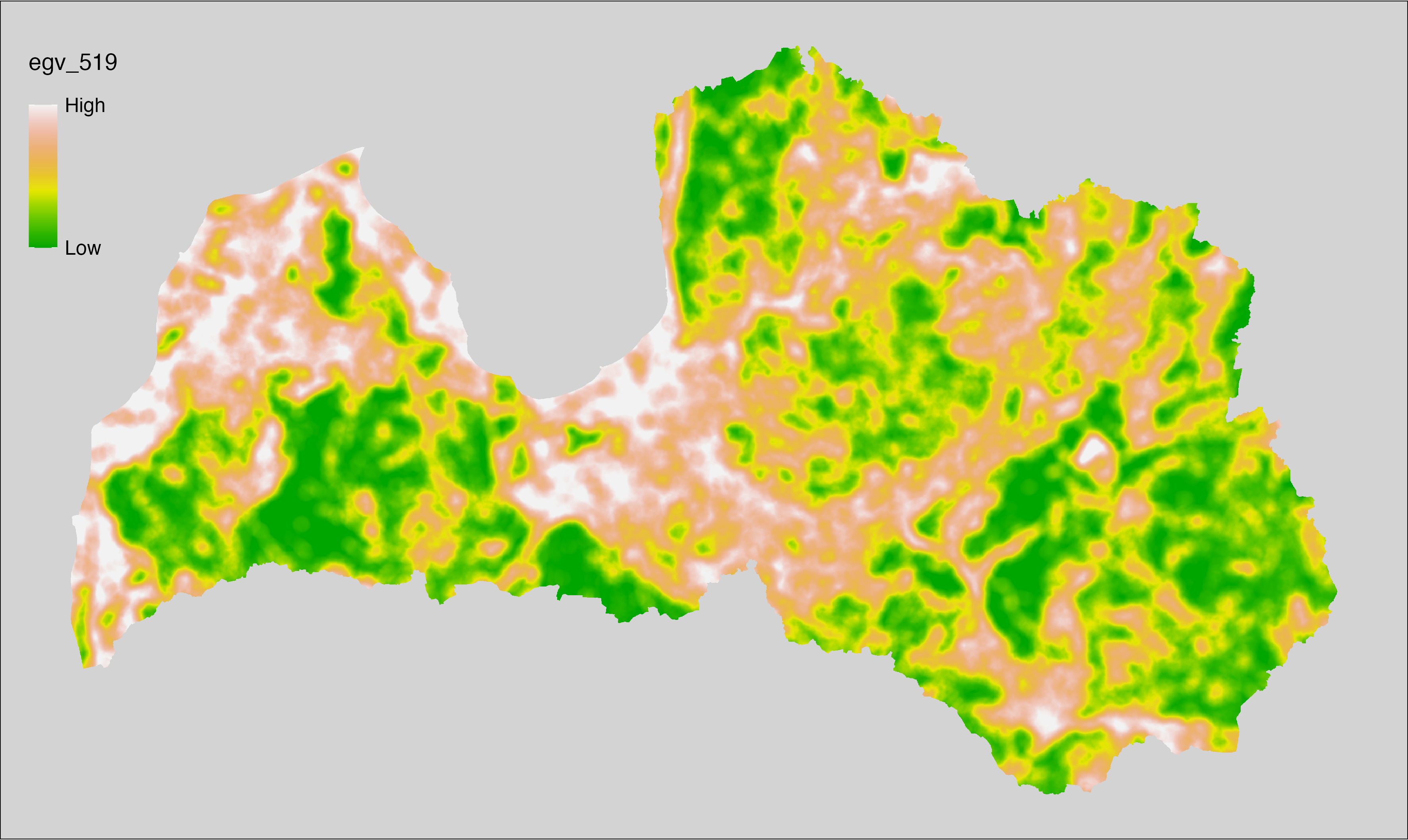
6.520 SoilTexture_Sand_r10000
filename: SoilTexture_Sand_r10000.tif
layername: egv_520
English name: Fractional cover of Sand Soils within the 10 km landscape
Latvian name: Augsnes granulometriskās klases “smilts” platības īpatsvars 10 km ainavā
Procedure: The cover fraction within a radius of 10000 m around the analysis grid cell is
calculated as the area-weighted sum of the analysis cells inside the
buffer, using the workflow egvtools::radius_function(). During the calculation of the landscape metric,
inverse distance weighted (power = 2) gap filling on the output is applied
to ensure no missing values at the edges. Then the layer is rewritten to set
its name. Finally, the layer is standardised by subtracting the arithmetic
mean and dividing by the root mean squared error.
Code
# libs ----
if(!require(terra)) {install.packages("terra"); require(terra)}
if(!require(egvtools)) {remotes::install_github("aavotins/egvtools"); require(egvtools)}
# EGVs radii ----
radius_function(
kvadrati_path = "./Templates/TemplateGrids/tiles/",
radii_path = "./Templates/TemplateGridPoints/tiles/",
tikls100_path = "./Templates/TemplateGrids/tikls100_sauzeme.parquet",
template_path = "./Templates/TemplateRasters/LV100m_10km.tif",
input_layers = c("./RasterGrids_100m/2024/RAW/SoilTexture_Sand_cell.tif"),
layer_prefixes = c("SoilTexture_Sand"),
output_dir = "./RasterGrids_100m/2024/RAW/",
n_workers = 5,
radii = c("r10000"),
radius_mode = "sparse",
extract_fun = "mean",
fill_missing = TRUE,
IDW_weight = 2,
future_max_size = 5 * 1024^3)
# SoilTexture_Sand_r10000.tif egv_520
slanis=rast("./RasterGrids_100m/2024/RAW/SoilTexture_Sand_r10000.tif")
names(slanis)="egv_520"
slanis2=project(slanis,template100)
writeRaster(slanis2,
"./RasterGrids_100m/2024/RAW/SoilTexture_Sand_r10000.tif",
overwrite=TRUE)
# standardisation ----
if(!require(terra)) {install.packages("terra"); require(terra)}
if(!require(tidyverse)) {install.packages("tidyverse"); require(tidyverse)}
nosaukums="SoilTexture_Sand_r10000.tif"
ielasisanas_cels=paste0("./RasterGrids_100m/2024/RAW/",nosaukums)
saglabasanas_cels=paste0("./RasterGrids_100m/2024/Scaled/",nosaukums)
slanis=rast(ielasisanas_cels)
videjais=global(slanis,fun="mean",na.rm=TRUE)
centrets=slanis-videjais[,1]
standartnovirze=terra::global(centrets,fun="rms",na.rm=TRUE)
merogots=centrets/standartnovirze[,1]
writeRaster(merogots,
filename=saglabasanas_cels,
overwrite=TRUE)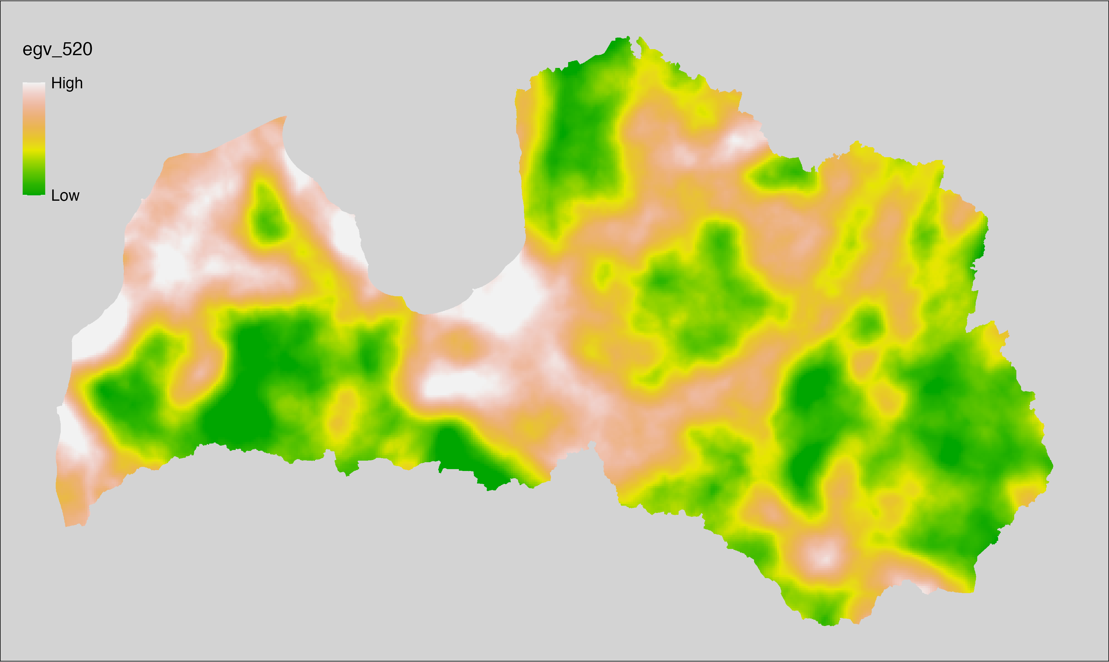
6.521 SoilTexture_Silt_cell
filename: SoilTexture_Silt_cell.tif
layername: egv_521
English name: Fractional cover of Silt Soils within the analysis cell (1 ha)
Latvian name: Augsnes granulometriskās klases “smilšmāls un mālsmilts” platības īpatsvars analīzes šūnā (1 ha)
Procedure: Derived from the Soil texture product. First, the layer is
reclassified so that the class of interest is 1 and the other classes are 0. The resulting layer
is then aggregated to EGV resolution using the workflow egvtools::input2egv(), which
calculates the arithmetic mean to determine the cover fraction. During
aggregation, inverse distance weighted (power = 2) gap filling on the output is
applied to ensure no missing values at the edges. Finally, the layer is
standardised by subtracting the arithmetic mean and dividing by the root mean squared
error.
Code
# libs ----
if(!require(terra)) {install.packages("terra"); require(terra)}
if(!require(egvtools)) {remotes::install_github("aavotins/egvtools"); require(egvtools)}
# templates ----
template10=rast("./Templates/TemplateRasters/LV10m_10km.tif")
template100=rast("./Templates/TemplateRasters/LV100m_10km.tif")
# input ----
combtext=rast("./RasterGrids_10m/2024/SoilTXT_combined.tif")
# EGVs cell ----
# SoilTexture_Silt_cell.tif egv_521
silt10=ifel(combtext==2,1,0)
input2egv(input=silt10,
egv_template="./Templates/TemplateRasters/LV100m_10km.tif",
summary_function = "average",
missing_job = "FillOutput",
idw_weight = 2,
outlocation = "./RasterGrids_100m/2024/RAW/",
outfilename = "SoilTexture_Silt_cell.tif",
layername="egv_521",
return_visible = TRUE)
# standardisation ----
if(!require(terra)) {install.packages("terra"); require(terra)}
if(!require(tidyverse)) {install.packages("tidyverse"); require(tidyverse)}
nosaukums="SoilTexture_Silt_cell.tif"
ielasisanas_cels=paste0("./RasterGrids_100m/2024/RAW/",nosaukums)
saglabasanas_cels=paste0("./RasterGrids_100m/2024/Scaled/",nosaukums)
slanis=rast(ielasisanas_cels)
videjais=global(slanis,fun="mean",na.rm=TRUE)
centrets=slanis-videjais[,1]
standartnovirze=terra::global(centrets,fun="rms",na.rm=TRUE)
merogots=centrets/standartnovirze[,1]
writeRaster(merogots,
filename=saglabasanas_cels,
overwrite=TRUE)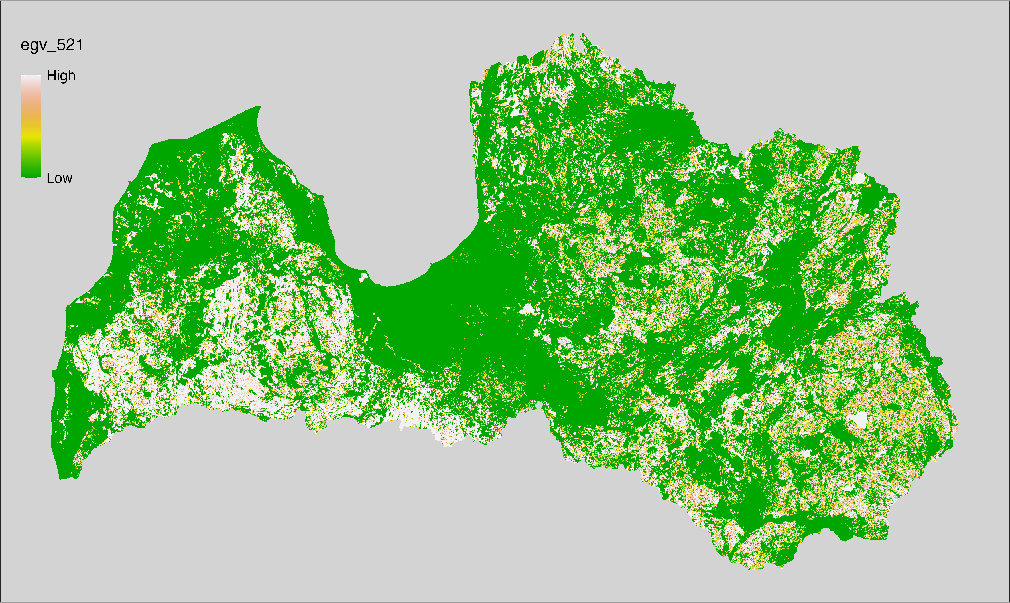
6.522 SoilTexture_Silt_r500
filename: SoilTexture_Silt_r500.tif
layername: egv_522
English name: Fractional cover of Silt Soils within the 0.5 km landscape
Latvian name: Augsnes granulometriskās klases “smilšmāls un mālsmilts” platības īpatsvars 0,5 km ainavā
Procedure: The cover fraction within a radius of 500 m around the analysis grid cell is
calculated as the area-weighted sum of the analysis cells inside the
buffer, using the workflow egvtools::radius_function(). During the calculation of the landscape metric,
inverse distance weighted (power = 2) gap filling on the output is applied
to ensure no missing values at the edges. Then the layer is rewritten to set
its name. Finally, the layer is standardised by subtracting the arithmetic
mean and dividing by the root mean squared error.
Code
# libs ----
if(!require(terra)) {install.packages("terra"); require(terra)}
if(!require(egvtools)) {remotes::install_github("aavotins/egvtools"); require(egvtools)}
# EGVs radii ----
radius_function(
kvadrati_path = "./Templates/TemplateGrids/tiles/",
radii_path = "./Templates/TemplateGridPoints/tiles/",
tikls100_path = "./Templates/TemplateGrids/tikls100_sauzeme.parquet",
template_path = "./Templates/TemplateRasters/LV100m_10km.tif",
input_layers = c("./RasterGrids_100m/2024/RAW/SoilTexture_Silt_cell.tif"),
layer_prefixes = c("SoilTexture_Silt"),
output_dir = "./RasterGrids_100m/2024/RAW/",
n_workers = 5,
radii = c("r500"),
radius_mode = "sparse",
extract_fun = "mean",
fill_missing = TRUE,
IDW_weight = 2,
future_max_size = 5 * 1024^3)
# SoilTexture_Silt_r500.tif egv_522
slanis=rast("./RasterGrids_100m/2024/RAW/SoilTexture_Silt_r500.tif")
names(slanis)="egv_522"
slanis2=project(slanis,template100)
writeRaster(slanis2,
"./RasterGrids_100m/2024/RAW/SoilTexture_Silt_r500.tif",
overwrite=TRUE)
# standardisation ----
if(!require(terra)) {install.packages("terra"); require(terra)}
if(!require(tidyverse)) {install.packages("tidyverse"); require(tidyverse)}
nosaukums="SoilTexture_Silt_r500.tif"
ielasisanas_cels=paste0("./RasterGrids_100m/2024/RAW/",nosaukums)
saglabasanas_cels=paste0("./RasterGrids_100m/2024/Scaled/",nosaukums)
slanis=rast(ielasisanas_cels)
videjais=global(slanis,fun="mean",na.rm=TRUE)
centrets=slanis-videjais[,1]
standartnovirze=terra::global(centrets,fun="rms",na.rm=TRUE)
merogots=centrets/standartnovirze[,1]
writeRaster(merogots,
filename=saglabasanas_cels,
overwrite=TRUE)
6.523 SoilTexture_Silt_r1250
filename: SoilTexture_Silt_r1250.tif
layername: egv_523
English name: Fractional cover of Silt Soils within the 1.25 km landscape
Latvian name: Augsnes granulometriskās klases “smilšmāls un mālsmilts” platības īpatsvars 1,25 km ainavā
Procedure: The cover fraction within a radius of 1250 m around the analysis grid cell is
calculated as the area-weighted sum of the analysis cells inside the
buffer, using the workflow egvtools::radius_function(). During the calculation of the landscape metric,
inverse distance weighted (power = 2) gap filling on the output is applied
to ensure no missing values at the edges. Then the layer is rewritten to set
its name. Finally, the layer is standardised by subtracting the arithmetic
mean and dividing by the root mean squared error.
Code
# libs ----
if(!require(terra)) {install.packages("terra"); require(terra)}
if(!require(egvtools)) {remotes::install_github("aavotins/egvtools"); require(egvtools)}
# EGVs radii ----
radius_function(
kvadrati_path = "./Templates/TemplateGrids/tiles/",
radii_path = "./Templates/TemplateGridPoints/tiles/",
tikls100_path = "./Templates/TemplateGrids/tikls100_sauzeme.parquet",
template_path = "./Templates/TemplateRasters/LV100m_10km.tif",
input_layers = c("./RasterGrids_100m/2024/RAW/SoilTexture_Silt_cell.tif"),
layer_prefixes = c("SoilTexture_Silt"),
output_dir = "./RasterGrids_100m/2024/RAW/",
n_workers = 5,
radii = c("r1250"),
radius_mode = "sparse",
extract_fun = "mean",
fill_missing = TRUE,
IDW_weight = 2,
future_max_size = 5 * 1024^3)
# SoilTexture_Silt_r1250.tif egv_523
slanis=rast("./RasterGrids_100m/2024/RAW/SoilTexture_Silt_r1250.tif")
names(slanis)="egv_523"
slanis2=project(slanis,template100)
writeRaster(slanis2,
"./RasterGrids_100m/2024/RAW/SoilTexture_Silt_r1250.tif",
overwrite=TRUE)
# standardisation ----
if(!require(terra)) {install.packages("terra"); require(terra)}
if(!require(tidyverse)) {install.packages("tidyverse"); require(tidyverse)}
nosaukums="SoilTexture_Silt_r1250.tif"
ielasisanas_cels=paste0("./RasterGrids_100m/2024/RAW/",nosaukums)
saglabasanas_cels=paste0("./RasterGrids_100m/2024/Scaled/",nosaukums)
slanis=rast(ielasisanas_cels)
videjais=global(slanis,fun="mean",na.rm=TRUE)
centrets=slanis-videjais[,1]
standartnovirze=terra::global(centrets,fun="rms",na.rm=TRUE)
merogots=centrets/standartnovirze[,1]
writeRaster(merogots,
filename=saglabasanas_cels,
overwrite=TRUE)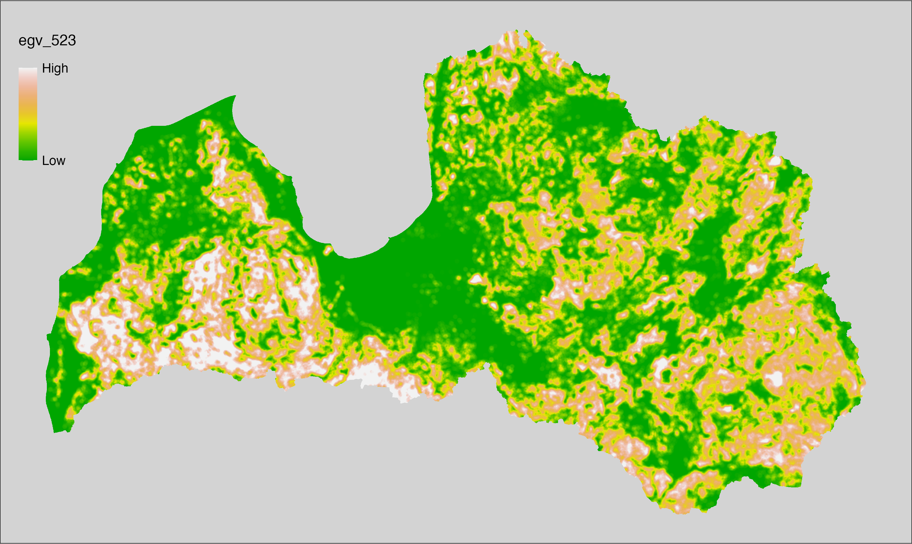
6.524 SoilTexture_Silt_r3000
filename: SoilTexture_Silt_r3000.tif
layername: egv_524
English name: Fractional cover of Silt Soils within the 3 km landscape
Latvian name: Augsnes granulometriskās klases “smilšmāls un mālsmilts” platības īpatsvars 3 km ainavā
Procedure: The cover fraction within a radius of 3000 m around the analysis grid cell is
calculated as the area-weighted sum of the analysis cells inside the
buffer, using the workflow egvtools::radius_function(). During the calculation of the landscape metric,
inverse distance weighted (power = 2) gap filling on the output is applied
to ensure no missing values at the edges. Then the layer is rewritten to set
its name. Finally, the layer is standardised by subtracting the arithmetic
mean and dividing by the root mean squared error.
Code
# libs ----
if(!require(terra)) {install.packages("terra"); require(terra)}
if(!require(egvtools)) {remotes::install_github("aavotins/egvtools"); require(egvtools)}
# EGVs radii ----
radius_function(
kvadrati_path = "./Templates/TemplateGrids/tiles/",
radii_path = "./Templates/TemplateGridPoints/tiles/",
tikls100_path = "./Templates/TemplateGrids/tikls100_sauzeme.parquet",
template_path = "./Templates/TemplateRasters/LV100m_10km.tif",
input_layers = c("./RasterGrids_100m/2024/RAW/SoilTexture_Silt_cell.tif"),
layer_prefixes = c("SoilTexture_Silt"),
output_dir = "./RasterGrids_100m/2024/RAW/",
n_workers = 5,
radii = c("r3000"),
radius_mode = "sparse",
extract_fun = "mean",
fill_missing = TRUE,
IDW_weight = 2,
future_max_size = 5 * 1024^3)
# SoilTexture_Silt_r3000.tif egv_524
slanis=rast("./RasterGrids_100m/2024/RAW/SoilTexture_Silt_r3000.tif")
names(slanis)="egv_524"
slanis2=project(slanis,template100)
writeRaster(slanis2,
"./RasterGrids_100m/2024/RAW/SoilTexture_Silt_r3000.tif",
overwrite=TRUE)
# standardisation ----
if(!require(terra)) {install.packages("terra"); require(terra)}
if(!require(tidyverse)) {install.packages("tidyverse"); require(tidyverse)}
nosaukums="SoilTexture_Silt_r3000.tif"
ielasisanas_cels=paste0("./RasterGrids_100m/2024/RAW/",nosaukums)
saglabasanas_cels=paste0("./RasterGrids_100m/2024/Scaled/",nosaukums)
slanis=rast(ielasisanas_cels)
videjais=global(slanis,fun="mean",na.rm=TRUE)
centrets=slanis-videjais[,1]
standartnovirze=terra::global(centrets,fun="rms",na.rm=TRUE)
merogots=centrets/standartnovirze[,1]
writeRaster(merogots,
filename=saglabasanas_cels,
overwrite=TRUE)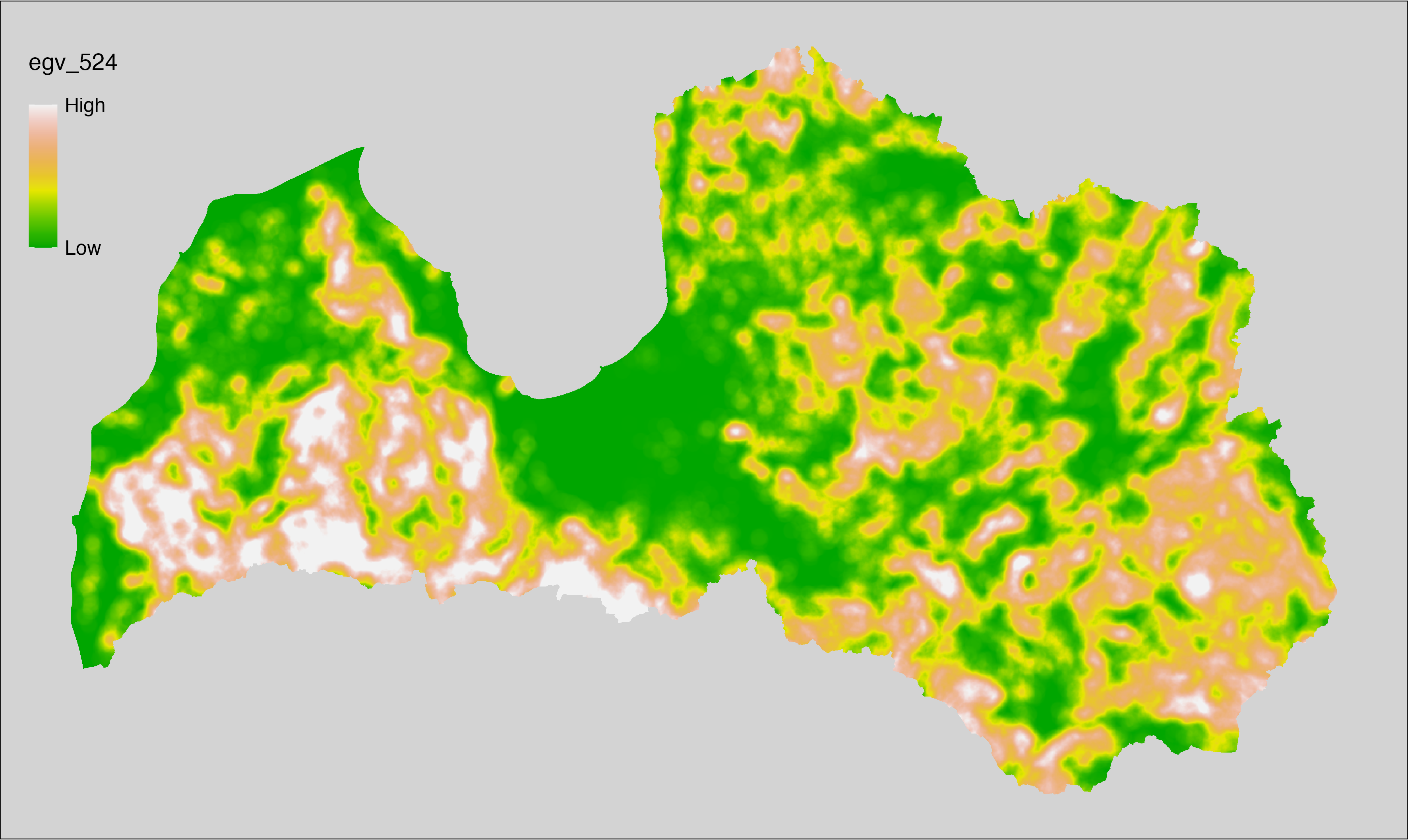
6.525 SoilTexture_Silt_r10000
filename: SoilTexture_Silt_r10000.tif
layername: egv_525
English name: Fractional cover of Silt Soils within the 10 km landscape
Latvian name: Augsnes granulometriskās klases “smilšmāls un mālsmilts” platības īpatsvars 10 km ainavā
Procedure: The cover fraction within a radius of 10000 m around the analysis grid cell is
calculated as the area-weighted sum of the analysis cells inside the
buffer, using the workflow egvtools::radius_function(). During the calculation of the landscape metric,
inverse distance weighted (power = 2) gap filling on the output is applied
to ensure no missing values at the edges. Then the layer is rewritten to set
its name. Finally, the layer is standardised by subtracting the arithmetic
mean and dividing by the root mean squared error.
Code
# libs ----
if(!require(terra)) {install.packages("terra"); require(terra)}
if(!require(egvtools)) {remotes::install_github("aavotins/egvtools"); require(egvtools)}
# EGVs radii ----
radius_function(
kvadrati_path = "./Templates/TemplateGrids/tiles/",
radii_path = "./Templates/TemplateGridPoints/tiles/",
tikls100_path = "./Templates/TemplateGrids/tikls100_sauzeme.parquet",
template_path = "./Templates/TemplateRasters/LV100m_10km.tif",
input_layers = c("./RasterGrids_100m/2024/RAW/SoilTexture_Silt_cell.tif"),
layer_prefixes = c("SoilTexture_Silt"),
output_dir = "./RasterGrids_100m/2024/RAW/",
n_workers = 5,
radii = c("r10000"),
radius_mode = "sparse",
extract_fun = "mean",
fill_missing = TRUE,
IDW_weight = 2,
future_max_size = 5 * 1024^3)
# SoilTexture_Silt_r10000.tif egv_525
slanis=rast("./RasterGrids_100m/2024/RAW/SoilTexture_Silt_r10000.tif")
names(slanis)="egv_525"
slanis2=project(slanis,template100)
writeRaster(slanis2,
"./RasterGrids_100m/2024/RAW/SoilTexture_Silt_r10000.tif",
overwrite=TRUE)
# standardisation ----
if(!require(terra)) {install.packages("terra"); require(terra)}
if(!require(tidyverse)) {install.packages("tidyverse"); require(tidyverse)}
nosaukums="SoilTexture_Silt_r10000.tif"
ielasisanas_cels=paste0("./RasterGrids_100m/2024/RAW/",nosaukums)
saglabasanas_cels=paste0("./RasterGrids_100m/2024/Scaled/",nosaukums)
slanis=rast(ielasisanas_cels)
videjais=global(slanis,fun="mean",na.rm=TRUE)
centrets=slanis-videjais[,1]
standartnovirze=terra::global(centrets,fun="rms",na.rm=TRUE)
merogots=centrets/standartnovirze[,1]
writeRaster(merogots,
filename=saglabasanas_cels,
overwrite=TRUE)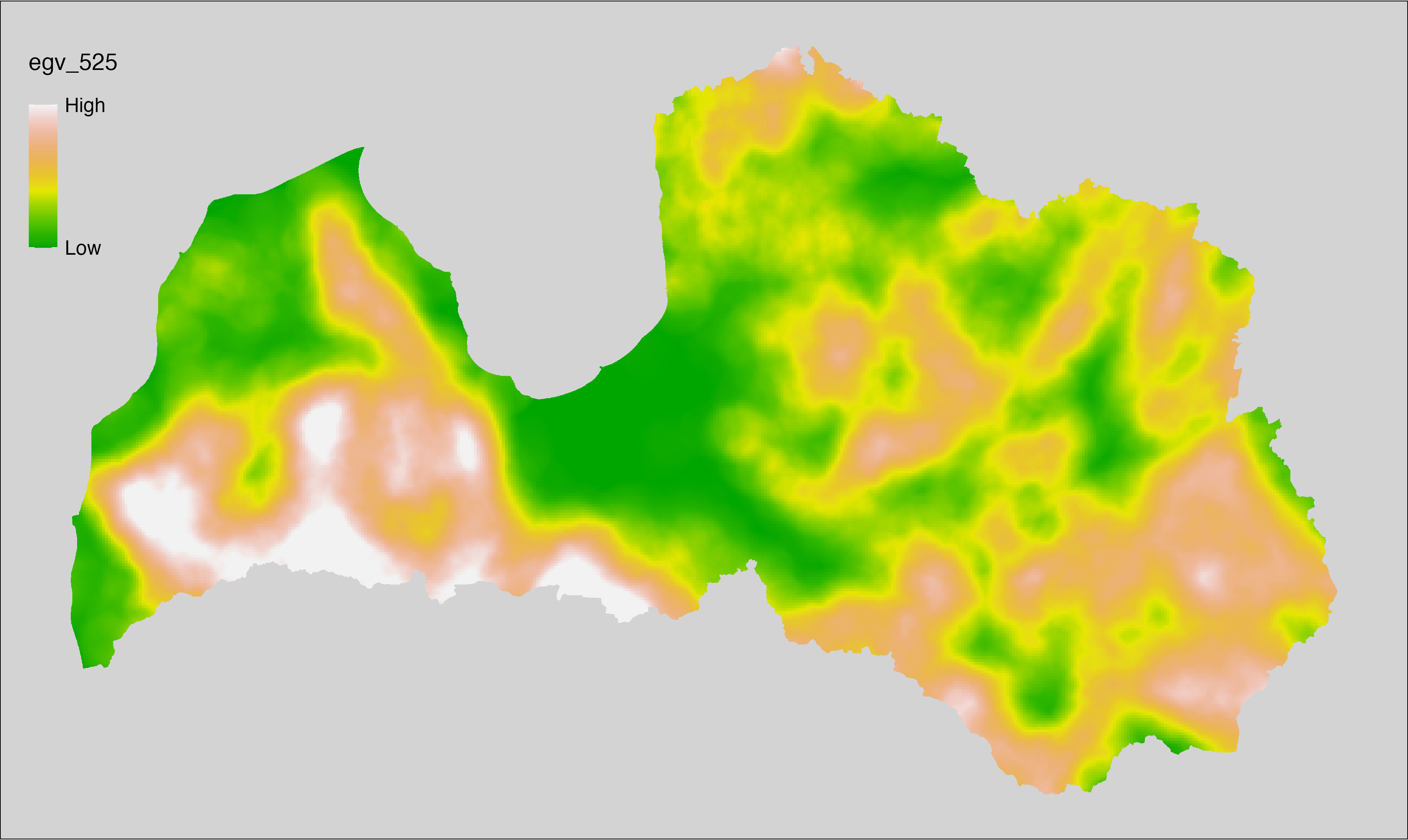
6.526 Terrain_ASL-average_cell
filename: Terrain_ASL-average_cell.tif
layername: egv_526
English name: Average value of height Above Sea Level (m) within the analysis cell (1 ha)
Latvian name: Augstums virs jūras līmeņa (m) analīzes šūnā (1 ha)
Procedure: Derived from the Digital elevation/terrain models.
Processed using the workflow egvtools::input2egv(). Inverse distance
weighted (power = 2) gap filling is implemented to protect against potential data
loss at edge cells. Finally, the layer is standardised by subtracting the
arithmetic mean and dividing by the root mean squared error.
Code
# libs ----
if(!require(terra)) {install.packages("terra"); require(terra)}
if(!require(egvtools)) {remotes::install_github("aavotins/egvtools"); require(egvtools)}
# templates ----
template100=rast("./Templates/TemplateRasters/LV100m_10km.tif")
# Terrain_ASL-average_cell.tif egv_526
input2egv(input="./Geodata/2024/DEM/mozDEM_10m.tif",
egv_template="./Templates/TemplateRasters/LV100m_10km.tif",
summary_function = "average",
missing_job = "FillOutput",
idw_weight = 2,
outlocation = "./RasterGrids_100m/2024/RAW/",
outfilename = "Terrain_ASL-average_cell.tif",
layername="egv_526",
return_visible = TRUE,
plot_final = TRUE)
# standardisation ----
if(!require(terra)) {install.packages("terra"); require(terra)}
if(!require(tidyverse)) {install.packages("tidyverse"); require(tidyverse)}
nosaukums="Terrain_ASL-average_cell.tif"
ielasisanas_cels=paste0("./RasterGrids_100m/2024/RAW/",nosaukums)
saglabasanas_cels=paste0("./RasterGrids_100m/2024/Scaled/",nosaukums)
slanis=rast(ielasisanas_cels)
videjais=global(slanis,fun="mean",na.rm=TRUE)
centrets=slanis-videjais[,1]
standartnovirze=terra::global(centrets,fun="rms",na.rm=TRUE)
merogots=centrets/standartnovirze[,1]
writeRaster(merogots,
filename=saglabasanas_cels,
overwrite=TRUE)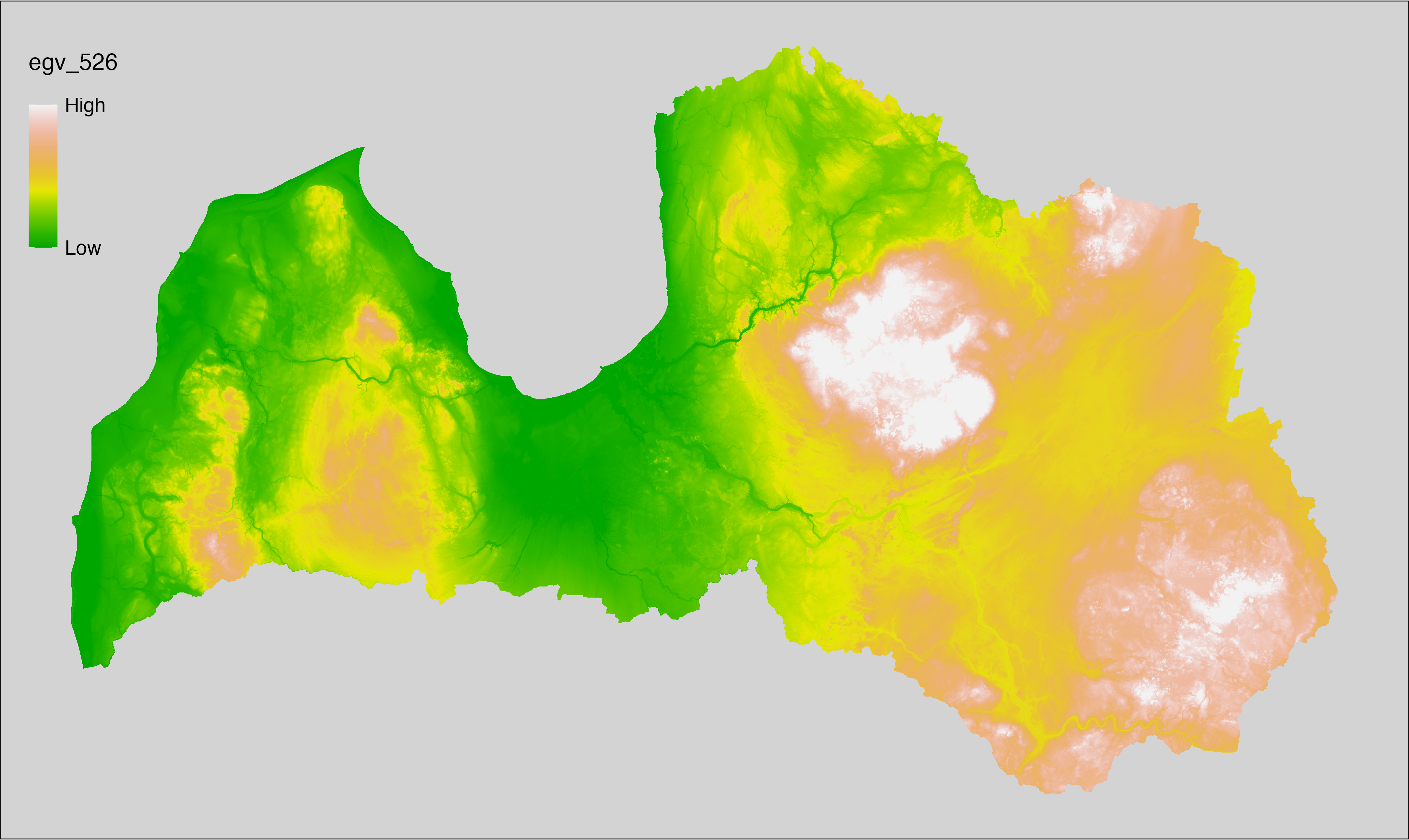
6.527 Terrain_Aspect-average_cell
filename: Terrain_Aspect-average_cell.tif
layername: egv_527
English name: Average value of Terrain Aspect (degree) within the analysis cell (1 ha)
Latvian name: Nogāzes vidējais vērsuma virziens (grādi) analīzes šūnā (1 ha)
Procedure: Derived from the Terrain products.
Processed using the workflow egvtools::input2egv(). Inverse distance
weighted (power = 2) gap filling is implemented to protect against potential data
loss at edge cells. Finally, the layer is standardised by subtracting the
arithmetic mean and dividing by the root mean squared error.
Code
# libs ----
if(!require(terra)) {install.packages("terra"); require(terra)}
if(!require(egvtools)) {remotes::install_github("aavotins/egvtools"); require(egvtools)}
# templates ----
template100=rast("./Templates/TemplateRasters/LV100m_10km.tif")
# Terrain_Aspect-average_cell.tif egv_527
input2egv(input="./RasterGrids_10m/2024/Terrain_Aspect_udeni2_10m.tif",
egv_template="./Templates/TemplateRasters/LV100m_10km.tif",
summary_function = "average",
missing_job = "FillOutput",
idw_weight = 2,
outlocation = "./RasterGrids_100m/2024/RAW/",
outfilename = "Terrain_Aspect-average_cell.tif",
layername="egv_527",
return_visible = TRUE,
plot_final = TRUE)
# standardisation ----
if(!require(terra)) {install.packages("terra"); require(terra)}
if(!require(tidyverse)) {install.packages("tidyverse"); require(tidyverse)}
nosaukums="Terrain_Aspect-average_cell.tif"
ielasisanas_cels=paste0("./RasterGrids_100m/2024/RAW/",nosaukums)
saglabasanas_cels=paste0("./RasterGrids_100m/2024/Scaled/",nosaukums)
slanis=rast(ielasisanas_cels)
videjais=global(slanis,fun="mean",na.rm=TRUE)
centrets=slanis-videjais[,1]
standartnovirze=terra::global(centrets,fun="rms",na.rm=TRUE)
merogots=centrets/standartnovirze[,1]
writeRaster(merogots,
filename=saglabasanas_cels,
overwrite=TRUE)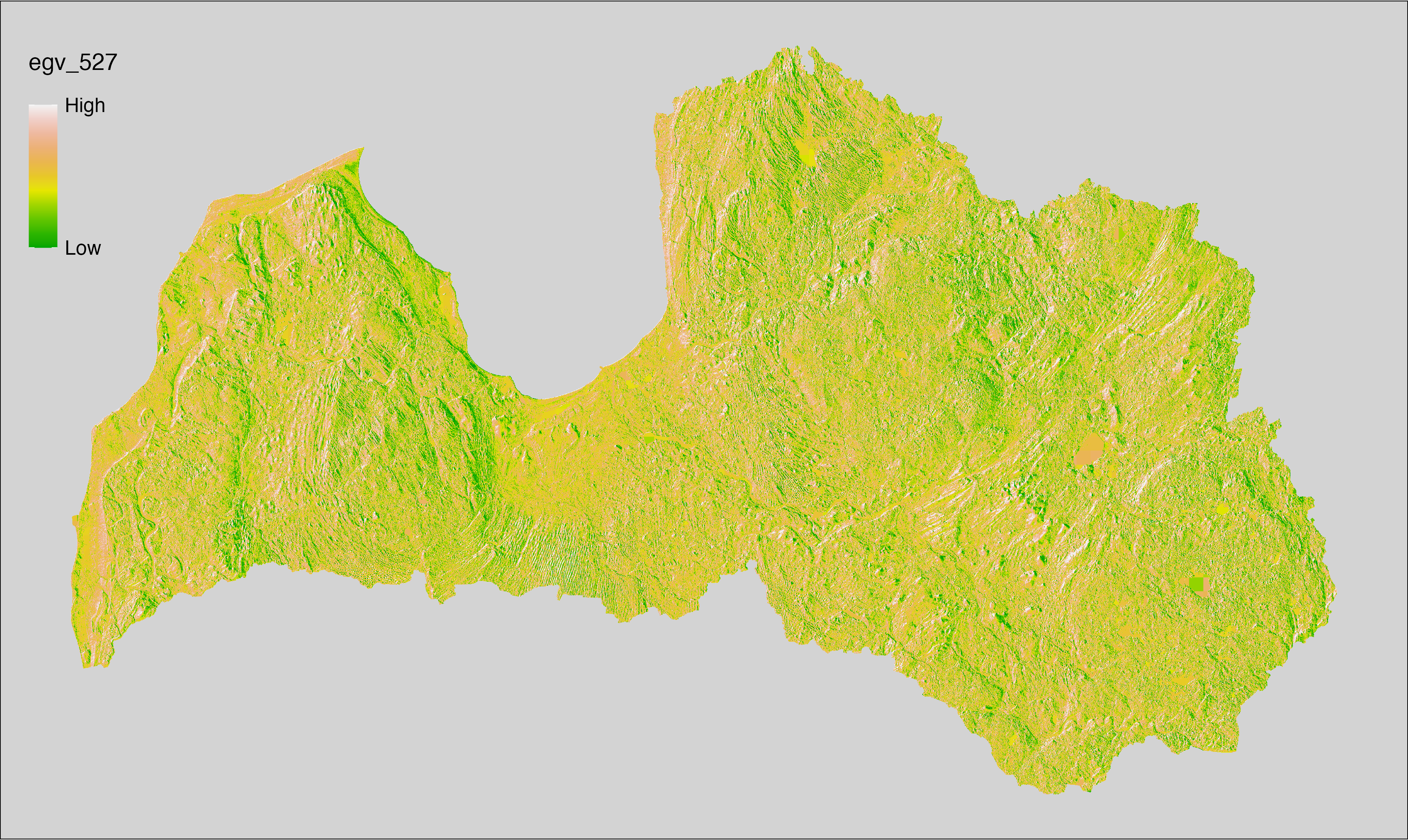
6.528 Terrain_Aspect-iqr_cell
filename: Terrain_Aspect-iqr_cell.tif
layername: egv_528
English name: Variability of Terrain Aspect (degree) within the analysis cell (1 ha)
Latvian name: Nogāzes vērsuma (grādi) variabilitāte analīzes šūnā (1 ha)
Procedure: Derived from the Terrain products. The
workflow egvtools::input2egv() is used to calculate Q1 and Q3 for every cell.
To protect against potential data loss at the edges, inverse distance
weighted (power = 2) gap filling is implemented. Next, Q1 is subtracted from Q3.
Finally, the layer is standardised by subtracting the arithmetic mean and
dividing by the root mean squared error.
Code
# libs ----
if(!require(terra)) {install.packages("terra"); require(terra)}
if(!require(egvtools)) {remotes::install_github("aavotins/egvtools"); require(egvtools)}
# templates ----
template100=rast("./Templates/TemplateRasters/LV100m_10km.tif")
# Terrain_Aspect-iqr_cell.tif egv_528
p25rez=input2egv(input="./RasterGrids_10m/2024/Terrain_Aspect_udeni2_10m.tif",
egv_template= "./Templates/TemplateRasters/LV100m_10km.tif",
summary_function = "q1",
missing_job = "FillOutput",
outlocation = "./RasterGrids_100m/2024/",
outfilename = "draza_p25.tif",
layername = "egv_528",
idw_weight = 2)
p25rez_r=rast("./RasterGrids_100m/2024/draza_p25.tif")
p75rez=input2egv(input="./RasterGrids_10m/2024/Terrain_Aspect_udeni2_10m.tif",
egv_template= "./Templates/TemplateRasters/LV100m_10km.tif",
summary_function = "q3",
missing_job = "FillOutput",
outlocation = "./RasterGrids_100m/2024/",
outfilename = "draza_p75.tif",
layername = "egv_528",
idw_weight = 2)
p75rez_r=rast("./RasterGrids_100m/2024/draza_p75.tif")
iqr_rez=p75rez_r-p25rez_r
iqr_rez
plot(iqr_rez)
writeRaster(iqr_rez,
"./RasterGrids_100m/2024/RAW/Terrain_Aspect-iqr_cell.tif",
overwrite=TRUE)
unlink("./RasterGrids_100m/2024/draza_p75.tif")
unlink("./RasterGrids_100m/2024/draza_p25.tif")
# standardisation ----
if(!require(terra)) {install.packages("terra"); require(terra)}
if(!require(tidyverse)) {install.packages("tidyverse"); require(tidyverse)}
nosaukums="Terrain_Aspect-iqr_cell.tif"
ielasisanas_cels=paste0("./RasterGrids_100m/2024/RAW/",nosaukums)
saglabasanas_cels=paste0("./RasterGrids_100m/2024/Scaled/",nosaukums)
slanis=rast(ielasisanas_cels)
videjais=global(slanis,fun="mean",na.rm=TRUE)
centrets=slanis-videjais[,1]
standartnovirze=terra::global(centrets,fun="rms",na.rm=TRUE)
merogots=centrets/standartnovirze[,1]
writeRaster(merogots,
filename=saglabasanas_cels,
overwrite=TRUE)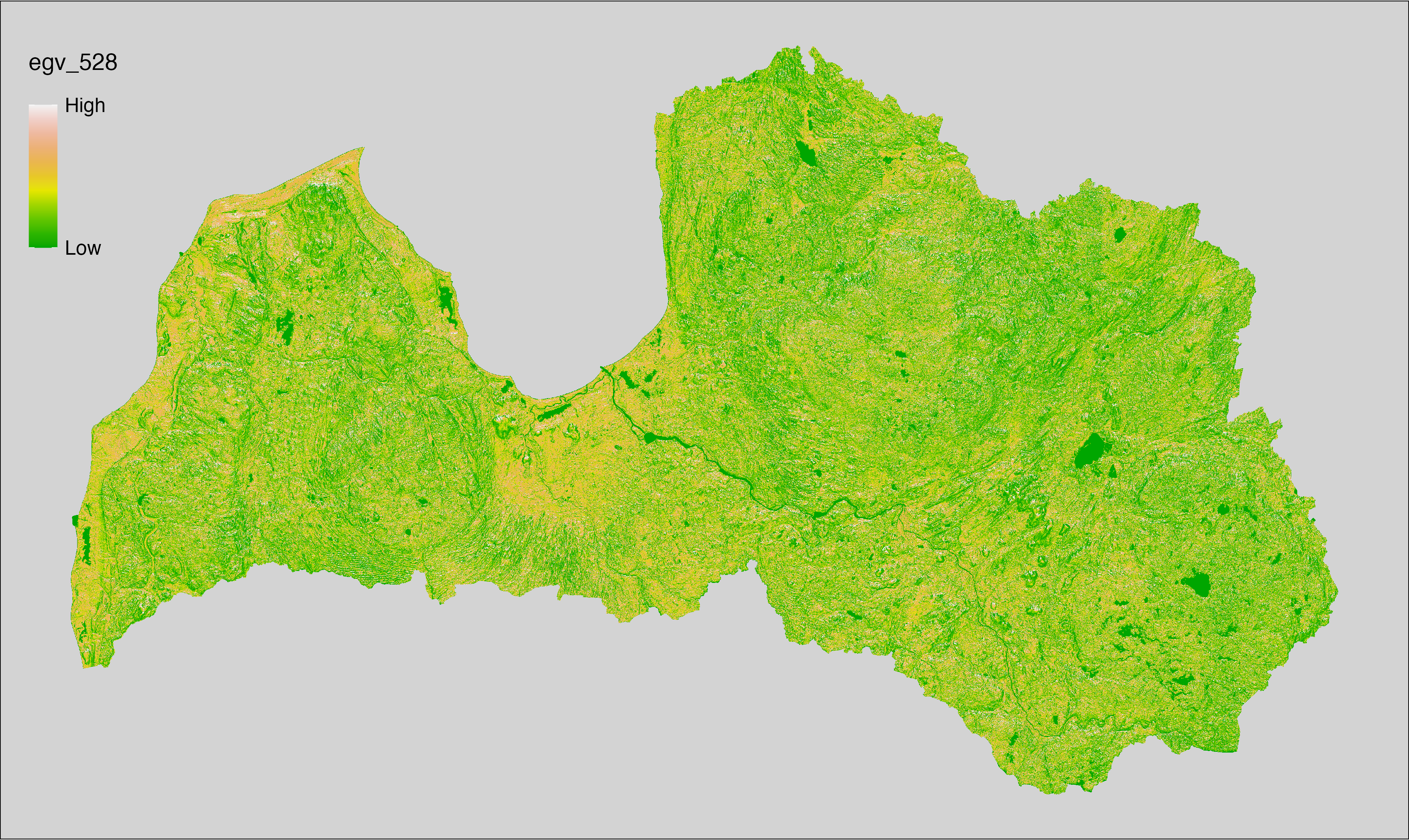
6.529 Terrain_DiS-area_cell
filename: Terrain_DiS-area_cell.tif
layername: egv_529
English name: Fractional cover of Terrain Sinks within the analysis cell (1 ha)
Latvian name: Reljefa depresiju bez virszemes noteces platības īpatsvars analīzes šūnā (1 ha)
Procedure: Derived from the Terrain products depth-in-sinks
layer, which is reclassified to a value of 1 in every cell with a positive value.
The resulting layer
is then aggregated to EGV resolution using the workflow egvtools::input2egv(), which
calculates the arithmetic mean to determine the cover fraction. During
aggregation, inverse distance weighted (power = 2) gap filling on the output is
applied to ensure no missing values at the edges. Finally, the layer is
standardised by subtracting the arithmetic mean and dividing by the root mean squared
error.
Code
# libs ----
if(!require(terra)) {install.packages("terra"); require(terra)}
if(!require(egvtools)) {remotes::install_github("aavotins/egvtools"); require(egvtools)}
# templates ----
template100=rast("./Templates/TemplateRasters/LV100m_10km.tif")
# Terrain_DiS-area_cell.tif egv_529
dis=rast("./RasterGrids_10m/2024/Terrain_DiS_udeni2_10m.tif")
dis2=ifel(dis>0,1,dis)
input2egv(input=dis2,
egv_template="./Templates/TemplateRasters/LV100m_10km.tif",
summary_function = "average",
missing_job = "FillOutput",
idw_weight = 2,
outlocation = "./RasterGrids_100m/2024/RAW/",
outfilename = "Terrain_DiS-area_cell.tif",
layername="egv_529",
return_visible = TRUE,
plot_final = TRUE)
# standardisation ----
if(!require(terra)) {install.packages("terra"); require(terra)}
if(!require(tidyverse)) {install.packages("tidyverse"); require(tidyverse)}
nosaukums="Terrain_DiS-area_cell.tif"
ielasisanas_cels=paste0("./RasterGrids_100m/2024/RAW/",nosaukums)
saglabasanas_cels=paste0("./RasterGrids_100m/2024/Scaled/",nosaukums)
slanis=rast(ielasisanas_cels)
videjais=global(slanis,fun="mean",na.rm=TRUE)
centrets=slanis-videjais[,1]
standartnovirze=terra::global(centrets,fun="rms",na.rm=TRUE)
merogots=centrets/standartnovirze[,1]
writeRaster(merogots,
filename=saglabasanas_cels,
overwrite=TRUE)
6.530 Terrain_DiS-area_r500
filename: Terrain_DiS-area_r500.tif
layername: egv_530
English name: Fractional cover of Terrain Sinks within the 0.5 km landscape
Latvian name: Reljefa depresiju bez virszemes noteces platības īpatsvars 0,5 km ainavā
Procedure: The cover fraction within a radius of 500 m around the analysis grid cell is
calculated as the area-weighted sum of the analysis cells inside the
buffer, using the workflow egvtools::radius_function(). During the calculation of the landscape metric,
inverse distance weighted (power = 2) gap filling on the output is applied
to ensure no missing values at the edges. Then the layer is rewritten to set
its name. Finally, the layer is standardised by subtracting the arithmetic
mean and dividing by the root mean squared error.
Code
# libs ----
if(!require(terra)) {install.packages("terra"); require(terra)}
if(!require(egvtools)) {remotes::install_github("aavotins/egvtools"); require(egvtools)}
# templates ----
template100=rast("./Templates/TemplateRasters/LV100m_10km.tif")
# radii
radius_function(
kvadrati_path = "./Templates/TemplateGrids/tiles/",
radii_path = "./Templates/TemplateGridPoints/tiles/",
tikls100_path = "./Templates/TemplateGrids/tikls100_sauzeme.parquet",
template_path = "./Templates/TemplateRasters/LV100m_10km.tif",
input_layers = c("./RasterGrids_100m/2024/RAW/Terrain_DiS-area_cell.tif"),
layer_prefixes = c("Terrain_DiS-area"),
output_dir = "./RasterGrids_100m/2024/RAW/",
n_workers = 5,
radii = c("r500"),
radius_mode = "sparse",
extract_fun = "mean",
fill_missing = TRUE,
IDW_weight = 2,
future_max_size = 5 * 1024^3)
# Terrain_DiS-area_r500.tif egv_530
slanis=rast("./RasterGrids_100m/2024/RAW/Terrain_DiS-area_r500.tif")
names(slanis)="egv_530"
slanis2=project(slanis,template100)
writeRaster(slanis2,
"./RasterGrids_100m/2024/RAW/Terrain_DiS-area_r500.tif",
overwrite=TRUE)
# standardisation ----
if(!require(terra)) {install.packages("terra"); require(terra)}
if(!require(tidyverse)) {install.packages("tidyverse"); require(tidyverse)}
nosaukums="Terrain_DiS-area_r500.tif"
ielasisanas_cels=paste0("./RasterGrids_100m/2024/RAW/",nosaukums)
saglabasanas_cels=paste0("./RasterGrids_100m/2024/Scaled/",nosaukums)
slanis=rast(ielasisanas_cels)
videjais=global(slanis,fun="mean",na.rm=TRUE)
centrets=slanis-videjais[,1]
standartnovirze=terra::global(centrets,fun="rms",na.rm=TRUE)
merogots=centrets/standartnovirze[,1]
writeRaster(merogots,
filename=saglabasanas_cels,
overwrite=TRUE)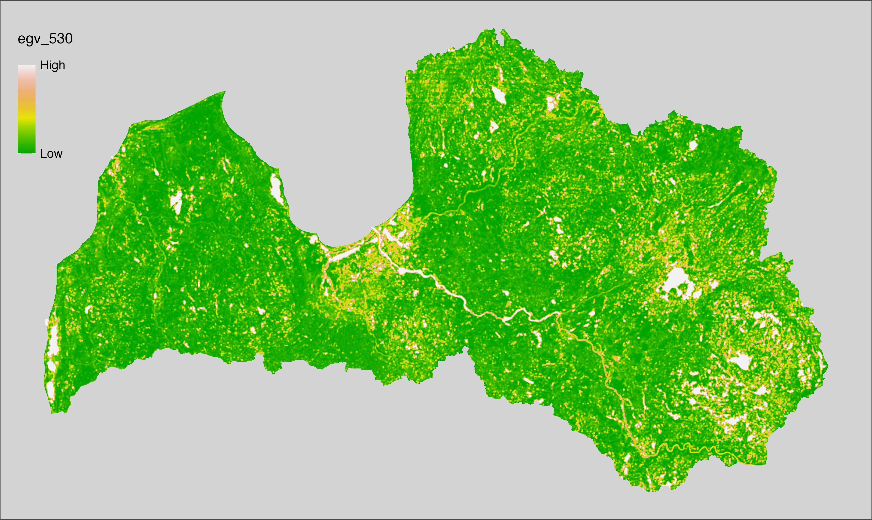
6.531 Terrain_DiS-area_r1250
filename: Terrain_DiS-area_r1250.tif
layername: egv_531
English name: Fractional cover of Terrain Sinks within the 1.25 km landscape
Latvian name: Reljefa depresiju bez virszemes noteces platības īpatsvars 1,25 km ainavā
Procedure: The cover fraction within a radius of 1250 m around the analysis grid cell is
calculated as the area-weighted sum of the analysis cells inside the
buffer, using the workflow egvtools::radius_function(). During the calculation of the landscape metric,
inverse distance weighted (power = 2) gap filling on the output is applied
to ensure no missing values at the edges. Then the layer is rewritten to set
its name. Finally, the layer is standardised by subtracting the arithmetic
mean and dividing by the root mean squared error.
Code
# libs ----
if(!require(terra)) {install.packages("terra"); require(terra)}
if(!require(egvtools)) {remotes::install_github("aavotins/egvtools"); require(egvtools)}
# templates ----
template100=rast("./Templates/TemplateRasters/LV100m_10km.tif")
# radii
radius_function(
kvadrati_path = "./Templates/TemplateGrids/tiles/",
radii_path = "./Templates/TemplateGridPoints/tiles/",
tikls100_path = "./Templates/TemplateGrids/tikls100_sauzeme.parquet",
template_path = "./Templates/TemplateRasters/LV100m_10km.tif",
input_layers = c("./RasterGrids_100m/2024/RAW/Terrain_DiS-area_cell.tif"),
layer_prefixes = c("Terrain_DiS-area"),
output_dir = "./RasterGrids_100m/2024/RAW/",
n_workers = 5,
radii = c("r1250"),
radius_mode = "sparse",
extract_fun = "mean",
fill_missing = TRUE,
IDW_weight = 2,
future_max_size = 5 * 1024^3)
# Terrain_DiS-area_r1250.tif egv_531
slanis=rast("./RasterGrids_100m/2024/RAW/Terrain_DiS-area_r1250.tif")
names(slanis)="egv_531"
slanis2=project(slanis,template100)
writeRaster(slanis2,
"./RasterGrids_100m/2024/RAW/Terrain_DiS-area_r1250.tif",
overwrite=TRUE)
# standardisation ----
if(!require(terra)) {install.packages("terra"); require(terra)}
if(!require(tidyverse)) {install.packages("tidyverse"); require(tidyverse)}
nosaukums="Terrain_DiS-area_r1250.tif"
ielasisanas_cels=paste0("./RasterGrids_100m/2024/RAW/",nosaukums)
saglabasanas_cels=paste0("./RasterGrids_100m/2024/Scaled/",nosaukums)
slanis=rast(ielasisanas_cels)
videjais=global(slanis,fun="mean",na.rm=TRUE)
centrets=slanis-videjais[,1]
standartnovirze=terra::global(centrets,fun="rms",na.rm=TRUE)
merogots=centrets/standartnovirze[,1]
writeRaster(merogots,
filename=saglabasanas_cels,
overwrite=TRUE)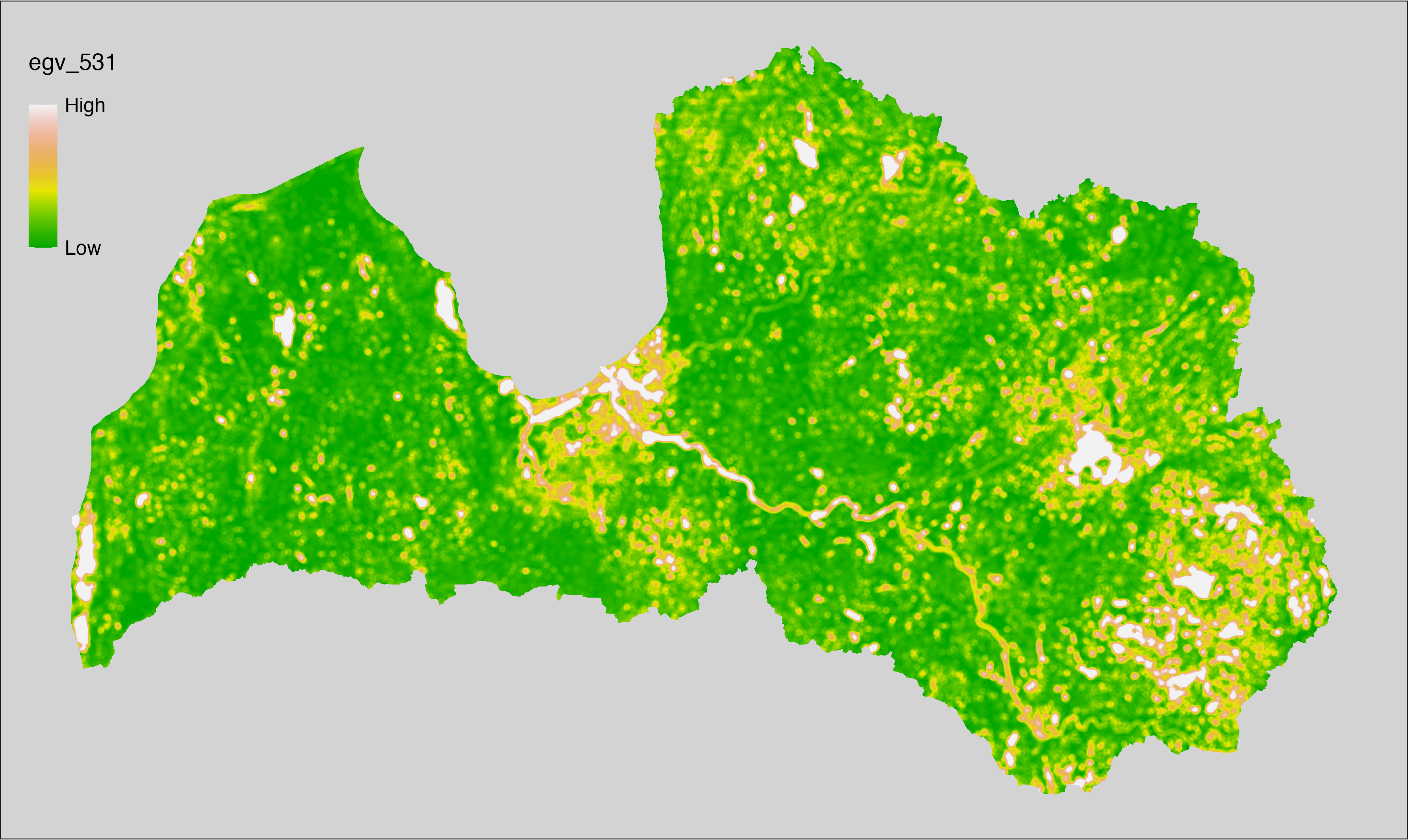
6.532 Terrain_DiS-area_r3000
filename: Terrain_DiS-area_r3000.tif
layername: egv_532
English name: Fractional cover of Terrain Sinks within the 3 km landscape
Latvian name: Reljefa depresiju bez virszemes noteces platības īpatsvars 3 km ainavā
Procedure: The cover fraction within a radius of 3000 m around the analysis grid cell is
calculated as the area-weighted sum of the analysis cells inside the
buffer, using the workflow egvtools::radius_function(). During the calculation of the landscape metric,
inverse distance weighted (power = 2) gap filling on the output is applied
to ensure no missing values at the edges. Then the layer is rewritten to set
its name. Finally, the layer is standardised by subtracting the arithmetic
mean and dividing by the root mean squared error.
Code
# libs ----
if(!require(terra)) {install.packages("terra"); require(terra)}
if(!require(egvtools)) {remotes::install_github("aavotins/egvtools"); require(egvtools)}
# templates ----
template100=rast("./Templates/TemplateRasters/LV100m_10km.tif")
# radii
radius_function(
kvadrati_path = "./Templates/TemplateGrids/tiles/",
radii_path = "./Templates/TemplateGridPoints/tiles/",
tikls100_path = "./Templates/TemplateGrids/tikls100_sauzeme.parquet",
template_path = "./Templates/TemplateRasters/LV100m_10km.tif",
input_layers = c("./RasterGrids_100m/2024/RAW/Terrain_DiS-area_cell.tif"),
layer_prefixes = c("Terrain_DiS-area"),
output_dir = "./RasterGrids_100m/2024/RAW/",
n_workers = 5,
radii = c("r3000"),
radius_mode = "sparse",
extract_fun = "mean",
fill_missing = TRUE,
IDW_weight = 2,
future_max_size = 5 * 1024^3)
# Terrain_DiS-area_r3000.tif egv_532
slanis=rast("./RasterGrids_100m/2024/RAW/Terrain_DiS-area_r3000.tif")
names(slanis)="egv_532"
slanis2=project(slanis,template100)
writeRaster(slanis2,
"./RasterGrids_100m/2024/RAW/Terrain_DiS-area_r3000.tif",
overwrite=TRUE)
# standardisation ----
if(!require(terra)) {install.packages("terra"); require(terra)}
if(!require(tidyverse)) {install.packages("tidyverse"); require(tidyverse)}
nosaukums="Terrain_DiS-area_r3000.tif"
ielasisanas_cels=paste0("./RasterGrids_100m/2024/RAW/",nosaukums)
saglabasanas_cels=paste0("./RasterGrids_100m/2024/Scaled/",nosaukums)
slanis=rast(ielasisanas_cels)
videjais=global(slanis,fun="mean",na.rm=TRUE)
centrets=slanis-videjais[,1]
standartnovirze=terra::global(centrets,fun="rms",na.rm=TRUE)
merogots=centrets/standartnovirze[,1]
writeRaster(merogots,
filename=saglabasanas_cels,
overwrite=TRUE)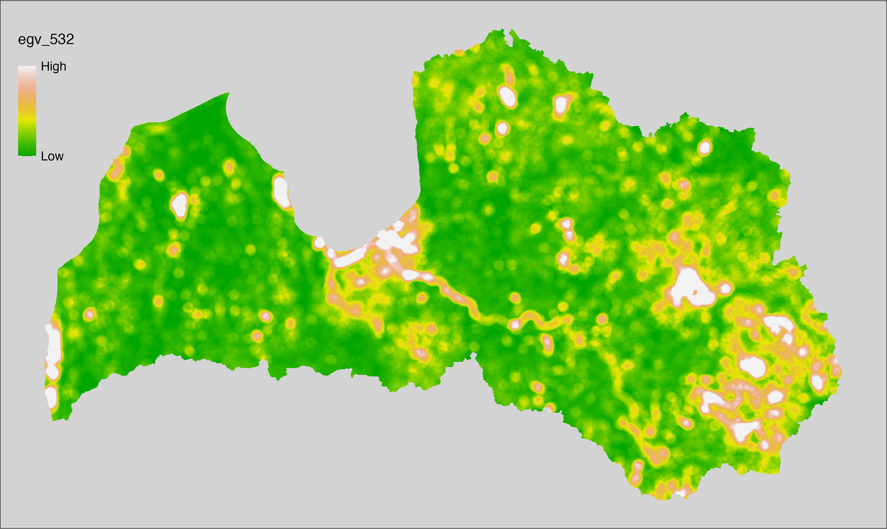
6.533 Terrain_DiS-area_r10000
filename: Terrain_DiS-area_r10000.tif
layername: egv_533
English name: Fractional cover of Terrain Sinks within the 10 km landscape
Latvian name: Reljefa depresiju bez virszemes noteces platības īpatsvars 10 km ainavā
Procedure: The cover fraction within a radius of 10000 m around the analysis grid cell is
calculated as the area-weighted sum of the analysis cells inside the
buffer, using the workflow egvtools::radius_function(). During the calculation of the landscape metric,
inverse distance weighted (power = 2) gap filling on the output is applied
to ensure no missing values at the edges. Then the layer is rewritten to set
its name. Finally, the layer is standardised by subtracting the arithmetic
mean and dividing by the root mean squared error.
Code
# libs ----
if(!require(terra)) {install.packages("terra"); require(terra)}
if(!require(egvtools)) {remotes::install_github("aavotins/egvtools"); require(egvtools)}
# templates ----
template100=rast("./Templates/TemplateRasters/LV100m_10km.tif")
# radii
radius_function(
kvadrati_path = "./Templates/TemplateGrids/tiles/",
radii_path = "./Templates/TemplateGridPoints/tiles/",
tikls100_path = "./Templates/TemplateGrids/tikls100_sauzeme.parquet",
template_path = "./Templates/TemplateRasters/LV100m_10km.tif",
input_layers = c("./RasterGrids_100m/2024/RAW/Terrain_DiS-area_cell.tif"),
layer_prefixes = c("Terrain_DiS-area"),
output_dir = "./RasterGrids_100m/2024/RAW/",
n_workers = 5,
radii = c("r10000"),
radius_mode = "sparse",
extract_fun = "mean",
fill_missing = TRUE,
IDW_weight = 2,
future_max_size = 5 * 1024^3)
# Terrain_DiS-area_r10000.tif egv_533
slanis=rast("./RasterGrids_100m/2024/RAW/Terrain_DiS-area_r10000.tif")
names(slanis)="egv_533"
slanis2=project(slanis,template100)
writeRaster(slanis2,
"./RasterGrids_100m/2024/RAW/Terrain_DiS-area_r10000.tif",
overwrite=TRUE)
# standardisation ----
if(!require(terra)) {install.packages("terra"); require(terra)}
if(!require(tidyverse)) {install.packages("tidyverse"); require(tidyverse)}
nosaukums="Terrain_DiS-area_r10000.tif"
ielasisanas_cels=paste0("./RasterGrids_100m/2024/RAW/",nosaukums)
saglabasanas_cels=paste0("./RasterGrids_100m/2024/Scaled/",nosaukums)
slanis=rast(ielasisanas_cels)
videjais=global(slanis,fun="mean",na.rm=TRUE)
centrets=slanis-videjais[,1]
standartnovirze=terra::global(centrets,fun="rms",na.rm=TRUE)
merogots=centrets/standartnovirze[,1]
writeRaster(merogots,
filename=saglabasanas_cels,
overwrite=TRUE)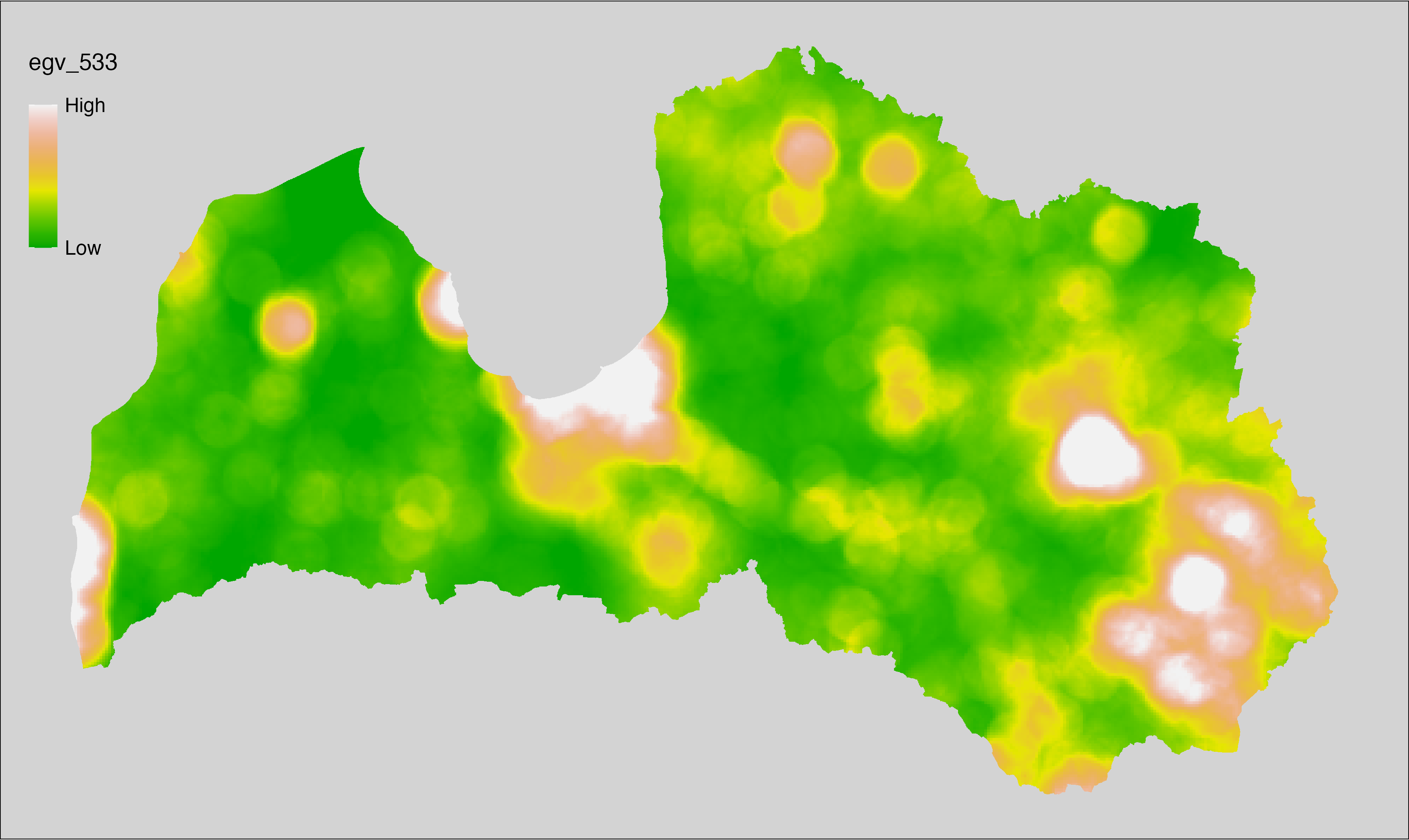
6.534 Terrain_DiS-max_cell
filename: Terrain_DiS-max_cell.tif
layername: egv_534
English name: Maximum Depth in Terrain Sink within the analysis cell (1 ha)
Latvian name: Reljefa depresiju lielākais dziļums analīzes šūnā (1 ha)
Procedure: Derived from the Terrain products.
Processed using the workflow egvtools::input2egv(). Inverse distance
weighted (power = 2) gap filling is implemented to protect against potential data
loss at edge cells. Finally, the layer is standardised by subtracting the
arithmetic mean and dividing by the root mean squared error.
Code
# libs ----
if(!require(terra)) {install.packages("terra"); require(terra)}
if(!require(egvtools)) {remotes::install_github("aavotins/egvtools"); require(egvtools)}
# templates ----
template100=rast("./Templates/TemplateRasters/LV100m_10km.tif")
# Terrain_DiS-max_cell.tif egv_534
input2egv(input="./RasterGrids_10m/2024/Terrain_DiS_udeni2_10m.tif",
egv_template="./Templates/TemplateRasters/LV100m_10km.tif",
summary_function = "max",
missing_job = "FillOutput",
idw_weight = 2,
outlocation = "./RasterGrids_100m/2024/RAW/",
outfilename = "Terrain_DiS-max_cell.tif",
layername="egv_534",
return_visible = TRUE,
plot_final = TRUE)
# standardisation ----
if(!require(terra)) {install.packages("terra"); require(terra)}
if(!require(tidyverse)) {install.packages("tidyverse"); require(tidyverse)}
nosaukums="Terrain_DiS-max_cell.tif"
ielasisanas_cels=paste0("./RasterGrids_100m/2024/RAW/",nosaukums)
saglabasanas_cels=paste0("./RasterGrids_100m/2024/Scaled/",nosaukums)
slanis=rast(ielasisanas_cels)
videjais=global(slanis,fun="mean",na.rm=TRUE)
centrets=slanis-videjais[,1]
standartnovirze=terra::global(centrets,fun="rms",na.rm=TRUE)
merogots=centrets/standartnovirze[,1]
writeRaster(merogots,
filename=saglabasanas_cels,
overwrite=TRUE)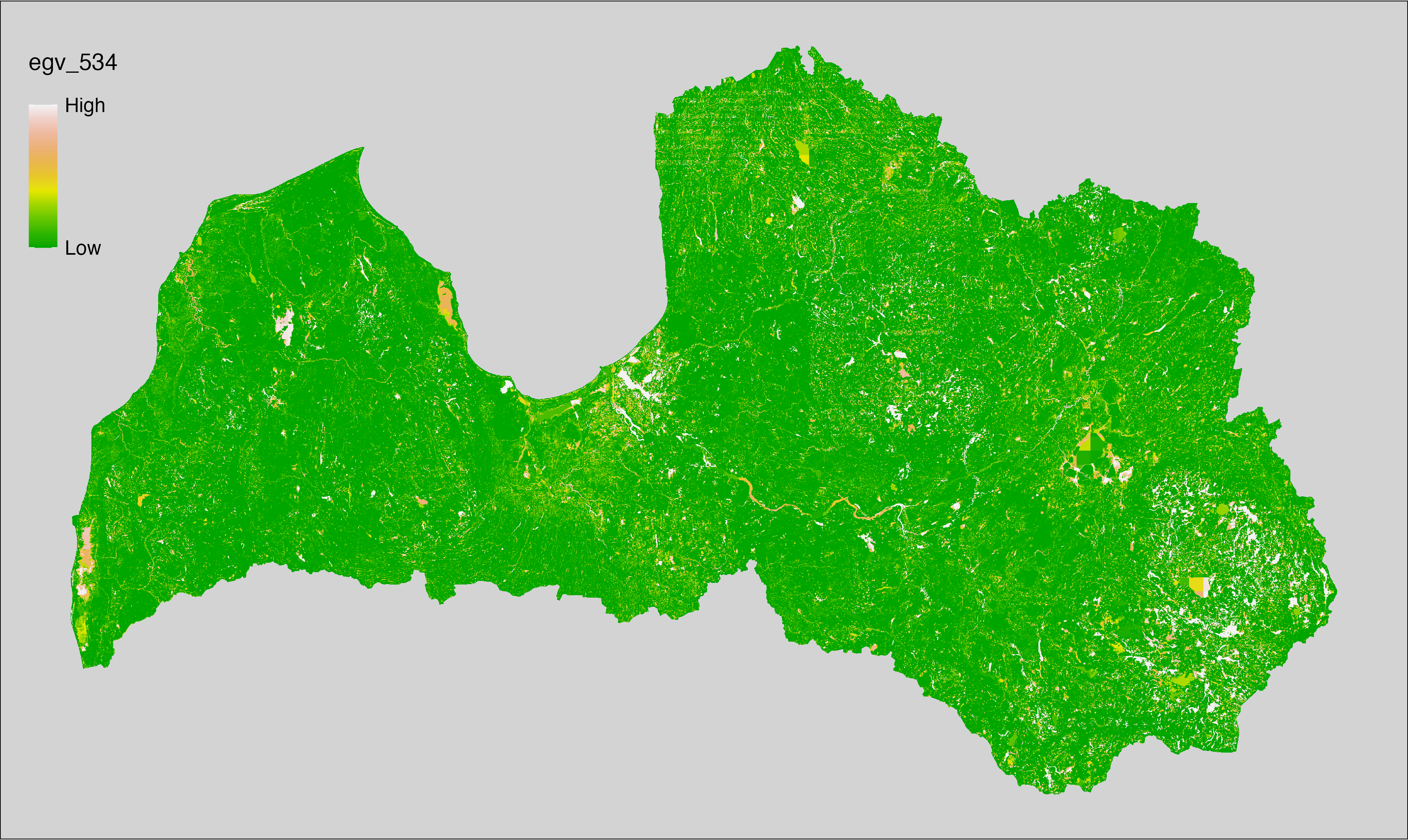
6.535 Terrain_DiS-mean_cell
filename: Terrain_DiS-mean_cell.tif
layername: egv_535
English name: Average Depth in Terrain Sink within the analysis cell (1 ha)
Latvian name: Reljefa depresiju vidējais dziļums analīzes šūnā (1 ha)
Procedure: Derived from the Terrain products.
Processed using the workflow egvtools::input2egv(). Inverse distance
weighted (power = 2) gap filling is implemented to protect against potential data
loss at edge cells. Finally, the layer is standardised by subtracting the
arithmetic mean and dividing by the root mean squared error.
Code
# libs ----
if(!require(terra)) {install.packages("terra"); require(terra)}
if(!require(egvtools)) {remotes::install_github("aavotins/egvtools"); require(egvtools)}
# templates ----
template100=rast("./Templates/TemplateRasters/LV100m_10km.tif")
# Terrain_DiS-mean_cell.tif egv_535
input2egv(input="./RasterGrids_10m/2024/Terrain_DiS_udeni2_10m.tif",
egv_template="./Templates/TemplateRasters/LV100m_10km.tif",
summary_function = "average",
missing_job = "FillOutput",
idw_weight = 2,
outlocation = "./RasterGrids_100m/2024/RAW/",
outfilename = "Terrain_DiS-mean_cell.tif",
layername="egv_535",
return_visible = TRUE,
plot_final = TRUE)
# standardisation ----
if(!require(terra)) {install.packages("terra"); require(terra)}
if(!require(tidyverse)) {install.packages("tidyverse"); require(tidyverse)}
nosaukums="Terrain_DiS-mean_cell.tif"
ielasisanas_cels=paste0("./RasterGrids_100m/2024/RAW/",nosaukums)
saglabasanas_cels=paste0("./RasterGrids_100m/2024/Scaled/",nosaukums)
slanis=rast(ielasisanas_cels)
videjais=global(slanis,fun="mean",na.rm=TRUE)
centrets=slanis-videjais[,1]
standartnovirze=terra::global(centrets,fun="rms",na.rm=TRUE)
merogots=centrets/standartnovirze[,1]
writeRaster(merogots,
filename=saglabasanas_cels,
overwrite=TRUE)
6.536 Terrain_Slope-average_cell
filename: Terrain_Slope-average_cell.tif
layername: egv_536
English name: Average value of Terrain Slope (degree) within the analysis cell (1 ha)
Latvian name: Nogāzes slīpuma (grādi) vidējā vērtība analīzes šūnā (1 ha)
Procedure: Derived from the Terrain products.
Processed using the workflow egvtools::input2egv(). Inverse distance
weighted (power = 2) gap filling is implemented to protect against potential data
loss at edge cells. Finally, the layer is standardised by subtracting the
arithmetic mean and dividing by the root mean squared error.
Code
# libs ----
if(!require(terra)) {install.packages("terra"); require(terra)}
if(!require(egvtools)) {remotes::install_github("aavotins/egvtools"); require(egvtools)}
# templates ----
template100=rast("./Templates/TemplateRasters/LV100m_10km.tif")
# Terrain_Slope-average_cell.tif egv_536
input2egv(input="./RasterGrids_10m/2024/Terrain_Slope_udeni2_10m.tif",
egv_template="./Templates/TemplateRasters/LV100m_10km.tif",
summary_function = "average",
missing_job = "FillOutput",
idw_weight = 2,
outlocation = "./RasterGrids_100m/2024/RAW/",
outfilename = "Terrain_Slope-average_cell.tif",
layername="egv_536",
return_visible = TRUE,
plot_final = TRUE)
# standardisation ----
if(!require(terra)) {install.packages("terra"); require(terra)}
if(!require(tidyverse)) {install.packages("tidyverse"); require(tidyverse)}
nosaukums="Terrain_Slope-average_cell.tif"
ielasisanas_cels=paste0("./RasterGrids_100m/2024/RAW/",nosaukums)
saglabasanas_cels=paste0("./RasterGrids_100m/2024/Scaled/",nosaukums)
slanis=rast(ielasisanas_cels)
videjais=global(slanis,fun="mean",na.rm=TRUE)
centrets=slanis-videjais[,1]
standartnovirze=terra::global(centrets,fun="rms",na.rm=TRUE)
merogots=centrets/standartnovirze[,1]
writeRaster(merogots,
filename=saglabasanas_cels,
overwrite=TRUE)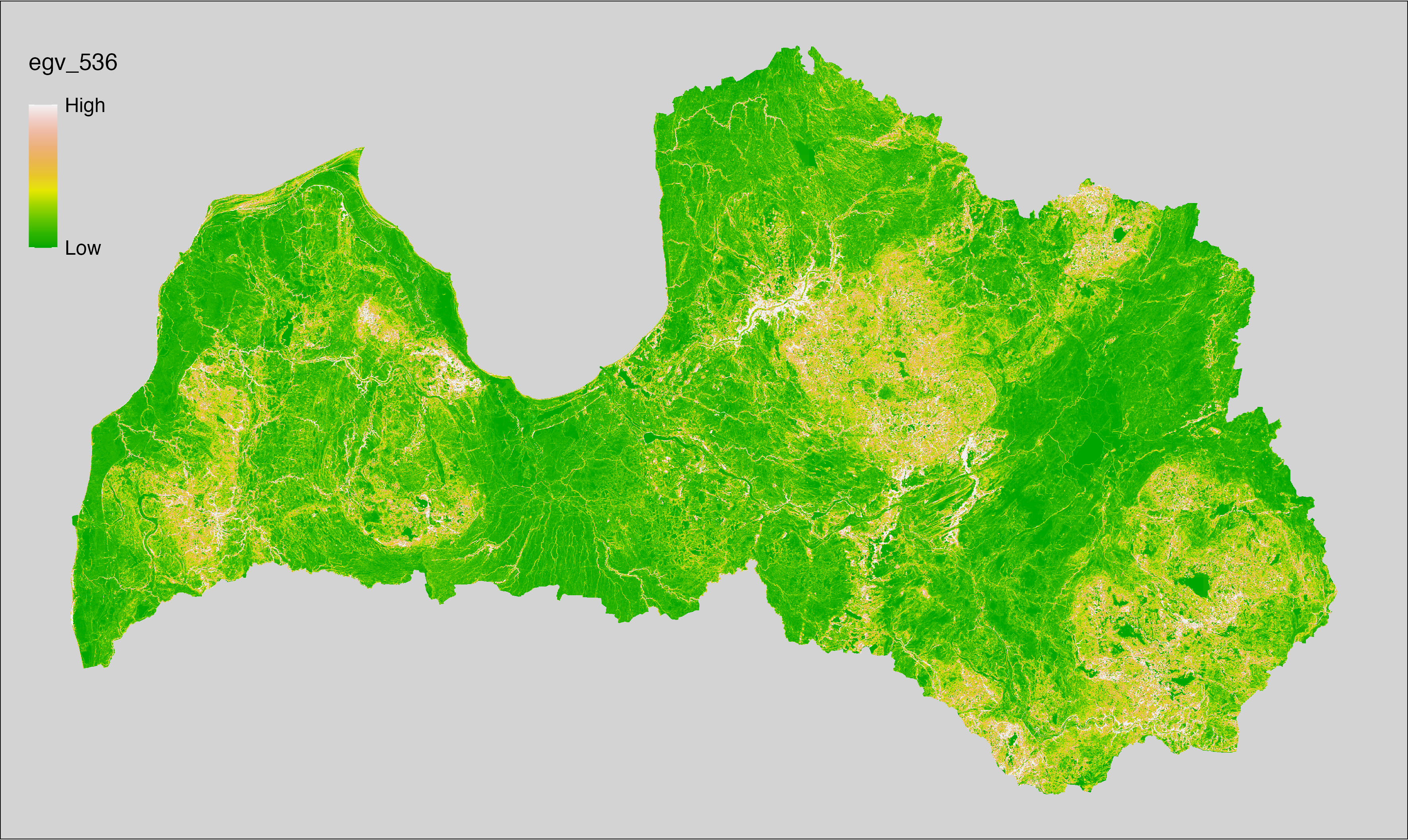
6.537 Terrain_Slope-iqr_cell
filename: Terrain_Slope-iqr_cell.tif
layername: egv_537
English name: Variability of Terrain Slope (degree) within the analysis cell (1 ha)
Latvian name: Nogāzes slīpuma (grādi) variabilitāte analīzes šūnā (1 ha)
Procedure: Derived from the Terrain products. The
workflow egvtools::input2egv() is used to calculate Q1 and Q3 for every cell.
To protect against potential data loss at the edges, inverse distance
weighted (power = 2) gap filling is implemented. Next, Q1 is subtracted from Q3.
Finally, the layer is standardised by subtracting the arithmetic mean and
dividing by the root mean squared error.
Code
# libs ----
if(!require(terra)) {install.packages("terra"); require(terra)}
if(!require(egvtools)) {remotes::install_github("aavotins/egvtools"); require(egvtools)}
# templates ----
template100=rast("./Templates/TemplateRasters/LV100m_10km.tif")
# Terrain_Slope-iqr_cell.tif egv_537
p25rez=input2egv(input="./RasterGrids_10m/2024/Terrain_Slope_udeni2_10m.tif",
egv_template= "./Templates/TemplateRasters/LV100m_10km.tif",
summary_function = "q1",
missing_job = "FillOutput",
outlocation = "./RasterGrids_100m/2024/",
outfilename = "draza_p25.tif",
layername = "egv_537",
idw_weight = 2)
p25rez_r=rast("./RasterGrids_100m/2024/draza_p25.tif")
p75rez=input2egv(input="./RasterGrids_10m/2024/Terrain_Slope_udeni2_10m.tif",
egv_template= "./Templates/TemplateRasters/LV100m_10km.tif",
summary_function = "q3",
missing_job = "FillOutput",
outlocation = "./RasterGrids_100m/2024/",
outfilename = "draza_p75.tif",
layername = "egv_537",
idw_weight = 2)
p75rez_r=rast("./RasterGrids_100m/2024/draza_p75.tif")
iqr_rez=p75rez_r-p25rez_r
iqr_rez
plot(iqr_rez)
writeRaster(iqr_rez,
"./RasterGrids_100m/2024/RAW/Terrain_Slope-iqr_cell.tif",
overwrite=TRUE)
unlink("./RasterGrids_100m/2024/draza_p75.tif")
unlink("./RasterGrids_100m/2024/draza_p25.tif")
# standardisation ----
if(!require(terra)) {install.packages("terra"); require(terra)}
if(!require(tidyverse)) {install.packages("tidyverse"); require(tidyverse)}
nosaukums="Terrain_Slope-iqr_cell.tif"
ielasisanas_cels=paste0("./RasterGrids_100m/2024/RAW/",nosaukums)
saglabasanas_cels=paste0("./RasterGrids_100m/2024/Scaled/",nosaukums)
slanis=rast(ielasisanas_cels)
videjais=global(slanis,fun="mean",na.rm=TRUE)
centrets=slanis-videjais[,1]
standartnovirze=terra::global(centrets,fun="rms",na.rm=TRUE)
merogots=centrets/standartnovirze[,1]
writeRaster(merogots,
filename=saglabasanas_cels,
overwrite=TRUE)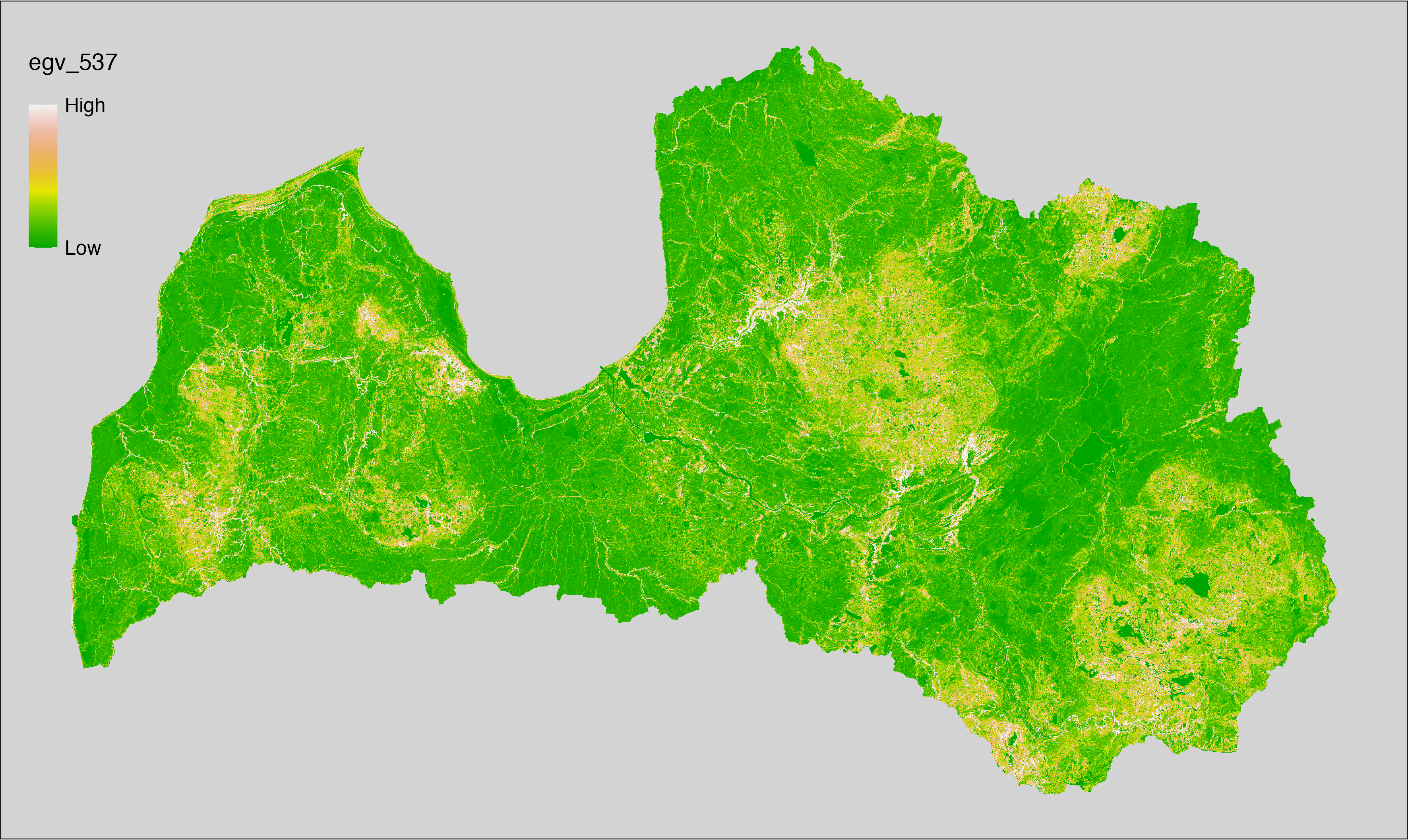
6.538 Terrain_TWI-average_cell
filename: Terrain_TWI-average_cell.tif
layername: egv_538
English name: Average value of Topographic Wetness Index (TWI) within the analysis cell (1 ha)
Latvian name: Topogrāfiskā mitruma indeksa (TWI) vidējā vērtība analīzes šūnā (1 ha)
Procedure: Derived from the Terrain products.
Processed using the workflow egvtools::input2egv(). Inverse distance
weighted (power = 2) gap filling is implemented to protect against potential data
loss at edge cells. Finally, the layer is standardised by subtracting the
arithmetic mean and dividing by the root mean squared error.
Code
# libs ----
if(!require(terra)) {install.packages("terra"); require(terra)}
if(!require(egvtools)) {remotes::install_github("aavotins/egvtools"); require(egvtools)}
# templates ----
template100=rast("./Templates/TemplateRasters/LV100m_10km.tif")
# Terrain_TWI-average_cell.tif egv_538
input2egv(input="./RasterGrids_10m/2024/Terrain_TWI_udeni2_10m.tif",
egv_template="./Templates/TemplateRasters/LV100m_10km.tif",
summary_function = "average",
missing_job = "FillOutput",
idw_weight = 2,
outlocation = "./RasterGrids_100m/2024/RAW/",
outfilename = "Terrain_TWI-average_cell.tif",
layername="egv_538",
return_visible = TRUE,
plot_final = TRUE)
# standardisation ----
if(!require(terra)) {install.packages("terra"); require(terra)}
if(!require(tidyverse)) {install.packages("tidyverse"); require(tidyverse)}
nosaukums="Terrain_TWI-average_cell.tif"
ielasisanas_cels=paste0("./RasterGrids_100m/2024/RAW/",nosaukums)
saglabasanas_cels=paste0("./RasterGrids_100m/2024/Scaled/",nosaukums)
slanis=rast(ielasisanas_cels)
videjais=global(slanis,fun="mean",na.rm=TRUE)
centrets=slanis-videjais[,1]
standartnovirze=terra::global(centrets,fun="rms",na.rm=TRUE)
merogots=centrets/standartnovirze[,1]
writeRaster(merogots,
filename=saglabasanas_cels,
overwrite=TRUE)